Identifying meteorological influences on marine low-cloud mesoscale morphology using satellite classifications
←
→
Page content transcription
If your browser does not render page correctly, please read the page content below
Atmos. Chem. Phys., 21, 9629–9642, 2021
https://doi.org/10.5194/acp-21-9629-2021
© Author(s) 2021. This work is distributed under
the Creative Commons Attribution 4.0 License.

Identifying meteorological influences on marine low-cloud
mesoscale morphology using satellite classifications
Johannes Mohrmann1 , Robert Wood1 , Tianle Yuan2,3 , Hua Song4 , Ryan Eastman1 , and Lazaros Oreopoulos2
1 Department  of Atmospheric Sciences, University of Washington, Seattle, WA, USA
2 Earth Science Division, NASA Goddard Space Flight Center, Goddard, MD, USA
3 Joint Center for Earth Systems Technology, University of Maryland, Baltimore County, Baltimore, MD, USA
4 Science Systems and Application, Inc., Lanham, MD, USA

Correspondence: Johannes Mohrmann (jkcm@uw.edu)

Received: 7 October 2020 – Discussion started: 3 November 2020
Revised: 9 April 2021 – Accepted: 29 April 2021 – Published: 28 June 2021

Abstract. Marine low-cloud mesoscale morphology in the            1   Introduction
southeastern Pacific Ocean is analyzed using a large dataset
of classifications spanning 3 years generated by machine
learning methods. Meteorological variables and cloud prop-        Marine low clouds are radiatively important, with a strong
erties are composited by the mesoscale cloud type of the clas-    cooling effect on the planet. They also display a wide range
sification, showing distinct meteorological regimes of marine     of morphologies, which have differing radiative properties
low-cloud organization from the tropics to the midlatitudes.      (Chen et al., 2000). Classically, ship-based observations have
The presentation of mesoscale cellular convection, with re-       classified marine low clouds using the familiar World Meteo-
spect to geographic distribution, boundary layer structure,       rological Organization (WMO) cloud types such as stratocu-
and large-scale environmental conditions, agrees with prior       mulus (Sc), cumulus (Cu), etc. (e.g., Warren et al., 1988).
knowledge. Two tropical and subtropical cumuliform bound-         However, clouds also form larger mesoscale, morphologi-
ary layer regimes, suppressed cumulus and clustered cumu-         cally distinct organizations that would not be apparent from
lus, are studied in detail. The patterns in precipitation, cir-   the limited perspective of a surface-based observer. These
culation, column water vapor, and cloudiness are consistent       mesoscale cloud patterns are of particular interest for sev-
with the representation of marine shallow mesoscale convec-       eral reasons. First, they have been shown to represent dif-
tive self-aggregation by large eddy simulations of the bound-     ferent underlying marine boundary layer (MBL) regimes
ary layer. Although they occur under similar large-scale con-     (e.g., Wood and Hartmann, 2006; hereafter WH06), namely
ditions, the suppressed and clustered low-cloud types are         the influence of an additional environmental MBL property
found to be well separated by variables associated with low-      that covaries with cloud morphology. Second, prior work has
level mesoscale circulation, with surface wind divergence be-     shown that the mesoscale organization regulates the relation-
ing the clearest discriminator between them, regardless of        ship between albedo and cloud fraction (CF; McCoy et al.,
whether reanalysis or satellite observations are used. Clus-      2017). Third, larger mesoscale patterns are clearly visible
tered regimes are associated with surface convergence, while      from current-generation satellite imagers, allowing for their
suppressed regimes are associated with surface divergence.        classification using computer image recognition and subse-
                                                                  quent generation of a potentially informative MBL cloud
                                                                  dataset on a near-global and highly temporally resolved scale
                                                                  for studying these clouds and their drivers.
                                                                     In the midlatitude storm tracks and eastern ocean subtropi-
                                                                  cal Sc decks, stratiform low-cloud types dominate (Hartmann
                                                                  et al., 1992). These high-cloud-fraction cloud types are par-
                                                                  ticularly effective coolers, and as a result their organization

Published by Copernicus Publications on behalf of the European Geosciences Union.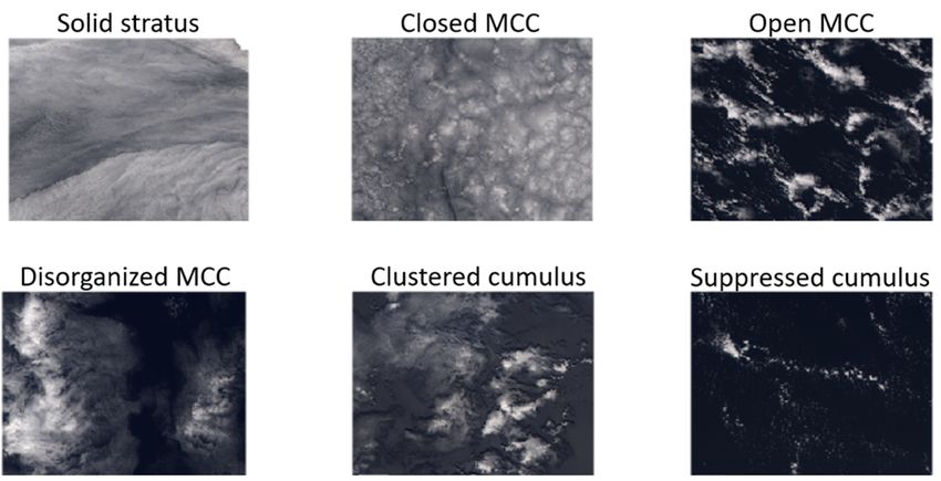
9630               J. Mohrmann et al.: Identifying meteorological influences on marine low-cloud mesoscale morphology

                                                                      conceptual model and suggested that further observational
                                                                      validation is warranted.
                                                                         When classifying stratocumulus and cumulus clouds, a
                                                                      common form of mesoscale variability is mesoscale cellu-
                                                                      lar convection (MCC) (Agee, 1987). This can take the form
                                                                      of open-cellular or closed-cellular MCC. WH06 used a neu-
                                                                      ral network to classify low-cloud scenes from satellite obser-
                                                                      vations over the eastern subtropical Pacific Ocean into four
                                                                      categories, based on MCC type or absence thereof: open,
                                                                      closed, and cellular but disorganized MCCs and no MCC
                                                                      present. The utility of these classification-based approaches
                                                                      is evident in their ability to show the controls on cloud mor-
                                                                      phology in cold air outbreaks (McCoy et al., 2017), charac-
Figure 1. Difference in relative frequency of occurrence of cumulus   terize properties and occurrences of the underlying regimes
and stratocumulus cloud types per Hahn et al. (2001) definitions      (Muhlbauer et al., 2014), or discern whether mesoscale mor-
from ship-based observations. Red areas highlight Cu-dominated        phology is more strongly driven by internal mechanisms or
MBLs, while blue regions have more Sc cloud.                          by large-scale meteorology (WH06). However, a limitation
                                                                      of the WH06 classification scheme is its inability to discrimi-
                                                                      nate between cloud morphologies over the warmer regions of
and structure have been the subject of extensive investigation        the tropical trades, where MCC is less dominant. Addition-
(Agee, 1987; Muhlbauer et al., 2014). In lower latitudes and          ally, the power-spectra- and Fourier-transform-based feature
away from the eastern subtropical ocean basins, Sc clouds             vectors used for classification were very sensitive to the pres-
are rarer, and instead we often find boundary layers (BLs)            ence of high cloud, necessitating the strict exclusion of many
dominated by cumuliform cloud types, sometimes clustering             otherwise visually identifiable scenes. More recent investi-
into large convectively active regions and some other times           gations of low-latitude marine low-cloud mesoscale variabil-
in relatively isolated smaller Cu. Figure 1, adapted from an          ity, agnostic to previously identified forms of organization,
observation-based climatic cloud atlas (Hahn and Warren,              have been successful in identifying distinct morphological
2007), shows the difference between the frequency of oc-              regimes, using machine learning to classify a large dataset of
currence of Cu clouds and that of Sc clouds; the commonly             cloud images (Stevens et al., 2020).
occurring “Cu-under-Sc” case is classified as Sc for consis-             In this work we continue the exploration of marine low-
tency with the view from above (Hahn et al., 2001). Red val-          cloud morphology drivers and characteristics with the new
ues indicate more Cu and show that boundary layer clouds              classification scheme introduced by Yuan et al. (2020) that
over the ocean between 30◦ N and S are more often cumuli-             expanded on WH06. The new scheme focuses on discrim-
form. Although the average cloud radiative effect (CRE) of            ination between different cumulus-dominated cloud types,
these clouds is lower, their ubiquity combined with a high            particularly in the tropical trade wind regions. The machine
mesoscale variability in cloud fraction makes them an im-             learning approach adopted to create this new dataset uses
portant target of study.                                              convolutional neural networks (CNNs) to permit the inclu-
   Cumuliform MBLs have been observed to contain                      sion of some scenes with thin or small amounts of high cloud.
mesoscale aggregates of shallow convection in a number                Two cumuliform low-cloud morphological types were added,
of different forms (LeMone and Meitin, 1984; Nicholls                 clustered convection and suppressed convection, to capture
and Young, 2007). Bretherton and Blossey (2017) (here-                more cloud morphological variability in the tropics and sub-
after BB17) demonstrated how mesoscale aggregation of                 tropics. Following a brief description of the new classifica-
warm shallow Cu presents in large eddy simulation (LES).              tion scheme and observational datasets (Sect. 2), we present
In their conceptual model, the shallow convective self-               the physical characteristics of the resulting cloud types in
aggregation is driven by convection–circulation–humidity              Sect. 3. Specifically, we validate in that section whether the
feedbacks. These result in cloudy regions of aggregated con-          presentation of the two cumuliform cloud types is consistent
vection with a positive mesoscale column water vapor and              with the model for mesoscale aggregation of shallow cumu-
moisture anomaly as well as a strong low-level circulation            lus convection described by BB17. We conclude with a dis-
with lower-boundary-layer convergence, acting to further              cussion of the importance of these results (Sect. 4).
concentrate moisture into the moist columns. The difference
between this and the conceptual model for deep-convective
self-aggregation (e.g., Emanuel et al., 2014) is that the lat-        2   Datasets and methods
ter relies on radiative feedbacks, which are not necessary to
produce shallow mesoscale aggregation. BB17 demonstrated              We mainly perform composite analysis of various observa-
that the presentation of shallow aggregation agrees with this         tional and model datasets by morphological cloud type. We

Atmos. Chem. Phys., 21, 9629–9642, 2021                                                 https://doi.org/10.5194/acp-21-9629-2021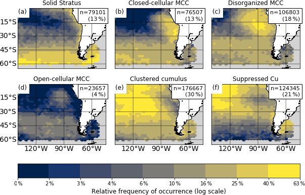
J. Mohrmann et al.: Identifying meteorological influences on marine low-cloud mesoscale morphology 9631
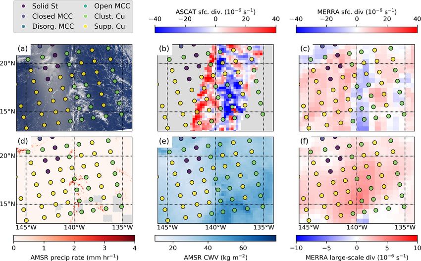
Figure 2. Typical examples of scenes belonging to each of our classification categories. Image scale is roughly 100 km across. Images are
captured using NASA Worldview.
first describe the cloud type classifications, then the datasets two types is that disorganized MCC represents a regime with
used, and finally the compositing methodology. cellular convection at some characteristic scale, though not
organized clearly into open- or closed-cell regimes, while
2.1 Cloud type classifications clustered Cu represents aggregated convection at a variety
of scales within a scene. When distinguishing between these
The classification dataset used is derived from imagery by two types during manual labeling, scene large-scale context
the Moderate-Resolution Imaging Spectrometer (MODIS), proved helpful.
aboard the Aqua satellite. MODIS RGB visible imagery of For this paper, most analysis is based on 3 years of
128 km × 128 km (approximately 1◦ × 1◦ ) cloudy scenes, fil- CNN classifications from the southeast Pacific (SEP) re-
tered to remove scenes with > 10 % coverage of high cloud, gion, (65◦ S–Equator, 140–40◦ W) which includes much of
low cloud < 5 %, and viewing angles > 45◦ , is manually the Southern Ocean and a small portion of the southwest
classified as being comprised mostly of stratus cloud, closed- Atlantic, as well as classifications from summer 2015 in
cellular marine cellular convective Sc (closed MCC), open- the northeast Pacific (NEP) region (Equator–60◦ N, 180–
cellular Sc (open MCC), disorganized-cellular stratocumulus 100◦ W) for co-location with aircraft data (see Sect. 3.5 be-
(disorganized MCC), clustered cumulus, or suppressed cu- low). The resulting tabular dataset contains location, time,
mulus. These categories were chosen by examining the mor- and cloud scene classification as well as MODIS low-
phological climatologies in Muhlbauer et al. (2014), studying cloud fraction derived from the MODIS cloud product
regions where there was little variability in morphology cat- cloud top heights (MYD06; Platnick et al., 2017). Approx-
egory (primarily the tropics, where disorganized MCC domi- imately 750 000 scenes were available for the SEP (averag-
nated), and identifying additional commonly occurring cloud ing approximately 65 classifications per MODIS granule and
morphologies. These (clustered and suppressed Cu) were 11 granules per day), while the NEP dataset is smaller, with
then added to the pre-existing cloud categories, along with ∼ 35 000 scenes. Relative distributions, normalized for each
a homogeneous stratiform category initially used in Wood location, for the various cloud scene types are provided in
and Hartmann (2006). Examples of these types can be found Fig. 3. Due to geographical differences in cloud cover and
in Fig. 2. satellite sampling, the number of viable scenes is not dis-
The scenes were then used to train a convolutional neu- tributed evenly over the regions of interest, with approxi-
ral network (CNN) using as input the image of scene visible mately 5 times as many scenes in the subtropical Sc regions
reflectance. A full description of the machine learning train- as in the midlatitudes.
ing and model evaluation can be found in Yuan et al. (2020).
These authors found that average model precision evaluated 2.2 Satellite-derived ancillary data
on a test set was approximately 93 % across all categories.
Open MCC had the lowest precision, most likely because Surface wind divergence is derived from the Advanced
it was the lowest-frequency category. The largest source of SCATterometer (ASCAT) aboard MetOp-A, specifically the
model confusion was between disorganized MCC and clus- 0.25◦ gridded wind vectors (Ricciardulli and Wentz, 2016).
tered Cu, which is unsurprising given the similar appearance For each classified scene, the 1◦ × 1◦ co-located calcu-
of these categories. The primary difference between these lated ASCAT divergence values are extracted and aver-
https://doi.org/10.5194/acp-21-9629-2021 Atmos. Chem. Phys., 21, 9629–9642, 2021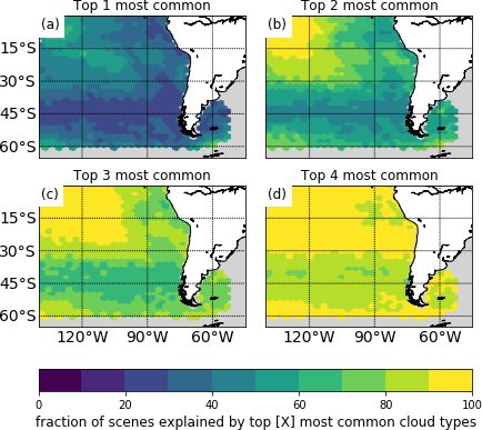
9632               J. Mohrmann et al.: Identifying meteorological influences on marine low-cloud mesoscale morphology

Figure 3. Relative frequency of occurrence of each cloud type on a logarithmic scale. In the upper right corner of each panel, the total number
of classifications over 3 years (2014–2016) as well as the total fraction of scenes of each type is shown. Gray areas are where fewer than
200 scenes are sampled.

aged. Since the ASCAT swath width is much narrower than                   longwave (LW) and shortwave (SW) fluxes (Doelling et al.,
that of MODIS (even when filtering out high-viewing-angle                 2013). These are also spatiotemporally co-located with the
scenes), many classified scenes (approximately 45 %) can-                 classified cloud scenes and used to calculate the LW, SW, and
not be paired with wind data. Additionally, the overpass                  total cloud radiative effect (CRE) for each classified scene
time of MetOp-A (∼ 09:30 LT – local time) does not co-                    via clear- and all-sky upward fluxes F :
incide with Aqua (∼ 13:30 LT) so that any significant diur-
nal cycle in wind divergence could influence results. While               CRELW = FLW,clear − FLW,all
this is a source of noise and a point of potential improve-               CRESW = FSW,clear − FSW,all
ment for future work, the diurnal amplitude in surface di-                CREtot = CRELW + CRESW .                                         (1)
vergence is likely much smaller than that of mesoscale varia-
tions (Wood et al., 2009), making the likelihood of significant           2.3   Reanalysis data
biases small. This is confirmed by repeating the divergence
analysis with the temporally better-matched reanalysis wind               For the purpose of analyzing large-scale meteorology as
data (see below), which yields similar results.                           well as comparing to satellite observations, we added data
   Column water vapor (CWV) is provided by the Ad-                        from the Modern-Era Retrospective analysis for Research
vanced Microwave Sounding Radiometer (AMSR-2) aboard                      and Application, Version 2 (MERRA-2; Gelaro et al., 2017),
the Global Change Observation Mission (GCOM-W1) satel-                    to our analysis. The data used have a 3-hourly resolution,
lite in the form of a 0.25◦ gridded daily product (Wentz et al.,          and we selected the time nearest to the MODIS-Aqua over-
2014). Being on the A-Train as Aqua, GCOM-W1 overpass                     pass. In addition to available variables (sea surface temper-
times are nearly simultaneous with those of MODIS.                        ature, near-surface winds), we derived the estimated inver-
   Rain rates come from a precipitation dataset based on                  sion strength (EIS) following Wood and Bretherton (2006),
AMSR-2 89 GHz brightness temperatures and CloudSat ob-                    a surface divergence estimated from the 10 m winds, and a
servations (Eastman et al., 2019). This particular dataset has            large-scale divergence D estimate from the 700 hPa heights
the advantage of being calibrated specifically for warm rain              and vertical motion from
from shallow marine clouds, with greater sensitivity to light                    w700
rain than other passive microwave rain products (Eastman et               D700 =
                                                                                 z700
al., 2019).                                                                        ω700
   To assess the radiative impacts of our cloud types, we also            w700 ≈ −        .                                                (2)
                                                                                   ρ700 g
analyze data from the Clouds and the Earth’s Radiant Energy
System (CERES), specifically SYN1deg hourly data, provid-                 Note that this large-scale divergence is not the horizontal
ing 1◦ , top-of-atmosphere (TOA), all-sky and clear-sky, and              divergence at 700 hPa but rather the mean divergence from

Atmos. Chem. Phys., 21, 9629–9642, 2021                                                       https://doi.org/10.5194/acp-21-9629-2021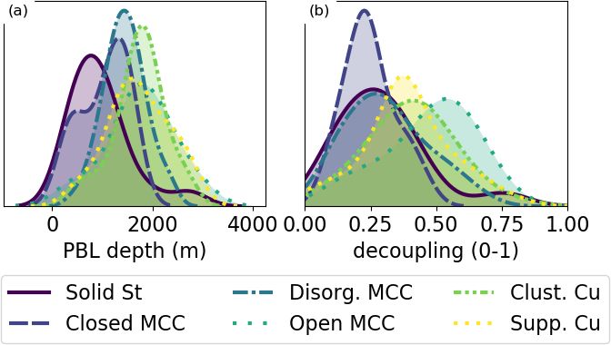
J. Mohrmann et al.: Identifying meteorological influences on marine low-cloud mesoscale morphology                          9633

the surface to the 700 hPa level; this follows from the mass      else to control for every other variable by stratifying the data
continuity equation by considering a column of air from the       in many dimensions. The approach we adopted to identify
surface (where vertical motion is 0) to 700 hPa. Note that        the extent to which differences in potential driver variables
the terms large-scale divergence and 700 hPa subsidence are       reflect short-lived anomalies compared to geographic sam-
used interchangeably throughout; divergence is plotted in-        pling bias was to calculate seasonal climatologies for each
stead of subsidence to allow for a more straightforward com-      gridded dataset and then extract for each scene the climato-
parison with surface divergence. As surface pressure varies       logical value of that field at that location. These were also
with time, the second equality is only approximate.               composited by scene cloud type and compared to the com-
   For all of the above variables (from either reanalysis or      posite of instantaneous values. This analysis is similar to the
satellite) and for each MODIS scene for which we have a           mesoscale vs. synoptic mean comparison described in the
classification, we extract the variable in a 1◦ × 1◦ box cen-     previous section but in this case using temporal deviations
tered on the cloud scene to calculate a mesoscale average         from local climatology. Figure 5a shows all three averages
value and use the mean over a 10◦ × 10◦ box for the synop-        in the same panel for direct comparison. The black circles
tic mean value. These can then be used together to calculate      represent the mesoscale (i.e., 1◦ × 1◦ average) sea surface
a mesoscale perturbation, which is simply the difference be-      temperature (SST) at that location and time, averaged over
tween the 1◦ × 1◦ and 10◦ × 10◦ averages. We also calculate       all classifications; the black diamonds are the same but aver-
a climatological 1◦ × 1◦ average by seasonal averaging.           aged over a 10◦ × 10◦ box, and the black squares correspond
                                                                  again to 1◦ × 1◦ averages but with seasonal averages instead
2.4   Aircraft observations                                       of daily values of SST.

To provide insight into the vertical structure of the bound-
ary layer as well as in situ cloud observations, we use air-      3     Results
craft observations from the Cloud System Evolution in the
Trades (CSET) field campaign (Albrecht et al., 2019), which       3.1    Climatology of occurrence
took place in summer 2015. This campaign is particularly
suitable for our purposes since it provides a large num-          We first present the characteristics of the cloud types rep-
ber of aircraft profiles and dropsondes throughout the depth      resented by the classifier categories. This complements the
of the marine boundary layer on a transect spanning from          analysis of Yuan et al. (2020), which presents example
California to Hawaii and therefore sampling from the Sc-          scenes, cloud optical thickness, droplet effective radius, and
dominated near-coastal region (where organized MCC fre-           absolute frequency for each cloud type. Figure 3 shows the
quently is found) through the Sc–Cu transition to the cumuli-     relative frequency of occurrence of the six cloud types in
form tropical MBL. All cloud types other than midlatitude Sc      the classification scheme. The most stratiform MCC types
were therefore sampled. The campaign profiles allowed us to       (Fig. 3a–d) occur at higher latitudes and towards the east-
estimate the boundary layer depth and degree of decoupling        ern SEP basin, while the two cumuliform types (Fig. 3e
following Mohrmann et al. (2019) and to composite by cloud        and f) dominate the warmer (sub) tropical oceans away from
morphological type.                                               the continents, consistent with the ship-based climatology
                                                                  of Fig. 1. The location of the MCC types (with closed-
2.5   Data compositing by cloud type                              cell upwind, open-cell downwind) is mostly consistent with
                                                                  their occurrence in the WH06 classifications. Both subtrop-
Many of the results that follow are summarized as in Fig. 4,      ical and midlatitude MCC are identified. The main differ-
which shows the composite net cloud radiative effect (CRE)        ences with the WH06 classifications are that the disorga-
for each cloud type (for the SEP region). For this figure, the    nized MCC type, which previously included all scenes not
∼ 750 000 classifications are split by year and then further      classified as open MCC, closed MCC, or stratus, now pri-
split by scene type. The mean net CRE for each year and           marily occurs near the Sc cloud deck instead of spreading
type is then plotted. The large sample size makes the sam-        over a much larger region. Another significant departure is
pling uncertainty negligible (error bars representing the stan-   that open-cellular MCC occurs much less frequently than in
dard error of the mean are plotted throughout, though they        the WH06 classifier, representing only 4 % of all scenes. The
are typically too small to be visible). This is true even after   solid stratus type is a mix of coastal stratus and midlatitude
accounting for the high autocorrelation in the data. The data     frontal stratus.
are nevertheless split by year to demonstrate the robustness         An ideal cloud type classification scheme would produce
indicated by (low) interannual variability.                       useful discrimination among cloud types in all regions as op-
   An issue with the compositing of observational data is that    posed to having different cloud types each dominating one
the cloud types do not all have the same geographic distribu-     region. One way to visualize how well this classification
tion. One approach would be to try to impose geographic par-      scheme embodies this property is by considering, for each
ity by sampling the same number of points from some grid or       region, the fraction of all scenes which come from the most

https://doi.org/10.5194/acp-21-9629-2021                                           Atmos. Chem. Phys., 21, 9629–9642, 2021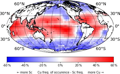
9634               J. Mohrmann et al.: Identifying meteorological influences on marine low-cloud mesoscale morphology

Figure 4. Cloud radiative properties by cloud type: (a) CERES cloud fraction, (b) cloud frequency of occurrence, (c) average CERES net
CRE per cloud type, (d) frequency-weighted net CRE. Each set of three symbols is for the 3 years (2014–2016) used. For panels (a) and (c),
the mesoscale, synoptic, climatological averages are shown using circular, diamond, and square symbols, respectively (see Sect. 2e).

common cloud type in that region and then from the top two             image on which the classifications are carried out (see Yuan
most common, etc. This is shown in Fig. 6. Figure 6a shows             et al., 2020, for additional details on classification).
the fraction of scenes covered by the dominant cloud type                 The scene selected highlights suppressed and clustered
for that grid box. In Fig. 6b, we see that in the northwest-           types. In Fig. 7a, a roughly 200 km by 400 km region of
ern corner of our region of interest, the top two cloud types          enhanced cloud in the lower middle of the scene is identi-
(in this case, suppressed and clustered Cu) account for more           fied as clustered Cu, surrounded by suppressed-Cu scenes.
than 90 % of all scenes. This suggests that any further dif-           A misidentification of sun glint as solid stratus is evident
ferentiation into more specific cloud subtypes would be most           as well (though Fig. 3 shows that very few misidentifica-
effective if focused on this region. Figure 6c and d show that         tions of this type occur in tropical scenes to have a signif-
the region with the greatest variability in cloud type is the          icant impact on the classification climatology). Figure 7b
zonal band near 45◦ S as well as the subtropical Sc–Cu tran-           and c show the surface divergence as inferred from AS-
sition region near 15◦ S.                                              CAT and the MERRA-2 reanalysis; the ASCAT overpass
                                                                       time at 09:30 LT, being 4 h ahead of the MODIS-Aqua ob-
                                                                       servation time, causes a slight geographic mismatch. Nev-
3.2    Sample case
                                                                       ertheless, both surface divergence plots show strong con-
                                                                       vergence (in blue) in the clustered region and divergence
To better illustrate the scale at which the classifications and        in surrounding regions. Note also the noisy nature of the
the underlying data exist, Fig. 7 shows a case study from              ASCAT observations as well as the narrow swath of AS-
22 July 2015. Each panel shows the classifications in col-             CAT not allowing matches with many (approximately half)
ored circles, marking the center of each rectangular MODIS

Atmos. Chem. Phys., 21, 9629–9642, 2021                                                   https://doi.org/10.5194/acp-21-9629-2021
J. Mohrmann et al.: Identifying meteorological influences on marine low-cloud mesoscale morphology 9635
Figure 5. Same as Fig. 4a but for (a) MERRA-2 sea surface temperature, (b) MERRA-2 estimated inversion strength (EIS), (c) MERRA-2
700 hPa divergence, and (d) MERRA-2 700 hPa relative humidity.
of the classifications. Figure 7f shows the large-scale diver- gle to clearly identify a scene as suppressed or clustered;
gence as inferred from the 700 hPa vertical motion. Although however on aggregate the machine learning classifications
there is some convergence aloft at the southern boundary are consistent with human labeling, as the performance eval-
of the scene (where the MERRA-2 surface convergence uation presented in Yuan et al. (2020) has shown.
is strongest), the remainder of the clustered region shows
slightly enhanced subsidence aloft, in contrast to surface 3.3 Radiative properties of morphological cloud types
conditions, which as we see later is also the mean behav-
ior for clustered scenes. MODIS indicates cloud top pres- As the climatological relevance of marine low clouds re-
sures between 800 and 700 hPa (not shown) at around 15◦ N, lates in large part to their radiative effect, it is worth iden-
138◦ W (where the divergence is strongest), consistent with tifying the variability in radiative properties among the dif-
the schematic model in BB17 (their Fig. 10). This divergence ferent categories. Figure 4 shows the low-cloud fraction of
may potentially represent the outflow from the aggregated each cloud type, with closed MCC having the highest and
convection in this clustered region. suppressed Cu the lowest. The mean cloud fraction across
Figure 7d and e show the AMSR-2 precipitation and mois- all scenes (black dot at right of Fig. 4a) also shows that the
ture retrievals, respectively. The clustered (suppressed) clas- Cu vs. Sc cloud types also split tidily into the below-average
sifications are consistently associated with a moist (dry) and above-average cloudy scenes for this particular sample,
CWV anomaly, and precipitation is only found in the clus- as expected. The mesoscale cloud fraction anomaly (repre-
tered regions. Overall, the mesoscale anomalies are clearly sented by the difference between the small diamonds and
resolved on the spatial scales of the classifications. Classifi- circles for each type) shows that, on average, the scenes we
cation edge cases exist where a human observer would strug- classify are slightly cloudier than their surroundings. This is
most pronounced for the closed MCC and most likely a re-
https://doi.org/10.5194/acp-21-9629-2021 Atmos. Chem. Phys., 21, 9629–9642, 20219636 J. Mohrmann et al.: Identifying meteorological influences on marine low-cloud mesoscale morphology
quently occurring in our dataset, due to their dominance in
the tropics and subtropics, one should keep in mind that their
low mean instantaneous CRE is counterbalanced by their
high frequency of occurrence. The frequency-weighted CRE
(Fig. 4d), which is simply the product for each year of the
data in Fig. 4b and c, is therefore appropriate as it represents
the fraction of total cooling, over all scenes, by a particu-
lar cloud type. Thus open MCC, despite having a mean net
CRE of −100 W m−2 , only accounts for ∼ 5 W m−2 of the
total cooling of all scenes in our dataset (approximately 4 %);
while these scenes have high CFs and therefore net CRE,
they are infrequent, more so in this classification compared
to previous work. For the clustered and suppressed types, the
importance of understanding their drivers is highlighted in
Fig. 4d; clustered-Cu scenes have a contribution to the net
CRE that is 5 times higher than suppressed-Cu scenes.
3.4 Composite analysis
Figure 6. The fraction of cloud scenes for each grid point, which
are represented by (a) the most common cloud type for that grid
point and (b–d) the top two through top four most common cloud Figures 5 and 8 are similar to Fig. 4, showing composites
types. Gray areas indicate that fewer than 200 scenes were sampled. of meteorological variables by cloud type as well as synop-
tic and climatological averages (where seasonal mean values
for a given location are composited instead of instantaneous
values). For both these figures, we can estimate the variabil-
sult of the filtering of scenes with very low cloud. The only ity between types explained by differences in geography by
exception is suppressed Cu, which is associated with a low comparing the mesoscale averages (circles) to the climato-
CF anomaly. The same is true when comparing to the clima- logical averages (squares). For instance, for every cloud type,
tological cloud fraction (small squares) where a high bias in there is almost no bias between the mesoscale and climato-
cloud fraction is seen, again most likely due to the fact that logical averages of sea surface temperature (SST; Fig. 5a).
we can only classify cloudy scenes. In other words, variation in SST between scenes is almost
Figure 4b–d show the composite net CRE of the various entirely explainable by the variation in geography. The sup-
cloud types. In Fig. 4b the overall frequency of each cloud pressed scenes occur over the warmest waters and the closed
type in our dataset is broken down by year (2014–2016). MCC over the coldest. The same is largely true for EIS,
Together, clustered- and suppressed-Cu scenes account for which is determined in part by SST. This is not surprising
more than half of all scenes. Figure 4c shows the CERES given the geographic distributions of the cloud types seen
net CRE as calculated in Sect. 2b for each type and year earlier and climatological gradients in SST and EIS. What
as well as the mesoscale and climatological value. The net this tells us, however, is that there is no strong evidence
CRE, mostly coming from the shortwave, broadly mirrors for subseasonal timescale perturbations to SST or EIS co-
the cloud fraction. The total cooling averaged over all scenes inciding with variations in cloud type. We can also compare
is shown as the black dots in Fig. 4c, corresponding to a net the mesoscale averages to the 10◦ synoptic averages to as-
CRE of ∼ −113 W m−2 . Note that due to the specific sam- sess whether any mesoscale anomalies are coincident with
pling strategy (only considering scenes with low cloud, with- cloud type variability. However, an important caveat to bear
out too much overlying high cloud) and the fact that we com- in mind is the bias introduced by our sampling strategy: only
posite instantaneous daytime values that are not weighted by scenes with some low cloud and not too much high cloud are
the global frequency of occurrence of our cloud types, our considered, whereas the surrounding scenes are not similarly
CRE for marine low clouds is approximately an order of constrained. These biases are best identified from the black
magnitude larger than the global value found by L’Ecuyer “all scenes” markers. For instance, we notice in Fig. 5d that
et al. (2019). averaged over all scenes, RH700 is biased low by 3 %, most
The above difference between instantaneous local and likely due to preferential selection of scenes with little high
global values underscores the fact that when considering the cloud (and therefore a free troposphere that is biased dry).
radiative importance of different cloud types, both frequency This bias is also applicable to the climatological compari-
and mean CRE at the time of occurrence are relevant. Specif- son. The dry free troposphere (FT) anomaly relative to the
ically, when considering the Cu cloud types (clustered and synoptic (and climatological) averages in, for example, the
suppressed), which are the two types that are the most fre- closed-MCC scenes can be explained by this sampling bias
Atmos. Chem. Phys., 21, 9629–9642, 2021 https://doi.org/10.5194/acp-21-9629-2021J. Mohrmann et al.: Identifying meteorological influences on marine low-cloud mesoscale morphology 9637
Figure 7. Sample region observed on 22 July 2015 showing classifications (every panel, in colored circles). (a) MODIS true-color reflectance,
(b) ASCAT surface divergence, (c) MERRA-2 surface divergence, (d) AMSR-2 89 Ghz precipitation rate, (e) AMSR-2 column water vapor,
(f) MERRA-2 700 hPa divergence.
and is not indicative of some mechanism in a drier FT yield- Composite analysis of the surface divergence, however, is
ing closed-MCC clouds. much more helpful at distinguishing between the Cu cloud
With that caveat in mind, Fig. 5 shows that closed MCC types. This is evident from Fig. 8a and b. From the ASCAT
and to a lesser extent disorganized MCC are associated with composite data, the strongest surface divergence is associ-
a significant mesoscale anomaly in EIS (consistent with ated with suppressed scenes and the strongest convergence
Muhlbauer et al., 2014). Solid stratus is associated with a with the clustered scenes. When using MERRA-2 data, the
positive anomaly in vertical motion and RH700 relative to only difference is that the closed-MCC cases have slightly
climatology but not a mesoscale one, indicating that this link stronger divergence, yet the clear separation between Cu
is driven by synoptic features; manual inspection confirms types remains. Additionally, the surface divergence signal is
that many scenes identified as stratus are indeed associated clearly of a mesoscale nature and not explained by climato-
with frontal systems. Both closed and open MCC are asso- logical differences, particularly for the convergence associ-
ciated with strong subseasonal anomalies of enhanced subsi- ated with clustered scenes; the synoptic environment shows
dence, though again the absence of an anomaly relative to the broad divergence.
synoptic mean indicates that these are larger features, likely Having calculated both the 700 hPa large-scale and sur-
associated with variability in the position of the subtropical face divergence, we can subtract the former from the latter
high. to estimate a boundary layer anomaly divergence. If near-
Aside from the mesoscale and subseasonal anomaly anal- surface divergence purely reflects the large-scale subsiding
ysis, a key result is that clustered and suppressed types are flow, with no additional low-level circulation, we would ex-
poorly separated by the variables in Fig. 5; they have virtually pect this anomaly to be small. Figure 9a shows this surface
identical EIS distributions, and though suppressed scenes are level anomaly using both the MERRA-2 and ASCAT winds.
associated with slightly higher SST, large-scale divergence, The large positive anomaly for suppressed-Cu scenes indi-
and lower FT humidity, there is not much separation between cates that the bulk of the divergence is a result of near-surface
them in this phase space, especially relative to the variabil- circulations rather than those extending over a deep layer of
ity between all cloud types, and these small differences are the lower troposphere; similarly for clustered Cu, the surface
consistent with their slightly different geographic distribu- convergence together with mean large-scale divergence indi-
tions. In contrast, EIS is an excellent discriminator between cates a shallow circulation, as seen in the case study of Fig. 7.
the stratiform MCC types. Considering AMSR-2 retrievals, the rain rate shows a
very clear separation between clustered and suppressed cloud
https://doi.org/10.5194/acp-21-9629-2021 Atmos. Chem. Phys., 21, 9629–9642, 20219638 J. Mohrmann et al.: Identifying meteorological influences on marine low-cloud mesoscale morphology
Figure 8. Same as Fig. 5 but with (a) ASCAT surface wind divergence, (b) MERRA-2 surface wind divergence, (c) AMSR-2 rain rate, and
(d) AMSR-2 column water vapor.
types, with a strong positive (negative) mesoscale anomaly that the higher mean state moisture in BB17 would occur
for clustered (suppressed) Cu of around 0.4 mm d−1 . Simi- with larger moisture anomalies.
lar qualitative results are found for conditional rain rates and
rain probabilities (not shown). It is worth noting that the res- 3.5 Aircraft observations
olution of the precipitation data is approximately 4 km, so
the smallest clouds will not be resolved. The column wa- Figure 10 shows the depth of the boundary layer and degree
ter vapor results are interesting as well; consistent with the of decoupling (using the αq metric from Wood and Brether-
warm SSTs, both Cu cloud types occur in areas of high ton, 2004) based on CSET aircraft profiles. The parameter αq
column water vapor. The mesoscale anomalies, however, is a measure of relative resemblance of upper-boundary-layer
are consistent with the BB17 presentation: clustered scenes moisture to the lower FT and lower boundary layer, with a
are slightly moister than their environment and suppressed value of 0 indicating a perfectly well-mixed boundary layer
scenes slightly drier. This is difficult to identify in Fig. 8d, and a value of 1 indicating a perfectly decoupled boundary
so Fig. 9b shows just the mesoscale anomaly for all cloud layer, where the upper-boundary-layer moisture is equal to
types and makes clear that the suppressed scenes are the most the lower FT moisture.
anomalously dry and the clustered scenes most anomalously qT (upper BL) − qT (lower BL)
moist. Although the moisture anomalies of the LES in BB17 αqT = (3)
qT (lower FT) − qT (lower BL)
were larger than those found here, this may be due to their
mean state being moister. One finding from that work is that For a given profile, the thermal inversion height is estimated
the amplitude of aggregation-associated moisture anomalies using the maximum lapse rate, with the inversion being the
tended to scale with the mean state CWV, and so we expect layer where the lapse rate deviation from a moist adiabat ex-
ceeds 25 % of maximum deviation (this was tuned to agree
Atmos. Chem. Phys., 21, 9629–9642, 2021 https://doi.org/10.5194/acp-21-9629-2021J. Mohrmann et al.: Identifying meteorological influences on marine low-cloud mesoscale morphology 9639
Figure 9. (a) Surface divergence anomaly from 700 hPa (circles are based on MERRA-2 surface winds; squares are based on ASCAT surface
winds). (b) AMSR-2 column water vapor mesoscale anomaly.
and so the full histograms are shown (smoothed using ker-
nel density estimation) to highlight the uncertainty. Adopt-
ing a Lagrangian perspective, which accounts for the bound-
ary layer evolving downstream of the trade winds through
the Sc–Cu transition, boundary layer deepening and decou-
pling are found from stratus through closed, disorganized,
and open MCC; in particular the degree of decoupling be-
tween closed and open MCC is very pronounced, with the
former being the most coupled and the latter the most decou-
pled. However, this evolution breaks down for the Cu-type
boundary layers, which are neither deeper nor more decou-
pled than open MCC. This is not surprising as the inversion
Figure 10. Histograms of (a) boundary layer depth and (b) bound- at the top of the surface mixed layer where Cu clouds form
ary layer decoupling index from CSET flights and dropsonde obser- will persist as the decoupled Sc layer is eroded, such that the
vations. remaining boundary layer stays shallower and strongly cou-
pled to the surface. Also important to note is that, as with
EIS and SST, clustered and suppressed types are difficult to
with a visual assessment of the inversion layer and worked distinguish by their depth and decoupling state, though clus-
well for all profiles). Upper and lower BL in the qT equation tered scenes are marginally deeper in Fig. 10a.
are taken as the top and bottom 25 % of the BL depth, while
the lower FT starts 500 m above the inversion top. While this
method may not be the most precise in individual, more com- 4 Conclusions
plex cumulus cases with more spatially and vertically het-
erogeneous moisture profiles, we use it for consistency and In this study we have analyzed the characteristics of the ma-
reproducibility. We also note that a joint histogram analysis rine boundary layer for six different morphological cloud
of αq vs. cloud layer depth (not shown) produced consistent types, the occurrence of which was derived by novel machine
results to Wood and Bretherton (2004) and Park et al. (2004). learning-based cloud classification operating on MODIS
For each aircraft profile, the cloud type classification mesoscale imagery. Specifically, we assessed whether the
which covers that profile is selected for compositing, and observations of clustered and suppressed cumulus are con-
so the profile represents a random estimate of depth or de- sistent with previous modeling of mesoscale aggregation of
coupling within that scene. Here the sample sizes are much shallow cumulus. The key findings are as follows:
smaller than the composites of satellite and reanalysis data,
https://doi.org/10.5194/acp-21-9629-2021 Atmos. Chem. Phys., 21, 9629–9642, 20219640 J. Mohrmann et al.: Identifying meteorological influences on marine low-cloud mesoscale morphology
– The six cloud types represent distinct MBL regimes, be seen whether the process of shallow convective aggrega-
based on their geography and environmental conditions. tion affects synoptic-scale mean cloud cover and CRE. Given
that models capable of reproducing such shallow aggregation
– The anomalies in cloudiness, column water vapor, are now able to run at global scales (Bretherton and Khairout-
circulation, and precipitation are consistent with the dinov, 2015), this question is best answered using simulation
Bretherton and Blossey (2017) LES results and concep- studies.
tual model for mesoscale shallow aggregation.
– Suppressed- and clustered-Cu scenes are most clearly Data availability. MODIS reflectance data for this work are
separable by looking at surface wind divergence, and available at https://doi.org/10.5067/MODIS/MYD021KM.006
this signal is apparent in both satellite retrievals and the (MCST/MODAPS, 2016). ASCAT data are available from
MERRA-2 reanalysis. http://www.remss.com/missions/ascat/ (last access: 2 Decem-
ber 2019) (Ricciardulli and Wentz, 2016). AMSR-2 water vapor
data are available at http://www.remss.com/missions/amsr/
This last finding pertains to a more general conclusion,
(Wentz et al., 2014). CERES SYN1deg data are avail-
namely that, at least for the variables considered, mesoscale able at https://doi.org/10.1175/JTECH-D-12-00136.1
anomalies in meteorological variables are more pronounced (Doelling et al., 2013). MERRA-2 data are available at
for the cumulus types than the stratiform MCC types; this https://doi.org/10.5067/QBZ6MG944HW0 (GMAO, 2015). CSET
is true for CWV, precipitation, and surface divergence. For aircraft data are available at https://doi.org/10.5065/D65Q4T96
discriminating between the MCC types, EIS, depth, and de- (UCAR/NCAR EOL, 2017). Data processing code as well
coupling are the most useful; in stratocumulus regions, these as processed classification data can be found on Zenodo at
variables have been shown to correlate strongly with each https://doi.org/10.5281/zenodo.4673556 (Mohrmann, 2021).
other and with cloud cover (Wood and Bretherton, 2004;
Wood and Hartmann, 2006).
Though it is tempting to conclude that surface divergence Author contributions. JM prepared the manuscript and performed
is such a good discriminator because the mesoscale aggre- most of the data analysis. RW provided continuous feedback and
guidance during the analysis. TY and HS were responsible for
gation described in BB17 is likely the most important deter-
the creation and processing of the classification dataset. RE pro-
minant of cloud variability, we must also bear in mind that,
vided the AMSR brightness temperature dataset and guidance on its
along with precipitation, it is more an “internal” boundary proper use and interpretation. TY, HS, JM, RW, and LO all partici-
layer predictor than most of the other predictors, e.g., EIS pated in the development of the classification methodology and sub-
or SST, and therefore better coupled to other MBL state vari- sequent interpretation and refinement of the classification dataset.
ables (e.g., cloud fraction). Additionally, it is also much more All coauthors provided editorial feedback on the manuscript.
directly observed and resolved at a finer scale than, for ex-
ample, 700 hPa vertical motion and therefore has a lower ob-
servational uncertainty. That being said, the strong consis- Competing interests. The authors declare that they have no conflict
tency between the observations and the BB17 LES modeling of interest.
of mesoscale shallow convection suggests that this process is
an important driver of cumulus-dominated MBL cloud vari-
ability. Acknowledgements. We gratefully acknowledge our colleagues at
There are several limitations on the generalizability of the University of Washington for feedback and helpful discussion.
these results. The first is that we have only considered the Funding for this research was provided in part by the NASA MEa-
SUREs program. We acknowledge the use of imagery from the
SEP and NEP regions, and other clouds, particularly those in
NASA Worldview application (https://worldview.earthdata.nasa.
the warmer trade wind regions of the western ocean basins, gov/, last access: 26 May 2020), part of the NASA Earth Observing
may have different MBL characteristics. The second is that System Data and Information System (EOSDIS). We are also very
we have only considered daytime behavior and cannot ac- grateful to the anonymous reviewers for their valuable feedback,
count for diurnal variability in cloud type. The observations both scientific and editorial.
from aircraft data were limited and did not extend south of
Hawaii or north of California. Lastly, we have not examined
in depth the role of SST in determining cloud type. This is Financial support. This research has been supported by
not because it is unimportant (on the contrary, it is a key the National Aeronautics and Space Administration (grant
driver of most MCC variability; see McCoy et al., 2017) but no. 80NSSC18M0084).
rather because it does not vary much at mesoscale and short
timescales.
With regards to climate modeling, CRE for different cloud Review statement. This paper was edited by Yafang Cheng and re-
types largely mirrors cloud fraction. While the CRE between viewed by two anonymous referees.
suppressed and clustered types is very different, it remains to
Atmos. Chem. Phys., 21, 9629–9642, 2021 https://doi.org/10.5194/acp-21-9629-2021J. Mohrmann et al.: Identifying meteorological influences on marine low-cloud mesoscale morphology 9641
References Hahn, C. J., Rossow, W. B., and Warren, S. G.: IS-
CCP Cloud Properties Associated with Standard Cloud
Agee, E. M.: Mesoscale cellular convection over the oceans, Dy- Types Identified in Individual Surface Observations,
nam. Atmos. Ocean., 10, 317–341, https://doi.org/10.1016/0377- J. Climate, 14, 11–28, https://doi.org/10.1175/1520-
0265(87)90023-6, 1987. 0442(2001)0142.0.CO;2, 2001.
Albrecht, B., Ghate, V., Mohrmann, J., Wood, R., Zuidema, P., Hartmann, D. L., Ockert-Bell, M. E., and Michelsen, M. L.: The
Bretherton, C., Schwartz, C., Eloranta, E., Glienke, S., Don- Effect of Cloud Type on Earth’s Energy Balance: Global Anal-
aher, S., Sarkar, M., McGibbon, J., Nugent, A. D., Shaw, R. ysis, J. Climate, 5, 1281–1304, https://doi.org/10.1175/1520-
A., Fugal, J., Minnis, P., Paliknoda, R., Lussier, L., Jensen, J., 0442(1992)0052.0.CO;2, 1992.
Vivekanandan, J., Ellis, S., Tsai, P., Rilling, R., Haggerty, J., L’Ecuyer, T. S., Hang, Y., Matus, A. V., and Wang, Z.: Re-
Campos, T., Stell, M., Reeves, M., Beaton, S., Allison, J., Stoss- assessing the Effect of Cloud Type on Earth’s Energy Bal-
meister, G., Hall, S., and Schmidt, S.: Cloud System Evolution in ance in the Age of Active Spaceborne Observations. Part I:
the Trades (CSET): Following the Evolution of Boundary Layer Top of Atmosphere and Surface, J. Climate, 32, 6197–6217,
Cloud Systems with the NSF–NCAR GV, B. Am. Meteorol. https://doi.org/10.1175/JCLI-D-18-0753.1, 2019.
Soc., 100, 93–121, https://doi.org/10.1175/BAMS-D-17-0180.1, LeMone, M. A. and Meitin, R. J.: Three Examples of Fair-Weather
2019. Mesoscale Boundary-Layer Convection in the Tropics, Mon.
Bretherton, C. S. and Blossey, P. N.: Understanding Mesoscale Weather Rev., 112, 1985–1998, https://doi.org/10.1175/1520-
Aggregation of Shallow Cumulus Convection Using Large- 0493(1984)1122.0.CO;2, 1984.
Eddy Simulation, J. Adv. Model. Earth Syst., 9, 2798–2821, McCoy, I. L., Wood, R., and Fletcher, J. K.: Identifying Me-
https://doi.org/10.1002/2017MS000981, 2017. teorological Controls on Open and Closed Mesoscale
Bretherton, C. S. and Khairoutdinov, M. F.: Convective self- Cellular Convection Associated with Marine Cold Air
aggregation feedbacks in near-global cloud-resolving simula- Outbreaks, J. Geophys. Res.-Atmos., 122, 11678–11702,
tions of an aquaplanet, J. Adv. Model. Earth Syst., 7, 1765–1787, https://doi.org/10.1002/2017JD027031, 2017.
https://doi.org/10.1002/2015MS000499, 2015. MCST/MODAPS – Characterization Support Team/MODIS
Chen, T., Rossow, W. B., and Zhang, Y.: Radia- Adaptive Processing System: MODIS/Aqua Cali-
tive Effects of Cloud-Type Variations, J. Cli- brated Radiances 5-Min L1B Swath 1 km, Dataset,
mate, 13, 264–286, https://doi.org/10.1175/1520- https://doi.org/10.5067/MODIS/MYD021KM.006, 2016.
0442(2000)0132.0.CO;2, 2000. Mohrmann, J: jkcm/mesoscale-morphology: (Version 1.0), Zenodo,
Doelling, D. R., Loeb, N. G., Keyes, D. F., Nordeen, M. L., https://doi.org/10.5281/zenodo.4673556, 2021.
Morstad, D., Nguyen, C., Wielicki, B. A., Young, D. F., and Mohrmann, J., Bretherton, C. S., McCoy, I. L., McGibbon, J.,
Sun, M.: Geostationary Enhanced Temporal Interpolation for Wood, R., Ghate, V., Albrecht, B., Sarkar, M., Zuidema, P., and
CERES Flux Products, J. Atmos. Ocean. Tech., 30, 1072–1090, Palikonda, R.: Lagrangian Evolution of the Northeast Pacific Ma-
https://doi.org/10.1175/JTECH-D-12-00136.1, 2013. rine Boundary Layer Structure and Cloud during CSET, Mon.
Eastman, R., Lebsock, M., and Wood, R.: Warm Rain Rates Weather Rev., 147, 4681–4700, https://doi.org/10.1175/MWR-
from AMSR-E 89-GHz Brightness Temperatures Trained Using D-19-0053.1, 2019.
CloudSat Rain-Rate Observations, J. Atmos. Ocean. Tech., 36, Muhlbauer, A., McCoy, I. L., and Wood, R.: Climatology of
1033–1051, https://doi.org/10.1175/JTECH-D-18-0185.1, 2019. stratocumulus cloud morphologies: microphysical properties
Emanuel, K., Wing, A. A., and Vincent, E. M.: Radiative- and radiative effects, Atmos. Chem. Phys., 14, 6695–6716,
convective instability, J. Adv. Model. Earth Syst., 6, 75–90, https://doi.org/10.5194/acp-14-6695-2014, 2014.
https://doi.org/10.1002/2013MS000270, 2014. Nicholls, S. D. and Young, G. S.: Dendritic Patterns in Tropical
Gelaro, R., McCarty, W., Suárez, M. J., Todling, R., Molod, A., Cumulus: An Observational Analysis, Mon. Weather Rev., 135,
Takacs, L., Randles, C. A., Darmenov, A., Bosilovich, M. G., Re- 1994–2005, https://doi.org/10.1175/MWR3379.1, 2007.
ichle, R., Wargan, K., Coy, L., Cullather, R., Draper, C., Akella, Park, S., Leovy, C. B., and Rozendaal, M. A.: A New Heuristic La-
S., Buchard, V., Conaty, A., da Silva, A. M., Gu, W., Kim, G. grangian Marine Boundary Layer Cloud Model, J. Atmos. Sci.,
K., Koster, R., Lucchesi, R., Merkova, D., Nielsen, J. E., Par- 61, 3002–3024, https://doi.org/10.1175/JAS-3344.1, 2004.
tyka, G., Pawson, S., Putman, W., Rienecker, M., Schubert, S. Platnick, S., Meyer, K. G., King, M. D., Wind, G., Amarasinghe, N.,
D., Sienkiewicz, M., and Zhao, B.: The modern-era retrospective Marchant, B., Arnold, G. T., Zhang, Z., Hubanks, P. A., Holz, R.
analysis for research and applications, version 2 (MERRA-2), E., Yang, P., Ridgway, W. L., and Riedi, J.: The MODIS Cloud
J. Climate, 30, 5419–5454, https://doi.org/10.1175/JCLI-D-16- Optical and Microphysical Products: Collection 6 Updates and
0758.1, 2017. Examples From Terra and Aqua, IEEE T. Geosci. Remote, 55,
GMAO – Global Modeling and Assimilation Office: MERRA- 502–525, https://doi.org/10.1109/TGRS.2016.2610522, 2017.
2 inst3_3d_asm_Np: 3d,3-Hourly,Instantaneous,Pressure- Ricciardulli, L. and Wentz, F. J.: Remote Sensing Systems AS-
Level,Assimilation,Assimilated Meteorological Fields V5.12.4, CAT C-2015 Daily Ocean Vector Winds on 0.25 deg grid, ver-
GES DISC – Goddard Earth Sciences Data and In- sion 02.1, Remote Sens. Syst., St. Rosa, CA, available at: http://
formation Services Center, Greenbelt, MD, USA, www.remss.com/missions/ascat/ (last access: 2 December 2019),
https://doi.org/10.5067/QBZ6MG944HW0, 2015. 2016.
Hahn, C. J. and Warren, S. G.: A Gridded Climatology of Clouds Stevens, B., Bony, S., Brogniez, H., Hentgen, L., Hohenegger,
over Land (1971–1996) and Ocean (1954–2008) from Sur- C., Kiemle, C., L’Ecuyer, T. S., Naumann, A. K., Schulz, H.,
face Observations Worldwide (NDP-026E), OSTI dataset, USA, Siebesma, P. A., Vial, J., Winker, D. M., and Zuidema, P.:
https://doi.org/10.3334/CDIAC/CLI.NDP026E, 2007.
https://doi.org/10.5194/acp-21-9629-2021 Atmos. Chem. Phys., 21, 9629–9642, 20219642 J. Mohrmann et al.: Identifying meteorological influences on marine low-cloud mesoscale morphology Sugar, gravel, fish and flowers: Mesoscale cloud patterns in Wood, R. and Bretherton, C. S.: On the Relationship between Strati- the trade winds, Q. J. Roy. Meteorol. Soc., 146, 141–152, form Low Cloud Cover and Lower-Tropospheric Stability, J. Cli- https://doi.org/10.1002/qj.3662, 2020. mate, 19, 6425–6432, https://doi.org/10.1175/JCLI3988.1, 2006. UCAR/NCAR EOL – Earth Observing Laboratory: Low Rate (LRT Wood, R. and Hartmann, D. L.: Spatial variability of liq- – 1 sps) Navigation, State Parameter, and Microphysics Flight- uid water path in marine low cloud: The importance of Level Data, Version 1.2, UCAR/NCAR – Earth Observing Lab- mesoscale cellular convection, J. Climate, 19, 1748–1764, oratory, https://doi.org/10.5065/D65Q4T96, 2017. https://doi.org/10.1175/JCLI3702.1, 2006. Warren, S. G., Hahn, C. J., London, J., Chervin, R. M., and Jenne, Wood, R., Köhler, M., Bennartz, R., and O’Dell, C.: The diurnal R. L.: Global distribution of total cloud cover and cloud type cycle of surface divergence over the global oceans, Q. J. Roy. amounts over the ocean, NCAR Technical Note, NCAR-TN 317, Meteorol. Soc., 135, 1484–1493, https://doi.org/10.1002/qj.451, https://doi.org/10.2172/5415329, 1988. 2009. Wentz, F. J., Meissner, T., Gentemann, C., Hilburn, K. A., and Yuan, T., Song, H., Wood, R., Mohrmann, J., Meyer, K., Ore- Scott, J.: Remote Sensing Systems GCOM-W1 AMSR2 Daily opoulos, L., and Platnick, S.: Applying deep learning to NASA Environmental Suite on 0.25 deg grid, version 8, Remote MODIS data to create a community record of marine low-cloud Sens. Syst., St. Rosa, CA, available at: http://www.remss.com/ mesoscale morphology, Atmos. Meas. Tech., 13, 6989–6997, missions/amsr/ (last access: 29 January 2020), 2014. https://doi.org/10.5194/amt-13-6989-2020, 2020. Wood, R. and Bretherton, C. S.: Boundary Layer Depth, Entrainment, and Decoupling in the Cloud-Capped Subtropical and Tropical Marine Boundary Layer, J. Climate, 17, 3576–3588, https://doi.org/10.1175/1520- 0442(2004)0172.0.CO;2, 2004. Atmos. Chem. Phys., 21, 9629–9642, 2021 https://doi.org/10.5194/acp-21-9629-2021
You can also read