Analytical solution for residual stress and strain preserved in anisotropic inclusion entrapped in an isotropic host
←
→
Page content transcription
If your browser does not render page correctly, please read the page content below
Solid Earth, 12, 817–833, 2021
https://doi.org/10.5194/se-12-817-2021
© Author(s) 2021. This work is distributed under
the Creative Commons Attribution 4.0 License.

Analytical solution for residual stress and strain preserved in
anisotropic inclusion entrapped in an isotropic host
Xin Zhong1,2 , Marcin Dabrowski2,3 , and Bjørn Jamtveit2
1 Institut
        für Geologische Wissenschaften, Freie Universität Berlin, Malteserstrasse 74–100, 12449 Berlin, Germany
2 Physicsof Geological Processes, The Njord Center, University of Oslo, Oslo, Norway
3 Computational Geology Laboratory, Polish Geological Institute – NRI, Wrocław, Poland

Correspondence: Xin Zhong (xinzhong0708@gmail.com)

Received: 19 October 2020 – Discussion started: 26 October 2020
Revised: 9 January 2021 – Accepted: 16 February 2021 – Published: 15 April 2021

Abstract. Raman elastic thermobarometry has recently been            inclusion and the analytically calculated stress from the best-
applied in many petrological studies to recover the pressure         fitted effective ellipsoid is calculated to obtain the root-mean-
and temperature (P –T ) conditions of mineral inclusion en-          square deviation (RMSD) for quartz, zircon, rutile, apatite,
trapment. Existing modelling methods in petrology either             and diamond inclusions in garnet host. Based on the results
adopt an assumption of a spherical, isotropic inclusion em-          of 500 randomly generated (a wide range of aspect ratio and
bedded in an isotropic, infinite host or use numerical tech-         random crystallographic orientation) faceted inclusions, we
niques such as the finite-element method to simulate the             show that the volumetrically averaged stress serves as an ex-
residual stress and strain state preserved in the non-spherical      cellent stress measure and the associated RMSD is less than
anisotropic inclusions. Here, we use the Eshelby solution to         2 %, except for diamond, which has a systematically higher
develop an analytical framework for calculating the residual         RMSD (ca. 8 %). This expands the applicability of the ana-
stress and strain state of an elastically anisotropic, ellipsoidal   lytical solution for any arbitrary inclusion shape in practical
inclusion in an infinite, isotropic host. The analytical solution    Raman measurements.
is applicable to any class of inclusion symmetry and an arbi-
trary inclusion aspect ratio. Explicit expressions are derived
for some symmetry classes, including tetragonal, hexagonal,
and trigonal.                                                        1   Introduction
   The effect of changing the aspect ratio on residual stress is
investigated, including quartz, zircon, rutile, apatite, and dia-    Raman elastic thermobarometry has been extensively used
mond inclusions in garnet host. Quartz is demonstrated to be         to recover the pressure and temperature (P –T ) conditions of
the least affected, while rutile is the most affected. For pro-      mineral inclusion entrapment, e.g. the mostly studied quartz-
late quartz inclusion (c axis longer than a axis), the effect of     in-garnet inclusion–host pair (Ashley et al., 2014; Bayet et
varying the aspect ratio on Raman shift is demonstrated to be        al., 2018; Enami et al., 2007; Gonzalez et al., 2019; Kouketsu
insignificant. When c/a = 5, only ca. 0.3 cm−1 wavenumber            et al., 2014; Taguchi et al., 2016, 2019; Zhong et al., 2019).
variation is induced as compared to the spherical inclusion          Recently, quartz-in-garnet elastic barometry has been cali-
shape. For oblate quartz inclusions, the effect is more signif-      brated with experiments by synthesizing almandine garnets
icant, when c/a = 0.5, ca. 0.8 cm−1 wavenumber variation             and quartz inclusions at high P –T conditions and compar-
for the 464 cm−1 band is induced compared to the reference           ing the entrapment pressure recovered based on the residual
spherical inclusion case. We also show that it is possible to        pressure measured in quartz with the pressure applied in ex-
fit an effective ellipsoid to obtain a proxy for the averaged        periments (Bonazzi et al., 2019; Thomas and Spear, 2018).
residual stress or strain within a faceted inclusion. The differ-    In practice, most mineral inclusions, e.g. quartz, zircon, and
ence between the volumetrically averaged stress of a faceted         rutile, are elastically anisotropic, and the associated effect
                                                                     needs to be addressed to better constrain the entrapment P –

Published by Copernicus Publications on behalf of the European Geosciences Union.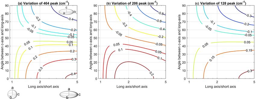
818                                                         X. Zhong et al.: Analytical solution for residual stress and strain

T conditions. Existing mechanical models for elastic ther-         ual stress and strain are derived. The analytical formulas are
mobarometry typically treat the case of a spherical isotropic      cross-validated against the numerical results obtained using
inclusion entrapped in an infinite, isotropic host (e.g. Angel     a self-developed finite-element code. Convergence tests are
et al., 2017; Gillet et al., 1984; Guiraud and Powell, 2006;       successfully performed to show the correspondence of the
Rosenfeld and Chase, 1961; Zhang, 1998). In recent stud-           numerical (FE) and analytical solutions. In-depth analysis of
ies, finite-element (FE) simulations were applied to study         the effects due to (1) inclusion elastic anisotropy, (2) inclu-
anisotropic inclusions entrapped in cubic hosts such as gar-       sion aspect ratio, and (3) relative orientation between the in-
net (Alvaro et al., 2020; Mazzucchelli et al., 2019). In this      clusion crystallographic and geometrical principal axes are
approach, the residual strain preserved within a mineral in-       performed to show how they affect the application of elastic
clusion is related to the stress and strain state of the system    thermobarometry. The MATLAB code has also been made
upon entrapment via a relaxation tensor (R) that needs to be       available alongside the submission.
pre-calculated using the FE method or other numerical tech-            One major problem of using the Eshelby solution for min-
niques (Mazzucchelli et al., 2019).                                eral inclusion is that natural inclusions are faceted in shape,
   For an ellipsoidal, elastically anisotropic inclusion en-       which leads to a heterogeneous residual stress field (e.g.
trapped in an infinite isotropic host, an exact closed-form        Chiu, 1978; Mazzucchelli et al., 2018). To resolve this issue,
analytical solution has been available for a long time (Es-        we use our self-developed 3D finite-element code to simu-
helby, 1957; Mura, 1987). This solution has been widely            late the residual stress distribution within faceted inclusions
applied in Earth science for many problems, such as vis-           of varying shapes. Fitting an arbitrary 3D shape with effec-
cous creep around inclusions (Freeman, 1987; Jiang, 2016),         tive ellipsoid is a common practice in image analysis and
flanking structures (Exner and Dabrowski, 2010); elastic           microstructural research (e.g. Ghosh and Dimiduk, 2011).
stress of inclusions at various scales (Meng and Pollard,          We explore the possibility of using an effective ellipsoid to
2014), microcracking and faulting (Healy et al., 2006),            approximate the shape of a faceted inclusion. The residual
and magma-chamber-induced deformations (Bonaccorso and             stress obtained from the analytical solution based on the best-
Davis, 1999). The advantage of such an approach is that            fitted effective ellipsoid is used as a proxy to represent the
no numerical software or programming is required and the           volumetrically averaged stress within the faceted inclusion.
solution can be obtained rapidly and precisely, with no nu-        By inspecting the numerical (FE) and analytical solutions,
merical approximation error. The rapid calculation also per-       we have found that for most mineral inclusions, e.g. quartz,
mits in-depth, systematic stress and strain analysis of the        zircon, apatite, and rutile, the volumetrically averaged stress
inclusion–host system or a potential Monte Carlo simula-           represents the stress state of arbitrarily faceted inclusions
tion for uncertainty propagation. The procedure of calcu-          very well. This may potentially provide a useful guide for
lating the residual stress in an ellipsoidal anisotropic inclu-    future applications of elastic thermobarometry for any natu-
sion embedded in an elastic, isotropic host is based on the        ral faceted mineral inclusions.
equivalent eigenstrain method and the classical Eshelby so-
lution (Eshelby, 1957; Mura, 1987). Recently, the Eshelby
solution has been applied to exhumed mineral inclusions en-        2     Method
trapped in a host and the result has been compared to the
finite-element method (Morganti et al., 2020). Mineral in-         2.1    Anisotropic inclusion embedded in isotropic host
clusions were measured for their crystallographic orienta-
tion and shape via X-ray diffraction and tomography (Mor-          We consider an anisotropic, ellipsoidal solid inclusion en-
ganti et al., 2020), but the significance of the aspect ratio,     trapped in an isotropic, infinite host at high P –T conditions.
shape, and crystallographic orientation has not been stud-         For a fully entrapped spherical inclusion, the assumption of
ied in a systematic way. More importantly, the Eshelby so-         an infinite host is justified when the distance between the in-
lution only applies to perfectly ellipsoidal inclusions, but       clusion and host grain outer boundaries, such as the thin-
natural mineral inclusions are faceted. Therefore, the un-         section surface, is more than 3 times the inclusion radius
certainty in and limitations of using the Eshelby solution         (Mazzucchelli et al., 2018; Zhong et al., 2018). The prin-
for natural faceted inclusions remain to be investigated. In       cipal axes of the inclusion are aligned along the Cartesian
this study, we explore the Eshelby solution in-depth relating      coordinates x, y, and z, and their lengths are arbitrary. Upon
to the inclusion–host problem. A general analytical form is        entrapment at depth, the inclusion and host are considered
first presented in this paper (the previous submission record      subject to the same stress field. The entrapment stress may
is given in the Acknowledgements) following the Eshelby            be either hydrostatic or non-hydrostatic but it is treated as ho-
equivalent eigenstrain method (Mura, 1987, chap. 4) to cal-        mogeneous during the inclusion growth within the host grain
culate residual stress and strain of an anisotropic inclusion in   or the overgrowth of the inclusion by the host grain. At this
an isotropic host. For inclusions belonging to certain crystal-    stage, the lattice strains of the inclusion and host are denoted
lographic symmetry, such as tetragonal, hexagonal, and trig-       by εiincl and εihost , which are measured with respect to the ref-
onal classes, simplified explicit expressions describing resid-    erence room conditions. The Voigt notation is applied here

Solid Earth, 12, 817–833, 2021                                                          https://doi.org/10.5194/se-12-817-2021
X. Zhong et al.: Analytical solution for residual stress and strain                                                                      819

(Voigt, 1910). The entrapment lattice strains εiincl and εihost           find that mechanical equilibrium is not satisfied at this in-
incorporate both pressure (compressibility) and temperature               termediate step because, in general, there is a stress jump
(thermal expansivity) effects. They can be obtained by relat-             between the stressed inclusion and the stress-free host. Us-
ing the lattice parameters measured at high P –T conditions               ing the proposed approach, solving the original mechanical
to their reference values under room P –T conditions. For                 problem is reduced to superposing the homogeneous unload-
inclusions of cubic, tetragonal, and orthorhombic symmetry                ing strain field −εihost with a non-uniform solution for an ini-
classes, the three crystallographic axes a, b, and c are mutu-            tially stressed and strained inclusion embedded in a stress-
ally perpendicular to each other, so that the lattice strain εiincl       and strain-free host at room T . The latter is practically an
can be readily expressed as follows:                                      eigenstrain problem (Eshelby, 1957). The thermal effects on
  incl =   a
                                                                          the elastic stiffness tensor Cijincl have no influence on the su-
 εxx       a0   −1                                                        perposed deformation field driven by the eigenstrain load due
  incl     b
 εyy =     b0   −1                                                 (1)    to the mismatch between the lattice strains of the inclusion
  incl =   c
 εzz       c0   − 1,                                                      and the host. The stress and strain of the inclusion that serve
                                                                          as driving force for elastic interaction are as follows:
where a0 is the reference lattice parameter measured at
room conditions and a is the lattice parameter measured at                 εi∗ = εiincl −εihost
entrapment conditions. Note that for hexagonal and trigo-
                                                                                                                                         (2)
                                                                           σi∗ = Cijincl εjincl − εjhost ,
nal minerals (e.g. quartz) Eq. (1) still holds if the symme-
try of lattice parameters is maintained at entrapment con-
                                                                          where εi∗ is referred to as an inclusion eigenstrain and σi∗
ditions (e.g. for quartz we keep a = b, α = β = 90◦ , γ =
                                                                          is eigenstress (Mura, 1987). The eigenstresses correspond to
120◦ ). For lower-symmetry systems with non-orthogonal
                                                                          the stress that a soft inclusion would experience if it was per-
crystallographic axes (triclinic and monoclinic systems), it
                                                                          fectly confined by a stiff host, i.e. when the host was not al-
is not possible to align all the crystallographic axes par-
                                                                          lowed to deform elastically. The eigenstrain and eigenstress
allel to the Cartesian coordinates, and the angles of α, β,
                                                                          are the functions of the lattice strain of inclusion and host at
and γ may also change under entrapment conditions com-
                                                                          entrapment conditions (taking room conditions as reference
pared to reference room conditions. Therefore, transforma-
                                                                          state) and the stiffness tensor of the inclusion at room P –T
tion is needed to convert strains from the crystallographic
                                                                          conditions.
axes in a unit cell to the Cartesian coordinate system for
                                                                             Because mechanical equilibrium is not satisfied for the
modelling the mechanical interaction between the inclusion
                                                                          stressed inclusion embedded in a stress-free host, elastic de-
and host. This can be done by using existing software, such
                                                                          formation will occur (stage shown in Fig. 1b–c). The amount
as PASCal (Cliffe and Goodwin, 2012), Win_Strain (http:
                                                                          of elastic deformation that affects the inclusion with a pre-
//www.rossangel.com/home.htm, last access: 8 April 2021),
                                                                          strain εiincl − εihost in a stress-free host to reach mechani-
and STRAIN (Ohashi and Burnham, 1973). Our self-written
                                                                          cal equilibrium is denoted as εi . The strain εi is shown in
MATLAB code is provided in Appendix A–C, created fol-
                                                                          Fig. 1b–c, and the state with strain εiincl − εihost is taken as the
lowing Ohashi’s method (Ohashi and Burnham, 1973) for
                                                                          reference state for this elastic deformation field. By adding
calculating the lattice strain based on the changes of lattice
                                                                          the strain εi to the inclusion, we obtain the final residual
parameters. The results are the same with the three tested
                                                                          stress and strain state as follows:
software. For the case of an isotropic host under hydrostatic
entrapment stress, the initial (entrapment) strain is expected             εires = εiincl −εihost + εi
to be isotropic and the principal strain components are sim-
                                                                                                                                         (3)
                                                                           σires = Cijincl εjincl − εjhost + εi ,
ply a third of the volumetric strain, which can be directly
obtained from the P –T relationship.
                                                                          where εires and σires are the final residual strains and stresses
    To simulate the exhumation of the inclusion–host system
                                                                          of the inclusion, which are the true physical stress and strain
to room P –T conditions, we first unload the system by ap-
                                                                          the inclusion experiences. This final stage is shown in Fig. 1c.
plying the strain opposite to the initial host strain state, i.e.
                                                                          Finding the strain εi will solve the anisotropic inclusion
−εihost (Fig. 1b), a procedure which leads to a stress- and
                                                                          problem. This will be sought in the next section using the
strain-free host at room conditions. This is an intermedi-
                                                                          equivalent eigenstrain method and Eshelby’s solution.
ate step that ignores elastic interaction between the inclu-
sion and host, and the inclusion will possess a virtual strain,           2.2   Solving the problem with Eshelby’s solution
εiincl − εihost , as the internal inclusion–host boundary expe-
riences the unloading strain, −εihost . At this moment, the               Eshelby’s solution treats a homogeneous, ellipsoidal,
stress state of the inclusion can be readily expressed using the          isotropic inclusion embedded in an infinite isotropic host
linear-elastic constitutive law as follows: Cijincl (εjincl − εjhost ),   (Eshelby, 1957). Following Eshelby (1957), we replace the
where Cijincl is the elastic stiffness tensor of the inclusion at         inclusion–host system with an isotropic homogeneous space
room T . Einstein summation is used. It is straightforward to             with an elastic tensor Cijhost and load the ellipsoidal inclusion

https://doi.org/10.5194/se-12-817-2021                                                                       Solid Earth, 12, 817–833, 2021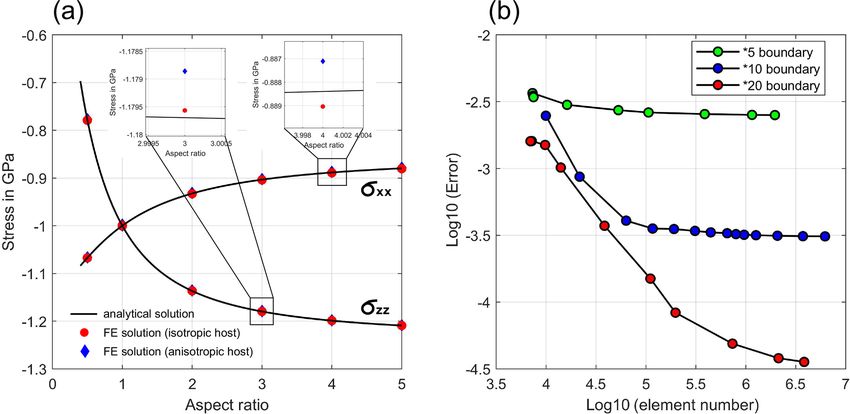
820                                                                  X. Zhong et al.: Analytical solution for residual stress and strain

Figure 1. Schematic diagram showing how to obtain the residual stress and strain of anisotropic inclusion in isotropic host. (a) Inclusion–
host at entrapment conditions. The stress is homogeneous, σtrap , but strains are different, εiincl and εihost . (b) First, relax the inclusion and
host by −εihost to room P –T conditions. Without elastic interaction, the inclusion has strain εiincl − εihost and stress Cijincl (ε incl − ε host ), and
                                                                                                                                    j        j
thus the system is not in mechanical equilibrium. (c) Elastic interaction occurs to reach equilibrium by adding strain εi to the inclusion (host
                                                  incl (ε incl − ε host + ε ). (d) Equivalent scenario where the inclusion and host are initially
also deforms). The residual inclusion stress is Cij      j        j        j
                                                                     host . (e) Equivalent eigenstrains e∗ are loaded to the inclusion. Without
stress-free at room P –T and they both have isotropic elasticity of Cij                                  i
                                                host e∗ . Eshelby’s method is applied to obtain the final strain state in isotropic inclusion, S e∗ ,
elastic interaction, the inclusion has stress −Cij    j                                                                                         ij j
and stress, Cijhost (S e∗ − e∗ ), where S is the Eshelby tensor (Eshelby, 1957). The equivalent eigenstrain method states that by properly
                      jk k     j           ij
                                                                                                                         host (S e∗ − e∗ ), equals
choosing ei∗ , the relation εi = Sij ej∗ can be satisfied (Mura, 1987, chap. 4). The stress of isotropic inclusion (f), Cij     jk k   j

                                               incl   incl  host        ∗                               ∗
the stress of the anisotropic inclusion (c), Cij εj − εj + Sj k ek (see Eq. 7). By solving for ej , we obtain the residual stress and strain
of anisotropic inclusion in isotropic host in Eq. (8).

region with an equivalent eigenstrain ei∗ (to differentiate from               ellipsoidal region of otherwise homogeneous elastic space
the previously introduced eigenstrain term εi∗ due to lattice                  can be expressed as follows (Eshelby, 1957; Mura, 1987):
strain mismatch). Without elastic interaction, the inclusion
would experience a stress −Cijhost ej∗ under perfect confine-                    εires = Sij ej∗
                                                                                                                                                   (4)
ment (e.g. a positive eigenstrain (expansion) leads to com-                      σires = Cijhost Sj k ek∗ − ej∗ ,
pressive stress, which is negative). After elastic interaction,
the inclusion strain and stress under mechanical equilibrium                   where Sij is the Eshelby tensor, which gives the one-to-one
due to a constant eigenstrain (eigenstress) load applied to an                 mapping between the equivalent eigenstrain (ej∗ ) and a ho-
                                                                               mogeneous residual strain (εires ) within the inclusion region.

Solid Earth, 12, 817–833, 2021                                                                         https://doi.org/10.5194/se-12-817-2021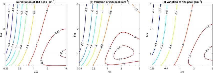
X. Zhong et al.: Analytical solution for residual stress and strain 821
Eshelby’s solution is manifested in this tensor, which is only is represented by a gas or liquid inclusion whose Cijincl is low
a function of the inclusion shape and the Poisson ratio (ν) of compared to the host stiffness; thus, this dimensionless ma-
the isotropic host. For a spherical inclusion, Sij is symmetric trix Mij approaches zero and the isochoric assumption for
and can be significantly simplified as follows: the gas or liquid inclusion is justified. The Mij matrix can be
readily calculated by using the published elastic stiffness ten-
7−5ν
S11 = S22 = S33 = 15(1−ν) sor at room P –T conditions (e.g. Bass, 1995). A MATLAB
5ν−1 script is given in the Supplement to perform this task (details
S12 = S23 = S13 = 15(1−ν) (5)
S44 = S55 = S66 = 4−5ν for using the code can be found in Appendix A–C)
15(1−ν) .
All the other components are zero. For general ellipsoidal 2.3 Back-calculating eigenstrain terms based on
inclusions, the Sij tensor is given in Appendix A–C and a residual inclusion strain
MATLAB script for calculating the Sij tensor is provided in
The wavenumber shifts of Raman peaks are induced by lat-
the Supplement (see Appendix A–C for more details about
tice strain. By measuring wavenumber shift of the inclusion
using the script).
in a thin section, it is possible to recover the residual strain
Following the equivalent eigenstrain method (Mura, 1987,
preserved within the inclusion (Angel et al., 2019; Murri et
chap. 4), one may appropriately choose the equivalent eigen-
al., 2018). This can be done by using the Grüneisen tensor.
strain ej∗ to let Sij ej∗ in Eq. (4) equal the strain εi in Eq. (3)
Therefore, εires can be obtained with, e.g. the least-squares
that drives the pre-strained anisotropic inclusion into me-
fitting method (Murri et al., 2018) and the residual stress can
chanical equilibrium with stress-free isotropic host; i.e. we
be readily expressed as σires = Cijincl εjres .
have
By inverting the right-hand matrix in Eq. (8), the eigen-
εi = Sij ej∗ . (6) strain terms can be expressed as a function of residual strain
εires :
By doing so, the stresses in the original anisotropic hetero- −1
−1
geneity and the equivalent isotropic inclusion will be equal. ε∗i = I − I − S −1 Chost Cincl εres (10)
k .
This is because the host is stressed (and strained) by the same ik
amount following Eq. (6), which leads to the same inclusion
For tetragonal or hexagonal minerals, e.g. zircon, rutile,
stress because the traction is matched between inclusion and
and apatite, the stiffness tensor comprises six independent
host. By replacing the strain εi = Sij ej∗ into σires in Eq. (3) incl , C incl , C incl , C incl , C incl , and C incl . For
components: C11
and equating the stresses σires in Eq. (3) with Eq. (4), we ob- 12 13 33 44 66
trigonal symmetry, such as in the case of α-quartz, another
tain the following relation: incl = −C incl is also present. For
independent component C14 24
all these mineral inclusions and for axially symmetric resid-
σires = Cijincl εjincl − εjhost + Sj k ek∗ = Cijhost Sj k ek∗ − ej∗ . (7)
ual strains, εi∗ can be significantly simplified as follows (εx∗ =
εy∗ 6 = εz∗ ):
The equivalent eigenstrain ek∗ can be solved from this
equation. By substituting the obtained ek∗ back into Eq. (7), 5(1−ν)
h incl incl
incl
i
εx∗ = εxres + 2(7−5ν) C 11 + C 12 εxres + C 13 εzres
we may concisely express the final result for the residual incl
3−5ν incl
strain and stress of the anisotropic inclusion embedded in − 4(7−5ν) 2C 13 εxres + C 33 εzres
isotropic, infinite host: h incl incl
incl
i (11)
3−5ν
εz∗ = εzres − 2(7−5ν) C 11 + C 12 εxres + C 13 εzres
εres
∗ incl
incl
i = Iij − Mij ε j
13−15ν
(8) + 4(7−5ν) 2C 13 εxres + C 33 εzres ,
σ res incl
i = Cik Ikj − Mkj ε j ,
∗
incl
where C ij = Cijincl /G is the dimensionless inclusion stiff-
where Iij is the identity matrix. The dimensionless matrix
ness tensor scaled by the host shear modulus. Interestingly,
Mkj can be expressed as follows: incl 6 = 0), the stiffness ten-
for trigonal α-quartz inclusions (C14
h i−1 incl
sor component C14 is not present in the expression given
Mij = Cincl − Chost I − S −1 Cincl
kj . (9) by Eq. (11). In fact, the terms in the brackets are simply the
ik
residual stress components:
The dimensionless matrix Mij depends on the elastic stiff-
5(1−ν) 3−5ν
ness properties of the inclusion and the host as well as the εx∗ = εxres + 2G(7−5ν) σxres − 4G(7−5ν) σzres
aspect ratio of the inclusion manifested by the Eshelby ten- 3−5ν 13−15ν . (12)
εz∗ = εzres − 2G(7−5ν) σxres + 4G(7−5ν) σzres
sor. The components of this matrix are close to zero for
a stiff host or a soft inclusion (no elastic relaxation; thus, By substituting the stiffness tensor components and the
σires → Cijincl εj∗ ), and it approaches the identity matrix for an measured residual strains, the eigenstrains can be directly
infinitely soft host (in this case, σires → 0). An extreme case calculated. The equation above thus allows for the estimation
https://doi.org/10.5194/se-12-817-2021 Solid Earth, 12, 817–833, 2021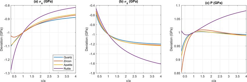
822                                                          X. Zhong et al.: Analytical solution for residual stress and strain

of the entrapment (hydrostatic or non-hydrostatic) stress (or       0.001 GPa. This suggests that it is not necessary in practice to
strain) conditions by knowing the residual stress and strain        consider the anisotropy of garnet host. This has been also re-
conditions of the inclusion.                                        ported in, e.g. Mazzucchelli et al. (2019). It was suggested
                                                                    that the elastic anisotropy of cubic garnet has no signifi-
                                                                    cant impact on the result of elastic barometry. Thus, effective
3   Cross-validation against a finite-element solution              isotropic elastic properties of garnets may be used to model
                                                                    the inclusion–host elastic interaction.
We have validated our implementation of the proposed an-
alytical framework against independent finite-element (FE)
solutions. A self-written 3D FE code is used to validate the        4     Model applications
presented analytical solution (Dabrowski et al., 2008; Zhong
                                                                    4.1    Effect of inclusion aspect ratio on residual stresses
et al., 2018). For validation purposes, we used spheroidal
quartz inclusions in an almandine garnet host. Adaptive             In Eq. (8), the aspect ratio of the inclusion only affects the
tetrahedral computational meshes, with the highest resolu-          Eshelby tensor. Here, we choose some common inclusions
tion within and around the inclusion, are generated with            in metamorphic garnets, including quartz, apatite, zircon, and
Tetgen software (Si, 2015). The anisotropic elastic proper-         rutile, as examples to test the effect of inclusion aspect ratio
ties of quartz inclusion at room T are based on Heyliger            on residual stresses. The data sources of elastic stiffness ten-
et al. (2003). The host garnet elasticity is first treated as       sors of the studied minerals are listed in the caption of Fig. 3.
isotropic based on Jiang et al. (2004). The model length            Here, we first focus on spheroidal inclusions and let the crys-
is set as 10 times (denoted as ×10 below) the inclusion’s           tallographic c axis coincide with the geometrical z axis of the
diameter (for the spheroidal inclusion case, the model do-          inclusion. The inclusion aspect ratio is controlled by varying
main is a box where the side lengths are proportional to the        the lengths of the principal z and x (y) axes, and it is denoted
corresponding axis lengths of the inclusion). For the model         by the c/a ratio for simplicity in the following text (note it
validation, we adjust the eigenstrain term to generate pre-         this is not the ratio of the lattice parameters c and a).
cisely 1 GPa compressive residual stress for the spherical             To isolate the effect of the inclusion aspect ratio, the eigen-
inclusion in the infinite garnet host. This is done by let-         strains for various inclusion minerals are all set to create
       res = σ res = σ res = −1 GPa hydrostatically and substi-
ting σxx       yy     zz                                            1 GPa compressive hydrostatic residual stress for the refer-
tuting σires into Eq. (8) to back-calculate the eigenstrain εj∗ .   ence spherical inclusion embedded in an isotropic, infinite
Following this, the spheroidal inclusion is loaded by the cal-      garnet host, which is the same approach as in the previ-
culated eigenstrain εj∗ in the FE code, and the residual stress     ous “cross-validation” section. Therefore, the stress varia-
is compared to results obtained by the presented analytical         tions shown in Fig. 3 only represent the mechanical effect
solution. The choice of eigenstrains (either loading the in-        due purely to varying the geometrical aspect ratio c/a, and
clusion to 1 GPa pressure or any other residual stress value)       they allow direct comparison among different common min-
is not influential for validation purposes, as long as both the     eral inclusions in metamorphic garnets.
analytical and FE methods take the same eigenstrains. This             Among all the tested minerals, the residual stress in quartz
and other successful and more general tests with arbitrary as-      inclusions is the least sensitive to variations in aspect ratio.
pect ratios and eigenstrains have been performed but are not        For prolate quartz inclusion (c/a>1), the change of σxres due
reported here.                                                      to shape variation is within 0.1 GPa and the change of σzres
   In Fig. 2a, the numerically and analytically obtained resid-     is within 0.2 GPa. The effects of varying the aspect ratio of
ual stresses are plotted together as a function of the aspect       prolate zircon and apatite inclusions are similar, with varia-
ratio of the tested spheroidal inclusions. In Fig. 2b, the dif-     tion of σxres from the reference spherical case reaching up to
ference is plotted as a function of element count and bound-        ca. 0.12 GPa and σzres up to ca. 0.2 GPa.
ary distance (×5, ×10, and ×20). It is clearly shown that the          The residual stress in rutile is the most sensitive to aspect
two sets of solutions converge with increasing the number           ratio variations. With increasing c/a ratio from 1, σxres in pro-
of mesh elements and the computational box size. The suc-           late rutile inclusions increases up to ca. 0.2 GPa, and σzres
cess of this convergence test validates the correctness of our      decreases by ca. 0.6 GPa. This is relevant for practical mea-
presented analytical model (also FE code) for an anisotropic        surement as rutile often forms needle-shaped crystals.
ellipsoidal inclusion entrapped in an isotropic space.                 The pressure (negative mean stress) is significantly less
   In addition, we have also tested the effect of applying          sensitive to inclusion aspect ratio variations. For prolate in-
cubic elastic stiffness tensor of almandine from Jiang et           clusions of quartz, zircon, and apatite, the residual pressure
al. (2004) and compared the residual stress with the re-            differs from the reference level (spherical inclusion shape)
sults obtained for an elastically isotropic garnet (blue dots       by only ca. 0.01 GPa when the aspect ratio c/a is stretched
in Fig. 2a). The difference in residual stresses obtained with      up to 4. For oblate inclusion (c/a
X. Zhong et al.: Analytical solution for residual stress and strain 823
Figure 2. Cross-validation results between a finite-element method and the presented analytical method. (a) Direct comparison of residual
stress components calculated with FE method and analytical method as a function of the aspect ratio of a spheroidal inclusion. (b) The
normalized unsigned difference of the stress between FE method and analytical method as a function of mesh element number and model
domain size. Spherical inclusion is used and boundary distance is set to ×5, ×10, and ×20 the inclusion diameter.
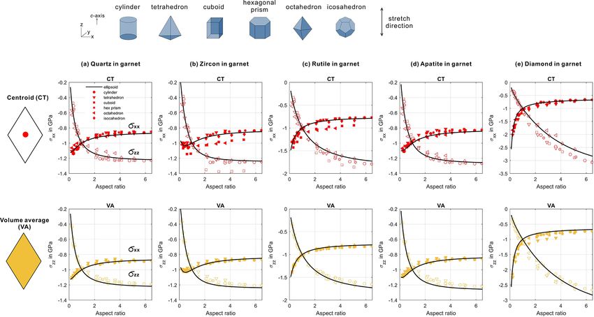
Figure 3. Effect of geometrical aspect ratio of spheroidal inclusion along c and a axes on residual stress (c/a). (a, b) Stresses σxx res and σ res as
zz
a function of the geometrical c/a ratio for quartz, zircon, apatite, and rutile inclusions. To isolate the effects of aspect ratio, the eigenstrain are
res = σ res = −1 GPa for the reference spherical inclusion. Any deviation from −1 GPa is due to shape changes. (c) Pressure
set to produce σxx zz
as a function of the c/a ratio. Here, the crystallographic c axis is aligned parallel to the long axis for prolate inclusions and the short axis for
oblate inclusions. The quartz elastic stiffness tensor is from Heyliger et al. (2003), zircon and diamond are from Bass (1995), rutile is from
Wachtman et al. (1962), and apatite is from Sha et al. (1994). The isotropic stiffness tensor of the almandine host is from Milani et al. (2015).
The residual stress in mineral inclusions can be easily con- of less than 0.3 cm−1 for the 464 cm−1 Raman peak. This
verted into residual strain, which can be directly translated is in most cases insignificant from the viewpoint of practi-
into Raman shifts (Angel et al., 2019; Murri et al., 2018). The cal Raman measurements. The b/a ratio variations are also
effects of varying the aspect ratio of a quartz inclusion on Ra- shown to be insignificant for the spectral shifts, with changes
man wavenumber shifts (see Fig. 4) are determined using the less than 0.2 cm−1 for the 464 cm−1 peak. For oblate inclu-
calculated residual strain components and the Grüneisen ten- sion, the impact of inclusion shape is shown to be more sig-
sor (Murri et al., 2018). The same model settings are applied, nificant. For the 464 cm−1 peak, the change of wavenum-
with 1 GPa compressive hydrostatic residual stress charac- ber shift can reach 0.8 cm−1 for strongly oblate inclusion
terizing the case of a spherical quartz inclusion. It is shown (c/a = 0.25), and it is ca. 0.3–0.4 cm−1 for less oblate in-
that for prolate inclusions, aspect ratio only introduces mi- clusion (c/a = 0.5).
nor effects on the Raman shifts. For example, varying the Our results show good consistency with the Raman data
c/a ratio between 1 and 5 induces a wavenumber variation reported in Kouketsu et al. (2014), where quartz inclusions
https://doi.org/10.5194/se-12-817-2021 Solid Earth, 12, 817–833, 2021824 X. Zhong et al.: Analytical solution for residual stress and strain Figure 4. The effect of geometrical aspect ratio of ellipsoidal quartz inclusion for c/a axes and b/a axes on Raman wavenumber shift entrapped in garnet host. The contours show the variation of wavenumber shift compared to perfectly spherical quartz inclusion (c/a = 1, b/a = 1). The initial residual inclusion pressure is assumed to be hydrostatic 1 GPa for the reference spherical inclusion. The wavenumber shift variations are due to changing the geometrical aspect ratios of c/a and b/a axes. The Raman shifts are calculated using the residual strain and the Grüneisen tensor in Murri et al. (2018). For c/a>1 the inclusion is prolate, and for c/a
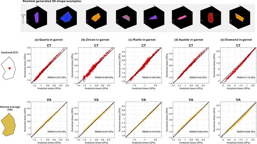
X. Zhong et al.: Analytical solution for residual stress and strain                                                                        825

Figure 5. The effect of varying the crystallographic orientation (c axis) with respect to the geometrical long axis of a prolate spheroidal
quartz inclusion. The contours show the variation of wavenumber shift compared to perfectly spherical quartz inclusion c/a = 1 (in this case
the crystallographic orientation does not matter). The horizontal axis represents the aspect ratio of the spheroidal inclusion, and the vertical
axis shows the angle between the crystallographic c axis and the geometrical long axis. In the plot, c axis is allowed to shift from parallel
to the geometrical long axis to parallel to the geometrical short axis of the spheroidal inclusion. The driving eigenstrain is set to produce a
hydrostatic residual pressure of 1 GPa in the reference spherical inclusion.

ratio, the inclusion shape is stretched in the z axis direction,          ally lower than 0.02–0.03 GPa (ca. 2 %). From CT to VA, a
which is parallel to the crystallographic c axis as shown in              significant improvement on RMSD of a factor of abour 2 is
Fig. 6.                                                                   obtained.
   We study five inclusion minerals: quartz (elastic ten-                    The only exception among the studied minerals is dia-
sor from Heyliger et al., 2003), zircon (Bass, 1995), rutile              mond, where the RMSD is higher than in the case of other
(Wachtman et al., 1962), fluorapatite (Sha et al., 1994), and             inclusions, which are elastically softer. This is consistent
diamond (Bass, 1995). Almandine garnet is taken as the host               with the high “geometrical correction factor” reported for
grain (Milani et al., 2015). For each FE mesh, the size of the            diamond in Mazzucchelli et al. (2018). However, as an im-
computational box is set more than 10 times the inclusion                 provement from Mazzucchelli et al. (2018), where the geo-
size and adaptive mesh is generated with highest mesh reso-               metrical correction factor must be applied for all inclusion
lution within and close to the inclusion. The 10-node tetrahe-            phases to correct the residual stress due to shape effects,
dron elements with quadratic (second-order) shape (interpo-               we have found that the stress variation due to varying inclu-
lation) functions for the displacement field are used. In total,          sion shapes for minerals such as quartz, zircon, apatite, and
there are ca. 2 million elements per model (relative error of             rutile can be satisfactorily approximated by using the pro-
less than 0.0003 based on benchmark results in Fig. 2).                   posed approach of the equivalent ellipsoidal inclusion, with
   The results of numerical simulations are shown in Fig. 6.              RMSD generally lower than 3 %–4 % for most of the stud-
The effective aspect ratio for all different inclusion shapes,            ied inclusion shapes. To achieve this improved and satisfac-
together with the residual stress components, are given in the            tory level of prediction (1) we have used best-fit ellipsoids
Supplement. The residual stress in non-ellipsoidal inclusions             to better approximate inclusion shapes, instead of a crude
based on the FE model is heterogeneous and we monitor the                 measure of the length/width ratio of, e.g. cuboidal or cylin-
stress state (1) at the centroid (CT) point (red dots in Fig. 6)          drical inclusion, and (2) we have not only considered the
and (2) as the volumetric average (VA) within the entire in-              centroid point of the inclusion (which indeed yields a larger
clusion (orange dots)                                                     RMSD) but also the volumetric average (VA) for the residual
   The root-mean-square deviation (RMSD) is calculated by                 stress state sampled during stress measurements, which in-
comparing the residual stress from the finite-element solu-               terestingly provides a significantly better approximation for
tions based on various stress evaluation schemes (CT and                  the residual stress or strain state of the tested mineral inclu-
VA) and analytical models using the best-fitted effective as-             sions. This is practical and useful in Raman measurement
pect ratio (Table 1). It is clearly shown that the VA stresses            because it is possible to perform either (1) multiple-point av-
of quartz, zircon, rutile, and apatite inclusion are remark-              eraging during Raman analysis within the entire inclusion or
ably similar to the analytical results, with an RMSD gener-               (2) defocus the laser beam to take into account a larger vol-

https://doi.org/10.5194/se-12-817-2021                                                                     Solid Earth, 12, 817–833, 2021
826                                                              X. Zhong et al.: Analytical solution for residual stress and strain

Figure 6. Finite-element stress of various inclusion shapes (symbols) compared to the stress of effective spheroidal inclusion based on
an analytical method (black curves). The effective aspect ratio of inclusion shape is calculated based on the fitting method of Chaudhuri
and Samanta (1991) and Li et al. (1999) (see Appendix A–C). The inclusion is loaded with eigenstrain that generates 1 GPa compressive
hydrostatic residual stress for spherical shape. The variation of stress is only caused by the shape change. The c axis coincides with the
stretching direction. The red dots correspond to the stress at the inclusion’s centroid (CT); the orange dots correspond to the volumetric
average (VA) of the entire inclusion. The anisotropic elastic stiffness tensors are listed in the caption of Fig. 3. The root-mean-square
deviation (RMSD) for each inclusion shape and inclusion mineral phase is given in Table 1. The raw FE stress data can be found in the
Supplement.

Table 1. Root-mean-square deviation (RMSD) of the finite-element solution of symmetrically shaped non-ellipsoidal inclusion in Fig. 6
compared to the analytical solution of equivalent spheroidal inclusions. Isotropic almandine garnet is used as a host. For each inclusion
mineral and inclusion shape, the aspect ratio varies from 0.2 to 5. The effective aspect ratio is calculated for each shape and used for the
analytical solution to obtain the residual stress state. The inclusion is loaded by eigenstrain that creates 1 GPa hydrostatic residual pressure
for spherical inclusion in an infinite host. Thus, any stress variation can only be caused by shape change. The calculated stress data for each
individual FE run is given in Supplement data. Stress is obtained for (1) the centroid point (CT) and (2) volumetric average (VA) of the entire
inclusion (see Fig. 6 for illustration). The RMSD is calculated by comparing the FE results and analytical results based on the best-fitted
effective ellipsoid. The unit used for RMSD is GPa. The elasticity of the inclusion mineral given in the caption of Fig. 6.

          Shape           Cylinder         Tetrahedron          Cuboid        Hexagonal prism        Octahedron        Icosahedron
          Location       CT       VA       CT        VA       CT       VA       CT          VA        CT       VA       CT       VA
          Quartz       0.041    0.021    0.034     0.044    0.042    0.026    0.038       0.021     0.055    0.022    0.011    0.005
          Zircon       0.045    0.023    0.042     0.048    0.112    0.028    0.047       0.024     0.084    0.017    0.028    0.006
          Rutile       0.063    0.039    0.049     0.029    0.158    0.039    0.065       0.039     0.127    0.026    0.034    0.003
          Apatite      0.047    0.029    0.052     0.057    0.049    0.035    0.045       0.029     0.062    0.024    0.014    0.007
          Diamond      0.136    0.071    0.191     0.255    0.171    0.095    0.136       0.081     0.079    0.125    0.022    0.027

ume for the inclusion strain heterogeneity. For tiny inclusions           eraged stress within the inclusion, rather than centroid point
(size of ca. 1–3 µm) and for a typical in-plane laser beam di-            measurements, may provide a closer match compared to the
ameter of ca. 1–2 µm, the stress and strain averaging is, in              stress predicted based on the presented analytical solution de-
fact, implicitly performed during measurements. Based on                  veloped for the best-fitted ellipsoid. This effect becomes sta-
FE analysis, it is clearly shown that the volumetrically av-              tistically more significant when the faceted inclusion shape

Solid Earth, 12, 817–833, 2021                                                                    https://doi.org/10.5194/se-12-817-2021
X. Zhong et al.: Analytical solution for residual stress and strain 827
and crystallographic orientation are independent, as demon- ment of the orange dots and 1-to-1 ratio line in the middle
strated in the next section. and bottom panels of Fig. 7).
Thus, the volumetric average of the residual stress within
4.4 Irregularly faceted shapes and random the inclusion provides a sufficiently reliable match between
crystallographic orientation the exact results for irregularly shaped inclusions and the ap-
proximate predictions based on the analytical solution. This
In nature, the shape of mineral inclusions is not necessar- shows that it is possible to approximate the stress and strain
ily as highly symmetric as presented in the previous section, state of the inclusion using an effective ellipsoid shape for
and the crystallographic orientation can be generally random the tested inclusions including quartz, zircon, rutile, and ap-
with respect to the principal geometric axes of the inclu- atite. Only diamond has a notably higher level of RMSD, ex-
sion. Here, a MATLAB script is used to generate completely hibiting a systematic discrepancy between the exact numer-
random 3D inclusion shapes by prescribing random vertices ical and approximate analytical results. This indicates that
(non-coplanar 5 to 24 vertices) and connecting them to form using the proposed equivalent analytical model for diamond
a closed 3D shape. Delaunay triangulation is used to form inclusion may lead to a potential overestimation of the resid-
3D volumes enclosed by the triangular faces. Tetgen soft- ual stress by ca. 0.07 GPa (7 %). However, this RMSD may
ware is again used to generate unstructured tetrahedron com- still be acceptable as a crude estimate or may serve as an
putational meshes fitted to the inclusion surface. The effec- upper limit for elastic thermobarometry.
tive aspect ratio (geometrical longest to shortest axis of the
best-fitted effective ellipsoid) is controlled to be within 6. In
total, we have generated ca. 500 random 3D inclusion shapes 5 Non-linear elasticity at room T
and performed a finite-element simulation for the previously
studied set of anisotropic inclusion minerals (quartz, zircon, The presented model builds on a linear elastic constitutive
rutile, apatite, and diamond) to calculate the elastic stress law at room temperature, i.e. σires = Cijincl εjres . This assump-
field. The generated random shapes are plotted in the Sup- tion is appropriate when the residual stresses and strains of
plement (see the .gif animation that illustrates 100 selected the inclusion are low, and thus the application of a con-
examples of 3D inclusion shapes). We further allow the crys- stant anisotropic stiffness tensor Cijincl determined at room
tallographic c axis to be pointing along an orientation that is P –T conditions introduces no significant errors. For highly
randomly chosen as parallel to either the longest, intermedi- stressed mineral inclusions, e.g. inclusions in diamond host
ate, or shortest geometrical axis (best-fitted using the method from mantle xenoliths where the residual inclusion pressure
of Chaudhuri and Samanta, 1991). The FE results are com- may reach several GPa, this approximation may lead to non-
pared to the analytical results based on the effective ellip- negligible deviations. To eliminate such error, the stiffness
soidal inclusion with the same crystallographic orientation. tensor Cijincl needs to be treated as a function of either non-
This Monte Carlo type FE simulation allows us to investi- hydrostatic stresses or anisotropic strains, i.e. Cijincl (σires ) or
gate how much stress deviation can be generated for irregu- Cijincl (εires ). In experimental studies, Cijincl is often described
larly faceted inclusion shapes with random crystallographic as a function of hydrostatic pressure, e.g. Bass (1995). It is
orientation and how accurate the analytical approach based beyond the scope of this paper to develop a method of fit-
on the best-fitted ellipsoid is to describe the residual stress ting Cijincl with respect to the individual stress tensor compo-
state in an irregularly shaped inclusion, depending on the nents. If the stiffness tensor Cijincl can be parameterized by
stress-sampling scheme (CT and VA). The results are plot- σires or simply as a function of pressure as a first-order ap-
ted in Fig. 7 (raw data of FE simulations can be found in proximation, the residual stresses and strains are readily cal-
Supplement). culated by iterating Eq. (8), while updating the Cijincl tensor
For the centroid point (CT), quartz inclusions have the using the calculated inclusion stress or strain during the iter-
lowest RMSD (ca. 0.03 GPa) for all three normal stress com- ation loop. Thus, the developed analytical method based on
ponents and diamond inclusions have the highest RMSD the Eshelby’s solution can be extended to the case of a non-
(ca. 0.11 GPa). In general, CT stress shows a systematically linear inclusion phase as long as Cijincl can be parameterized
higher RMSD than volumetrically averaged (VA) stresses. in terms of stress or strain components or their invariants.
When the stress within the inclusion is volumetrically av-
eraged, the RMSD dramatically drops to a nearly perfect
match between the FE results for irregularly faceted inclu- 6 Concluding remarks and petrological implications
sion and the analytical prediction based on the best-fitted
ellipsoid. The RMSD of volumetrically averaged residual In this study, we use the classical Eshelby solution combined
stresses (VA) of quartz, zircon, rutile, and apatite are all with the equivalent eigenstrain method to calculate the resid-
lower than ca. 0.02 GPa (2 %), and it shows no obvious de- ual strain and stress in an anisotropic, ellipsoidal mineral in-
pendence on the effective aspect ratio even for the extremely clusion embedded in an elastically isotropic host. The resid-
elongated or flattened inclusions (see the near-perfect align- ual stresses can be expressed by a linear operator (Eq. 8) act-
https://doi.org/10.5194/se-12-817-2021 Solid Earth, 12, 817–833, 2021828 X. Zhong et al.: Analytical solution for residual stress and strain Figure 7. The 500 randomly generated inclusion shapes (top panel for examples) calculated with the finite-element method (vertical axis) and analytical method (horizontal axis). All three normal stress components are plotted together in each diagram. The crystallographic c axis orientation is randomly chosen along one of the geometrical principal axes. The red and orange dots show the comparison of FE (numerical) results and analytical results for the normal stress components, respectively. Each dot represents a normal stress component calculated for one randomly generated inclusion shape. The red dots show the stress evaluated at the centroid point (CT); the orange dots show the volumetrically averaged (VA) stress within the inclusion. The raw data can be found in the Supplement and the generated 3D random shape can be viewed in the accompanying .gif file. ing on the eigenstrain. The linear operator depends on the the crystallographic c axis orientation when studying highly anisotropic elastic stiffness tensor of the inclusion evaluated stretched or flattened quartz inclusions. As long as the c axis at room P –T conditions, the shape of the inclusion, and the is sub-parallel to the geometrical long axis, the additional shear modulus and Poisson ratio of the host. The studied me- wavenumber shifts due to the inclusion aspect ratio are mi- chanical problem is loaded by an eigenstrain term, which is nor. given by the difference between the lattice strains of the in- Our proposed analytical procedures to model residual in- clusion and host at the P –T conditions of entrapment. clusion stress and strain state do not require pre-FE simula- The effect of inclusion aspect ratio on the inclusion resid- tion to obtain the six-by-six “relaxation tensor” as proposed ual stress and strain has been investigated quantitatively. The by Mazzucchelli et al. (2019). For application purposes, as residual stress in quartz inclusions exhibits the least sen- long as the lattice strains of inclusion (εiincl ) and host (εihost ) sitivity to aspect ratio changes, and rutile shows the most at high P –T conditions are available, it is possible to cal- pronounced variation. The popularly used quartz-in-garnet culate the eigenstrain term by subtracting them following system is studied in more detail. For prolate quartz inclu- Eq. (2). Given the driving eigenstrain, the residual strain and sions, the residual stress variations caused by varying inclu- stress preserved within an anisotropic, ellipsoidal inclusion sion shape are shown to be insignificant when the crystal- in isotropic host can be easily calculated using Eq. (8). The lographic c axis is subparallel to the geometrical long axis. proposed procedure can be inversely applied to retrieve the The Raman wavenumber variation is less than 0.4 cm−1 for residual strain and stress of any natural mineral inclusions the 464 cm−1 peak even for highly elongated inclusions with embedded in elastically isotropic hosts, such as garnets. an aspect ratio of 5. For oblate quartz inclusions with an as- The presented model is only exact for perfectly ellip- pect ratio of ca. 0.5, the additional wavenumber shift may soidal inclusions. In nature, inclusions often possess differ- reach ca. 0.8 cm−1 . Therefore, it is useful in practice, al- ent shapes with facets and edges. Finite-element simulations though potentially technically difficult, to have an estimate of on various faceted inclusion shapes showed that the resid- Solid Earth, 12, 817–833, 2021 https://doi.org/10.5194/se-12-817-2021
X. Zhong et al.: Analytical solution for residual stress and strain                             829

ual stress is modified to a different degree compared to the
simple ellipsoidal inclusion case, depending on the relative
elastic properties between the inclusion and the host grain.
However, the proposed approach of using the analytical re-
sult for the best-fitted effective ellipsoids yields remarkably
good approximation for all the tested inclusion shapes, in-
cluding highly irregular shapes. The RMSD comparing the
FE numerical solution for faceted inclusion and the analytical
solution based on a effective best-fitted ellipsoid is typically
less than 2 % for quartz, zircon, apatite, and rutile inclusions.
The only exception are the elastically stiff diamond inclu-
sions, where the RMSD reaches 7 %. This finding expands
the applicability of the analytical framework to arbitrarily
shaped inclusions, whose elastic stiffness is not significantly
higher than host (such as quartz, rutile, zircon and apatite).
One important petrological implication is that it is possible to
take the volumetrically averaged stress and strain within the
inclusion and use it as a proxy to represent the residual stress
and strain state of the inclusion. Then the proposed analytical
framework may be used to recover the entrapment condition
by back-calculating the eigenstrain using the volumetrically
averaged residual stress and strain and the effective ellipsoid
aspect ratio of the inclusion (Eq. 8). In fact, averaging the
stress and strain within a certain volume is implicitly done
in practical Raman measurement, e.g. for a tiny micrometre-
sized inclusion with a laser beam size typically exceeding
1 µm.

https://doi.org/10.5194/se-12-817-2021                                Solid Earth, 12, 817–833, 2021
830 X. Zhong et al.: Analytical solution for residual stress and strain
Appendix A: Calculating lattice strain under finite Lagrangian strain tensor reported in MATLAB com-
entrapment conditions mend window. The results are numerically the same com-
pared to the available computer programmes such as the
When the inclusion and host are crystalized at entrapment “STRAIN” programme, which can be found at https://www.
conditions, they are considered to be stressed and strained by cryst.ehu.es/cryst/strain.html (last access: 8 April 2021), or
taking the room P –T condition as the reference state. There- the “Win_Strain” programme.
fore, it is possible to calculate their strain state using lattice
parameters a, b, and c relative to the reference state a0 , b0 ,
c0 . For cubic, tetragonal, and orthorhombic symmetry sys- Appendix B: Calculating Eshelby’s tensor
tems (or hexagonal and trigonal minerals with symmetry be-
ing imposed), the lattice strains can be easily expressed fol- The components of Eshelby’s tensor Sij are expressed as
lowing Eq. (1). For triclinic and monoclinic symmetry sys- functions of the inclusion’s principal axes lengths and the
tems, the basis vectors of unit cell are not all parallel to the Poisson ratio of the isotropic host ν (Mura, 1987). A MAT-
Cartesian coordinates x, y, and z. To obtain the lattice strain, LAB script is provided to calculate Eshelby’s tensor (for
we need use the unit cell parameters before and after the de- more detail, see the Supplement).
formation and transform them into strains in the x, y, and 3a12 1−2ν
S11 = 8π(1−ν) I11 + 8π(1−ν) I1
z directions. We follow the method from Ohashi and Burn- 3a22 1−2ν
ham (1973) to calculate the strain components based on the S22 = 8π(1−ν) I22 + 8π(1−ν) I2
3a3 2
lattice parameters. Here, a short description on the involved S33 = 1−2ν
8π(1−ν) I11 + 8π(1−ν) I3
equations is given and detailed can be found the in the ap- a22
1−2ν
pendix to Ohashi and Burnham (1973). This transformation S12 = 8π(1−ν) I12 − 8π(1−ν) I1
considers the crystallographic c axis parallel to the Cartesian a12 1−2ν
S21 = 8π(1−ν) I12 − 8π(1−ν) I2
z axis and crystallographic a* axis parallel to the Cartesian a32
1−2ν
x axis. S13 = 8π(1−ν) I13 − 8π(1−ν) I1
a12 (B1)
The matrix Q0 that relates the basis vectors of undeformed 1−2ν
S31 = 8π(1−ν) I13 − 8π(1−ν) I3
crystallographic a0 , b0 , and c0 axes at reference room P –T a22
1−2ν
conditions to Cartesian coordinates is as follows: S23 = 8π(1−ν) I23 − 8π(1−ν) I2
a32
1−2ν
a0 p0 a0 (cos(γ0 )−cos(α0 ) cos(β0 ))
S32 = 8π(1−ν) I23 − 8π(1−ν) I3
sin(α0 ) sin(α0 ) a0 cos(β0 )
Q0 = a22 −a32 1−2ν
0 b0 sin(α0 ) b0 cos(α0 ) S44 = 16π(1−ν) I23 + 16π(1−ν) (I2 + I3 )
0 0 c0 2
a1 −a3 2
h
(A1) 1−2ν
p0 = 1 − cos2 (α0 ) − cos2 (β0 ) − cos2 (γ0 ) S55 = 16π(1−ν) I13 + 16π(1−ν) (I1 + I3 )
2
a1 −a2 2
1−2ν
i1/2 S66 = 16π(1−ν) I12 + 16π(1−ν) (I1 + I2 )
+2 cos (α0 ) cos (β0 ) cos (γ0 ) ,
Here a1 , a2 , and a3 are the lengths of three principal axes
Obtaining a similar transformation matrix relating the de- of the inclusions, and they follow the order of a1 > a2 > a3 .
formed crystallographic axes at entrapment conditions to In case this order needs to be changed, a simple 90◦ rotation
Cartesian coordinates can be easily done by replacing a0 , can be executed on Sij . The provided code in the Supplement
b0 c0 , α0 , β0 , and γ0 measured at reference P –T state with automatically performs such a rotation to adjust the axes into
a, b, c, α, β, and γ measured at the entrapment conditions the correct order. The required tensors Ii and Iij are evalu-
from Eq. (A1). This transformation matrix is denoted as Q1 . ated as follows.
We then calculate the displacement gradient tensor E as fol- I1 = 4πa1 a2 a3
[F (θ, k) − E (θ, k)]
1/2
a12 −a22 a12 −a32
lows: 1/2
4πa1 a2 a3 a2 a12 −a32
E = Q−1 I3 = − E (θ, k)
0 Q1 − I, (A2) a22 −a3 a1 −a3
2 2 2 1/2 a1 a3
I2 = 4π − I1 − I3
where I is the identity matrix. Without considering the anti- I12 = I22 −I12
symmetric rotation tensor, the infinitesimal Lagrangian strain a1 −a2
I3 −I1
tensor can be expressed as follows: I13 =
a12 −a32
I3 −I2 (B2)
I23 =
ε = (E 0 + E)/2. (A3) a22−a32
1 4π
A MATLAB code is provided to perform this calcula- I11 = − I12 − I13
3 a12
tion (Calculate_Strain.m). The input values are the 1 4π
reference lattice parameters measured at room P –T con- I22 = − I12 − I23
3 a22
ditions and the deformed lattice parameters at the entrap- 1 4π
ment conditions. The outputs are both the infinitesimal and I33 = − I13 − I23
3 a32
Solid Earth, 12, 817–833, 2021 https://doi.org/10.5194/se-12-817-2021You can also read


