Spiciness theory revisited, with new views on neutral density, orthogonality, and passiveness - Ocean Science
←
→
Page content transcription
If your browser does not render page correctly, please read the page content below
Ocean Sci., 17, 203–219, 2021
https://doi.org/10.5194/os-17-203-2021
© Author(s) 2021. This work is distributed under
the Creative Commons Attribution 4.0 License.

Spiciness theory revisited, with new views on neutral density,
orthogonality, and passiveness
Rémi Tailleux
Dept. of Meteorology, University of Reading, Earley Gate, RG6 6ET Reading, United Kingdom

Correspondence: Rémi Tailleux (r.g.j.tailleux@reading.ac.uk)

Received: 26 April 2020 – Discussion started: 20 May 2020
Revised: 8 December 2020 – Accepted: 9 December 2020 – Published: 28 January 2021

Abstract. This paper clarifies the theoretical basis for con-         1   Introduction
structing spiciness variables optimal for characterising ocean
water masses. Three essential ingredients are identified: (1) a       As is well known, three independent variables are needed to
material density variable γ that is as neutral as feasible, (2) a     fully characterise the thermodynamic state of a fluid parcel in
material state function ξ independent of γ but otherwise ar-          the standard approximation of seawater as a binary fluid. The
bitrary, and (3) an empirically determined reference function         standard description usually relies on the use of a tempera-
ξr (γ ) of γ representing the imagined behaviour of ξ in a            ture variable (such as potential temperature θ , in situ temper-
notional spiceless ocean. Ingredient (1) is required because          ature T , or Conservative Temperature 2), a salinity variable
contrary to what is often assumed, it is not the properties im-       (such as reference composition salinity S or Absolute Salin-
posed on ξ (such as orthogonality) that determine its dynam-          ity SA ), and pressure p. In contrast, theoretical descriptions
ical inertness but the degree of neutrality of γ . The first key      of oceanic motions only require the use of two “active” vari-
result is that it is the anomaly ξ 0 = ξ − ξr (γ ), rather than ξ ,   ables, namely in situ density ρ and pressure. The implication
that is the variable most suited for characterising ocean wa-         is that S and θ can be regarded as being made of an active
ter masses, as originally proposed by McDougall and Giles             part contributing to density and a passive part associated with
(1987). The second key result is that oceanic sections of nor-        density-compensated variations in θ and S – usually termed
malised ξ 0 appear to be relatively insensitive to the choice of      “spiciness” anomalies – which behaves as a passive tracer.
ξ , as first suggested by Jackett and McDougall (1985), based         Physically, such an idea is empirically supported by numer-
on the comparison of very different choices of ξ . It is also         ical simulation results showing that the turbulence spectra
argued that the orthogonality of ∇ξ 0 to ∇γ in physical space         of density-compensated thermohaline variance is generally
is more germane to spiciness theory than orthogonality in             significantly different from that contributing to the density
thermohaline space, although how to use it to constrain the           (Smith and Ferrari, 2009).
choices of ξ and ξr (γ ) remains to be fully elucidated. The re-         Although behaving predominantly as passive tracers,
sults are important for they unify the various ways in which          density-compensated anomalies may occasionally “activate”
spiciness has been defined and used in the literature. They           and couple with density and ocean dynamics. This may
also provide a rigorous theoretical basis justifying the pursuit      happen, for instance, when isopycnal mixing of θ and S
of a globally defined material density variable maximising            leads to cabbeling and densification, which may create avail-
neutrality. To illustrate the latter point, this paper proposes a     able potential energy (Butler et al., 2013); when density-
new implementation of the author’s recently developed ther-           compensated temperature anomalies propagate over long
modynamic neutral density and explains how to adapt exist-            distances to de-compensate upon reaching the ocean sur-
ing definitions of spiciness and spicity to work with it.             face, thus modulating air–sea interactions (Lazar et al.,
                                                                      2001); when density-compensated salinity anomalies prop-
                                                                      agate from the equatorial regions to the regions of deepwa-
                                                                      ter formation, thus possibly modulating the strength of the
                                                                      thermohaline circulation (Laurian et al., 2006, 2009); and/or

Published by Copernicus Publications on behalf of the European Geosciences Union.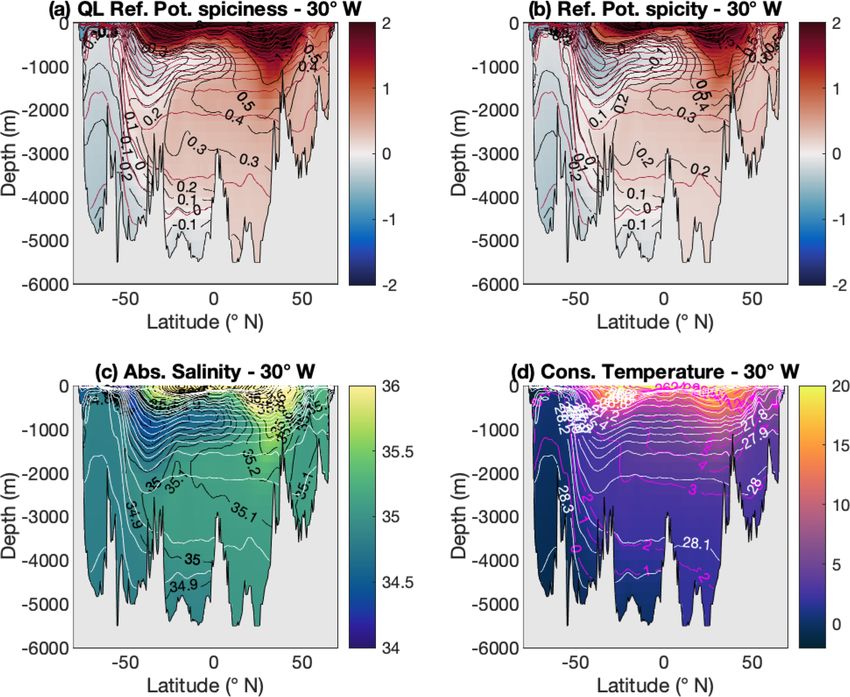
204                                                                                        R. Tailleux: Spiciness theory revisited

when isopycnal stirring of density-compensated θ/S anoma-            following. “Secondly, it is readily apparent that the per-
lies releases available potential energy associated with ther-       pendicular property itself has no inherent physical mean-
mobaric instability (Ingersoll, 2005; Tailleux, 2016a). For          ing since a simple rescaling of either the potential temper-
these reasons, the mechanisms responsible for the formation,         ature θ or the salinity axis S destroys the perpendicular prop-
propagation, and decay of spiciness anomalies have received          erty”. The Jackett and McDougall (1985) remarks are impor-
much attention, with a key research aim being to understand          tant for at least two reasons: (1) first, for suggesting that it
their impacts on the climate system; e.g. Schneider (2000),          is really the isopycnal anomaly ξ 0 = ξ − ξr (γ ) defined rela-
Yeager and Large (2004), Luo et al. (2005), Tailleux et al.          tive to some reference function of density ξr (γ ) that is dy-
(2005), and Zika et al. (2020).                                      namically passive and therefore the quantity truly measur-
   From a dynamical viewpoint, in situ density ρ is the most         ing spiciness. This was further supported by McDougall and
relevant density variable for defining density-compensated           Giles (1987) subsequently arguing that it is such an anomaly
θ/S anomalies, but its strong pressure dependence makes              that represents the most appropriate approach for character-
the associated isopycnal surfaces strongly time-dependent            ising water mass intrusions. Note here that if one defines
and therefore impractical to use. This is why in practice            reference salinity and temperature profiles Sr (γ ) and θr (γ )
oceanographers prefer to work with isopycnal surfaces de-            such that γ (Sr (γ0 ), θr (γ0 )) = γ0 , using a Taylor series ex-
fined by means of a purely material density-like variable            pansion shows that S 0 = S − Sr (γ ) and θ 0 = θ − θr (γ ) are γ -
γ = γ (S, θ ) unaffected by pressure variations. Since density-      compensated at leading order, i.e. they satisfy γS S 0 + γθ θ 0 ≈
compensated θ/S anomalies are truly passive only if defined          0, and hence approximately passive. (2) The second reason
in terms of in situ density, γ needs to be able to mimic the         is for establishing that the imposition of any form of orthog-
dynamical properties of in situ density as much as feasible.         onality between ξ and γ is even less meaningful than previ-
As discussed by Eden and Willebrand (1999), this amounts             ously realised, since even if ξ is constructed to be orthogonal
to imposing that γ be constructed to be as neutral as feasible.      to γ in some sense, this orthogonality is lost by the anomaly
Because of the thermobaric non-linearity of the equation of          ξ 0 = ξ − ξr (γ ).
state, it is well known that exact neutrality cannot be achieved         If one accepts that it is the spiciness anomaly ξ 0 = ξ −
by any material variable. As a result, investigators have re-        ξr (γ ) rather than the spiciness as a state function (ξ ) that is
sorted to using either neutral surfaces (McDougall and Giles,        the most appropriate measure of water mass contrasts, as ar-
1987) or potential density referenced to a pressure close to         gued by Jackett and McDougall (1985) and McDougall and
the range of pressures of interest (Jackett and McDougall,           Giles (1987), the central questions that the theory of spici-
1985; Huang, 2011; McDougall and Krzysik, 2015; Huang                ness needs to address become the following.
et al., 2018). In this paper, I propose instead using a new im-
plementation of the Tailleux (2016b) thermodynamic neutral             1. Are there any special benefits associated with one par-
density variable γ T , which is currently the most neutral ma-            ticular choice of spiciness as a state function (ξ ) over
terial density-like variable available. The resulting new vari-           another, and if so, what are the relevant physical argu-
                           T
able is referred to as γanalytic  in the following, and details of        ments that should be invoked to establish the superiority
its construction and implementation are given in Sect. 2.                 of any given particular choice of ξ ?
   Once a choice for γ has been made, a second material vari-
                                                                       2. How should γ and the reference function ξr (γ ) be con-
able ξ = ξ(S, θ ) is required to fully characterise the thermo-
                                                                          structed and justified?
dynamic properties of a fluid parcel. From a mathematical
viewpoint, the only real constraint on ξ is that the transfor-         3. While any ξ independent of γ can be used to meaning-
mation (S, θ ) → (γ , ξ ) defines a continuously differentiable           fully compare the spiciness of two different water sam-
one-to-one mapping (that is, an isomorphism) so that (S, θ )              ples lying on the same isopycnal surface γ = constant,
properties can be recovered from the knowledge of (γ , ξ ).               it is generally assumed that it is not possible to mean-
For this, it is sufficient that the Jacobian J = ∂(ξ, γ )/∂(S, θ )        ingfully compare the spiciness of two water samples be-
differs from zero everywhere in (S, θ ) space where invert-               longing to two different isopycnal surfaces γ1 and γ2
ibility is required. Historically, however, spiciness theory ap-          (Timmermans and Jayne, 2016). Is this belief justified?
pears to have been developed on the predicate that for ξ                  Is the transformation of ξ into an anomaly ξ 0 sufficient
to be dynamically inert, it should be constructed to be “or-              to address the issue?
thogonal” to γ in (S, θ ) space, as originally put forward by
Veronis (1972) (whose variable is denoted by τ ν in the fol-         Regarding the first question, Jackett and McDougall (1985)
lowing). This notion was argued to be incorrect by Jack-             have developed geometrical
                                                                                         R        arguments
                                                                                                    R        in support of a vari-
ett and McDougall (1985), however, who pointed out the               able τjmd satisfying dτjmd = βdS along potential density
following: “[. . . ] the variations of any variable, when mea-       surfaces that they argue make it superior to other choices.
sured along isopycnal surfaces, are dynamically passive and          These arguments do not seem to be decisive, however,
so the perpendicular property does not, of itself, contribute        since τjmd does not satisfy the above-mentioned invertibil-
to the dynamic inertness of τ ν ”, to which they added the           ity constraint where the thermal expansion α vanishes. At

Ocean Sci., 17, 203–219, 2021                                                             https://doi.org/10.5194/os-17-203-2021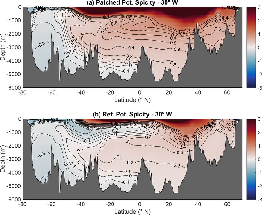
R. Tailleux: Spiciness theory revisited                                                                                              205

such points, temperature becomes approximately passive and
therefore the most natural definition of spiciness as pointed
out by Stipa (2002). At such points, however, the Jackett and
McDougall (1985) variable, like the Flament (2002) variable,
behaves like salinity, causing the Jacobian of the transforma-
tion ∂(τjmd , γ )/∂(S, θ ) to vanish, which seems unphysical.
                                                             0 ,
The ability of different kinds of anomalies, namely τν0 , τjmd
       0
and S , to characterise water mass contrasts and intrusions is
discussed in the second part of the Jackett and McDougall
(1985) paper. Interestingly, they find that even though the
spiciness as state functions τ ν , τjmd , and S behave quite dif-
ferently from each other in (S, θ ) space, their anomalies ex-
hibit in contrast only small differences, at least when esti-
mated for individual soundings. In this paper, I show that this
property actually appears to be satisfied much more broadly,
as illustrated in Fig. 12 and further discussed in the text.
   Orthogonality in (S, θ ) space – despite its usefulness or
necessity remaining a source of confusion and controversy           Figure 1. Comparison of different spiciness as state functions along
– has nevertheless been central to the development of spici-        30◦ W in the Atlantic Ocean: (a) a new form of potential spici-
ness theory. Recently, Huang et al. (2018) attempted to re-         ness τref = τ‡ (SA , 2, pr ) referenced to a variable reference pres-
habilitate the Veronis (1972) form of orthogonality by ar-          sure pr (S, θ). This spiciness variable is similar to the McDougall
guing that without imposing it, it is otherwise hard to de-         and Krzysik (2015) spiciness variable and defined in Sect. 3. The
fine a distance in (S, θ ) space. This argument is uncon-           variable reference pressure pr is defined in Sect. 2 and illustrated
vincing, however, because the concept of distance in math-          in panel (a) of Fig. 3. (b) The Huang et al. (2018) potential spicity
ematics does not require orthogonality; it only requires the        referenced to the same variable reference pressure pr as in (a), de-
introduction of a positive definite metric d(x, y), i.e. one        noted by πref in the paper; (c) Absolute Salinity; (d) Conservative
                                                                    Temperature. White contours in (c) and (d) (shown as brown con-
satisfying the following: (1) d(x, y) ≥ 0 for all x and y;
                                                                    tours in a and b) represent selected isocontours of a density-like
(2) d(x, y) = 0 is equivalent to x = y; (3) d(x, y) = d(y, x);                 T
                                                                    variable γanalytic similar to the Tailleux (2016b) thermodynamic
and (4) d(x, y) ≤ d(x, z) + d(z, y), the so-called triangle in-
equality. As a result, there is an infinite number of ways          neutral density variable γ T . The construction and implementation
                                                                         T
                                                                    of γanalytic are described in Sect. 2. These isocontours – the same in
to
q define distance in (S, θ ) space. For instance, d(A, B) =         all panels – are only labelled in (d) for clarity.
  β02 (SA − SB )2 + α02 (θA − θB )2 , where α0 and β0 are some
constant reference values of α and β, is an acceptable def-
inition of distance. Likewise, any two non-trivial and inde-
                                                                    to have any particular advantage over salinity at picking
pendent material functions γq   (S, θ ) and ξ(S, θ ) could also
                                                                    up ocean water mass signals, although both variables are
be used to define d(A, B) = (γA − γB )2 + K02 (ξA − ξB )2 ,         superior to temperature in this respect. This is shown in
where K0 is a constant to express γ and ξ in the same sys-          Fig. 1, which compares the aptitude of (a) reference poten-
tem of units if needed, while γA is shorthand for γ (SA , θA ),     tial spiciness τref , (b) reference potential spicity πref , (c) Ab-
with similar definitions for γB , ξA , and ξB . In regards to       solute Salinity, and (d) Conservative Temperature for visu-
the 45◦ orthogonality proposed by Jackett and McDougall             alising the water masses of the Atlantic Ocean along the
(1997) and Flament (2002), while it is true that it is un-          30◦ W section, the four main ones of which are North At-
affected by a re-scaling of the S and θ axes plaguing the           lantic Deep Water (NADW), Antarctic Intermediate Water
Veronis (1972) form of orthogonality, it is destroyed by the        (AAIW), Antarctic Bottom Water (AABW), and Mediter-
subtraction of any function of potential density while also         ranean Intermediate Water (MIW). The WOCE climato-
causing the above-mentioned loss of invertibility where α           logical dataset (Gouretski and Koltermann, 2004; avail-
vanishes. In any case, it is unclear why Jackett and Mc-            able at: http://icdc.cen.uni-hamburg.de/1/daten/index.php?
Dougall (1997) sought to impose the 45◦ orthogonality to            id=woce&L=1, last access: 25 January 2021) has been used
τjmd , since it is a priori
                        R not necessary
                                 R       to satisfy the above-      for this figure and for all calculations throughout this pa-
mentioned constraint dτjmd = β dS on isopycnal surfaces             per. The link between τref and πref as well as the spiciness
(in the sense that if one particular τjmd solves the problem,       and spicity variables of McDougall and Krzysik (2015) and
any τjmd → τjmd − τr (γ ) will also solve it).                      Huang et al. (2018) is explained in the next two sections.
   From a purely empirical viewpoint, neither spiciness             Figure 1 shows that while all variables are able to pick up
(however defined) nor Huang et al. (2018) spicity appears           the AABW signal similarly well, they differ in their ability
                                                                    to pick up the AAIW signal. Indeed, AAIW is most promi-

https://doi.org/10.5194/os-17-203-2021                                                               Ocean Sci., 17, 203–219, 2021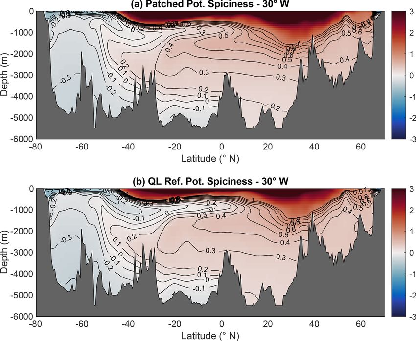
206                                                                                          R. Tailleux: Spiciness theory revisited

nently displayed in the salinity field, followed by πref and
τref , with Conservative Temperature a distant last, based on
how well defined the signal is and how far north it can be
tracked. In regards to NADW and MIW, they can be clearly
identified in all variables but temperature.
   Since salinity satisfies neither form of orthogonality, it is
natural to ask which properties make it superior to spiciness
and spicity as a water mass indicator. Because two signals
are visually most easily contrasted when their respective iso-
contours are orthogonal to each other, it is natural to ask
whether salinity could owe its superiority to being on aver-
age more orthogonal to density than other variables in phys-
ical space. To test this, the median angle between ∇γ and
∇ξ estimated for all available points of the WOCE dataset
was chosen as an orthogonality metric and computed for the
four spiciness as state functions (ξ ) considered. The result is
                                                                                                       T
                                                                      Figure 2. Median angle between ∇γanalytic and ∇ξ (blue bars) as
displayed in Fig. 2 (represented by the blue bars) for both
the global ocean (top panel) and the 30◦ W Atlantic section                                 T
                                                                      well as between ∇γanalytic  and ∇ξ 0 (red bars) for ξ = SA , ξ = τref ,
only (bottom panel). The median angle between ∇γ and ∇ξ               ξ = πref , and ξ = 2. Panel (a) takes into account all available data
was favoured over other metrics of orthogonality owing to             points of the WOCE dataset, whereas (b) only accounts for the data
its ability to rank the spiciness as state functions in the same      points making up the 30◦ W Atlantic Ocean section. See Sect. 4 for
order as the subjective visual determination of their ability as      details of the construction of ξ 0 . While the orthogonality to density
water mass indicators based on Fig. 1, with salinity first, πref      of spiciness as state functions depends sensitively on the variable
                                                                      considered (blue bars), this is much less the case of the correspond-
second, τref third, and temperature last. In this paper, this idea
                                                                      ing spiciness as anomalies, as seen by the similar magnitude exhib-
will be further explored by investigating whether the gener-
                                                                      ited by the red bars.
ally observed superior ability of ξ 0 over ξ as a water mass
indicator can be attributed to its increased orthogonality to
γ . (The results turn out to be inconclusive.)                        sure field pr (S, θ ), it can only be used in conjunction with
   The main aim of this paper is to explore the above ideas           spiciness as state functions whose dependence on pressure is
further and to clarify their inter-linkages. One of its key           sufficiently detailed. While this is the case of the Huang et al.
points is to emphasise that spiciness is a property, not a sub-       (2018) spicity variable, this is not the case of the McDougall
stance, and hence that it is spiciness as an anomaly rather           and Krzysik (2015) spiciness variable, which is only defined
than spiciness as a state function that is the relevant concept       for three discrete reference pressures, namely 0, 1000, and
to quantify water mass contrasts. This important point was            2000 dbar. To remedy this problem, Sect. 3 discusses the
recognised early on by Jackett and McDougall (1985) and               construction of a mathematically explicit spiciness variable
McDougall and Giles (1987) but for some reason has since              τ‡ (S, θ, p), which closely mimics the behaviour of the Mc-
been systematically overlooked in most of the recent spici-           Dougall and Krzysik (2015) variable in most of (S, θ ) space.
ness theory literature devoted to the construction of dedicated       As a result, two new potential spiciness and spicity variables
spiciness-as-a-state-function variables; e.g. Flament (2002),         referenced to the non-constant reference pressure pr (S, θ ),
McDougall and Krzysik (2015), Huang (2011), and Huang                 denoted by τref and πref , respectively, are introduced in this
et al. (2018). This is problematic because it has resulted in         paper. These are the variables depicted in Fig. 1a and b. Sec-
a disconnect between spiciness theory and its applications.           tion 4 discusses the links between the zero of spiciness, the
Section 2 emphasises the result that it is the degree of neu-         definition of a notional spiceless ocean, the construction of
trality of the density variable γ serving to define density-          spiciness anomalies, the orthogonality to density in physical
compensation that determines the degree of dynamical in-              space, and whether it is possible to meaningfully compare
ertness of spiciness variables ξ , not the properties of ξ itself.    the spiciness of two water samples that do not belong to the
Because the Tailleux (2016b) thermodynamic neutral density            same density surface. Finally, Sect. 5 summarises the results
γ T is currently the most neutral material density-like vari-         and discusses their implications and any further work needed.
                                                           T
able available, a new implementation of it, denoted γanalytic     ,
is proposed for use in spiciness studies. In contrast to γ ,    T
  T
γanalytic can be estimated with only a few lines of code and
is therefore much simpler to use in practice, while also be-
ing smoother and somewhat more neutral than γ T . Because
  T
γanalytic relies on the use of a non-constant reference pres-

Ocean Sci., 17, 203–219, 2021                                                                https://doi.org/10.5194/os-17-203-2021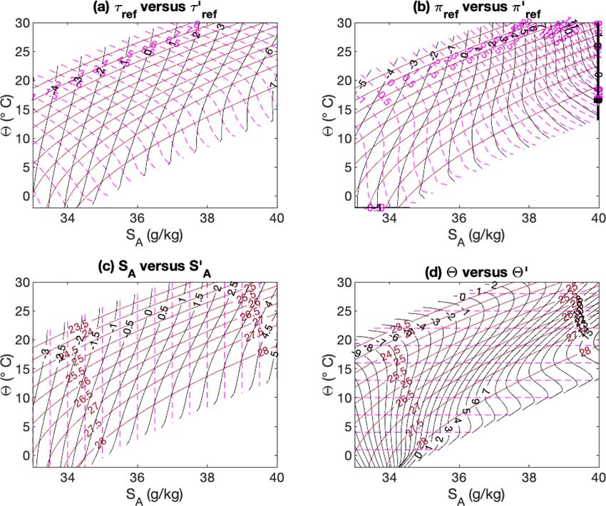
R. Tailleux: Spiciness theory revisited                                                                                          207

2     On the choice of isopycnal surfaces for spiciness              material density variable γ (S, θ ) maximising neutrality (al-
      studies                                                        though this will not come as a surprise to most oceanogra-
                                                                     phers).
2.1    Dynamical inertness of spiciness and neutrality
                                                                     2.2   A new implementation of thermodynamic neutral
As mentioned above, density-compensated thermohaline                       density for spiciness studies and water mass
variations are truly passive only if defined along surfaces of             analyses
constant in situ ρ. However, because such surfaces are sen-
sitive to pressure variations, it is useful in practice to seek a    Until recently, isopycnal analysis in oceanography has re-
purely material proxy γ = γ (S, θ ) of in situ density, which        lied on two main approaches: the use of vertically stacked
can also be used to capture the active part of S and θ . By          potential densities referenced to a discrete set of reference
introducing an as yet undetermined additional spiciness as a         pressures “patched” at the points of discontinuity following
state function, ξ , to capture the passive part of S and θ , in      Reid (1994), also called patched potential density (PPD), and
situ density may thus be rewritten as a function of the new          the use of empirical neutral density γ n proposed as a con-
(γ , ξ, p) coordinates as ρ = ρ(S, θ, p) = ρ̂(γ , ξ, p), with a      tinuous analogue of patched potential density by Jackett and
hat being used for the (γ , ξ, p) representation of any func-        McDougall (1997). Neither variable is exactly material, how-
tion of (S, θ, p). By using the so-called Jacobi method (see         ever. For PPD, this is because the points of discontinuities at
e.g. Appendix A of Feistel, 2018), Tailleux (2016a) showed           which potential density is referenced to different reference
that the partial derivatives of ρ̂ with respect to γ and ξ are       pressures are a source of non-materiality; see deSzoeke and
given by                                                             Springer (2009). For γ n , this is because such a variable also
                                                                     depends on horizontal position and pressure, although a way
∂ ρ̂   ∂(ρ̂, ξ )   1 ∂(ξ, ρ) Jγ                                      to remove the pressure dependence was recently proposed by
     =           =           =   ,                            (1)
∂γ     ∂(γ , ξ ) J ∂(S, θ )    J                                     Lang et al. (2020).
∂ ρ̂   ∂(γ , ρ̂)   1 ∂(ρ, γ ) Jξ                                        Recently, Tailleux (2016b) pointed out that Lorenz refer-
     =           =           = ,                              (2)
∂ξ     ∂(γ , ξ ) J ∂(S, θ )    J                                     ence density ρLZ (S, θ ) = ρ(S, θ, pr (S, θ )) that enters Lorenz
                                                                     (1955) theory of available potential energy (APE) (see
where Jγ = ∂(ξ, ρ)/∂(S, θ ), Jξ = ∂(ρ, γ )/∂(S, θ ), and J =         Tailleux, 2013b for a review) could be viewed as a gener-
∂(ξ, γ )/∂(S, θ ). To clarify the conditions controlling the pas-    alisation of the concept of potential density referenced to
sive character of ξ , it is useful to derive the following expres-   the pressure pr (S, θ ) that a parcel would have in a notional
sion for the neutral vector N in (γ , ξ, p) coordinates:             reference state of rest. A computationally efficient approach
         g                  g                                      to estimate the reference density and pressure vertical pro-
N =−        ∇ ρ̂ − ρ̂p ∇p = − ρ̂γ ∇γ + ρ̂ξ ∇ξ ,               (3)    files ρ0 (z) and p0 (z) that characterise the Lorenz reference
         ρ̂                  ρ̂
                                                                     state was proposed by Saenz et al. (2015). Once the latter
where ρ̂p = ∂ ρ̂/∂p, ρ̂γ = ∂ ρ̂/∂γ , and ρ̂ξ = ∂ ρ̂/∂ξ . Because     are known, the reference pressure pr = p0 (zr ) is simply ob-
the Jacobian J is invariant upon the transformation ξ → ξ −          tained by solving the Tailleux (2013a) level neutral buoyancy
ξr (γ ), the expression for N may alternatively be written in        (LNB) equation,
terms of ∇γ and ∇ξ 0 = ∇(ξ − ξr (γ )) as follows:
                                                                 ρ(S, θ, p0 (zr )) = ρ0 (zr ),                                (5)
          g              dξr              0
N =−           ρ̂γ + ρ̂ξ       ∇γ + ρ̂ξ ∇ξ .                 (4)     for the reference depth zr . As it turns out, ρLZ happens to be
          ρ              dγ
                                                                     quite neutral away from the polar regions where fluid parcels
Physically, the condition for ξ or ξ 0 to be dynamically inert       are close to their reference position. However, like in situ
is that it does not affect ρ̂, which mathematically requires         density, ρLZ is dominated by compressibility and its depen-
ρ̂ξ = 0. Equations (3) and (4) show this is equivalent to γ          dence on pressure. Tailleux (2016b) defined the thermody-
being exactly neutral. Equation (2) shows that this can only         namic neutral density variable,
be the case if ∂(ρ, γ )/∂(S, θ ) = 0. As is well known, this
condition can never be completely satisfied in practice be-          γ T = ρ(S, θ, pr ) − f (pr ),                                (6)
cause of thermobaricity, i.e. the pressure dependence of the
                                                                     as a modified form of Lorenz reference density empirically
thermal expansion coefficient (McDougall, 1987; Tailleux,
                                                                     corrected for pressure and realised that the empirical correc-
2016a). The above conditions thus establish that the degree
                                                                     tion function f (pr ) could be chosen so that γ T closely ap-
of dynamical inertness of ξ is controlled by the degree of
                                                                     proximates Jackett and McDougall (1997) empirical neutral
non-neutrality of γ . This is an important result for two rea-
                                                                     density γ n outside the ACC1 .
sons. First, it shows that the degree of dynamical inertness of
ξ is not determined by its properties (such as orthogonality)           1 The software used to compute γ n was obtained from the TEOS-
but by those of γ . Second, it provides new rigorous theoreti-       10 website at http://www.teos-10.org/preteos10_software/neutral_
cal arguments for justifying the pursuit of a globally defined       density.html (last access: 25 January 2021).

https://doi.org/10.5194/os-17-203-2021                                                               Ocean Sci., 17, 203–219, 2021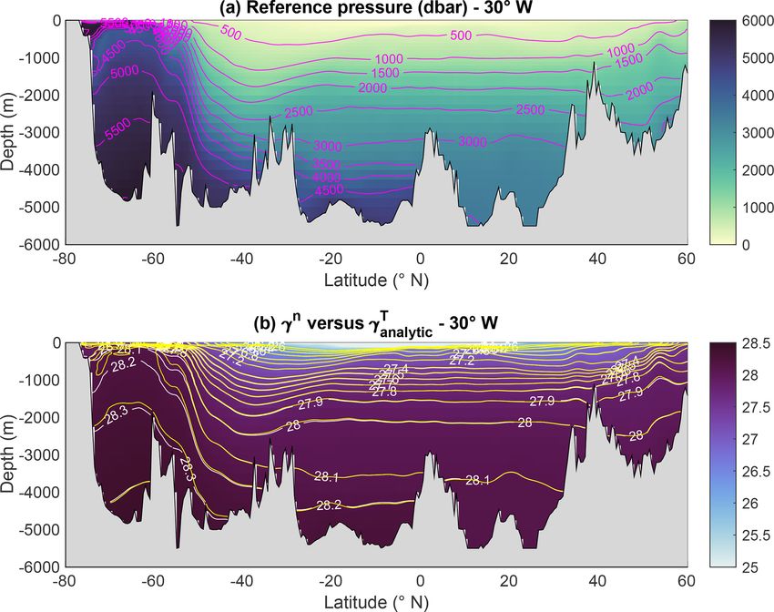
208 R. Tailleux: Spiciness theory revisited
Thermodynamic neutral density γ T is attractive because
it is as far as we know the most neutral purely material
density-like variable around. Unlike PPD, it varies smoothly
and continuously across all pressure ranges. Moreover, it
also provides a non-constant reference pressure pr (S, θ ) that
can serve to define potential spiciness and potential spicity
variables possessing the same degree of smoothness as γ T ,
whose construction is discussed in Sect. 3. At present, γ T is
therefore the most natural choice for use in spiciness stud-
ies since γ n , which, although somewhat more neutral, is not
purely material. However, the Tailleux (2013b) original im-
plementation of γ T is a multi-step process starting with the
computation of the Lorenz reference state, which, although
made relatively easy by the Saenz et al. (2015) method, is
computationally involved and therefore not necessarily eas-
ily reproducible by others. To circumvent these difficulties, I
am proposing here an alternative construction of γ T , called
T
γanalytic , which by contrast is easily computed with only a
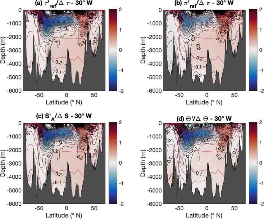
few lines of code while also being smoother and somewhat Figure 3. (a) Atlantic section along 30◦ W of the variable reference
more neutral than γ T . The proposed approach relies on using pressure pr = pr (SA , 2) = p0 (zr ) used for the construction of po-
analytic profiles for ρ0 (z) and p0 (z) instead of determining tential spiciness τ‡ (S, θ, pr ). (b) Atlantic section along 30◦ W of
these empirically, given by the Jackett and McDougall (1997) empirical neutral density vari-
able γ n . The white labelled contours represent selected isolines of
γ n , while the unlabelled yellow contours represent the same isolines
a(z + e)b+1 T
ρ0 (z) = + cz + d, (7) but for γanalytic .
b+1
a(z + e)b+2 cz2
p0 (z) = g +
(b + 1)(b + 2) 2
ae b+2
+dz − , (8)
(b + 1)(b + 2)
where z is positive depth increasing downward. The ref-
erence density profile ρ0 (z) depends on five parameters
(a, b, c, d, e), which were estimated by fitting the top-down
Lorenz reference density profile of Saenz et al. (2015). The
results of the fitting procedure are given in Table A1. As to
the empirical pressure correction f (p) entering Eq. (6), it is
chosen as a polynomial of degree 9 of the normalised pres-
sure (p − pm )/1p and given by the following expression:
9 9−n
X p − pm
f (p) = an . (9)
n=1
1p
The values of the coefficients an , pm , and 1p, as well as
estimates of confidence intervals returned by the fitting pro-
cedure are given in Appendix A. Figure 4. Atlantic sections along 30◦ W of the effective diffusivity
A full account of the performances and properties of of (a) the Jackett and McDougall (1997) empirical neutral density
T T
γanalytic will be reported in a forthcoming paper and is there- γ n , (b) analytic thermodynamic neutral density γanalytic , (c) poten-
fore outside the scope of this paper. Here, I only show two tial density σ1 , and (d) potential density σ2 . The white masked ar-
illustrations that are sufficient to justify the usefulness of eas flag regions where Kf > 10−5 m2 s−1 , which is widely used
T
γanalytic for the present purposes. Thus, the top panel of Fig. 3 as a threshold indicating large departure from non-neutrality. These
T
show that γanalytic is in general significantly more neutral than stan-
depicts the reference pressure field pr (S, θ ) = p0 (zr ) along
30◦ W in the Atlantic Ocean, while the bottom panel demon- dard potential density variables, while it is also similarly neutral as
strates the very close agreement between γ T and γ n outside γ n north of 50◦ S.
the Southern Ocean along the same section (the calculations
Ocean Sci., 17, 203–219, 2021 https://doi.org/10.5194/os-17-203-2021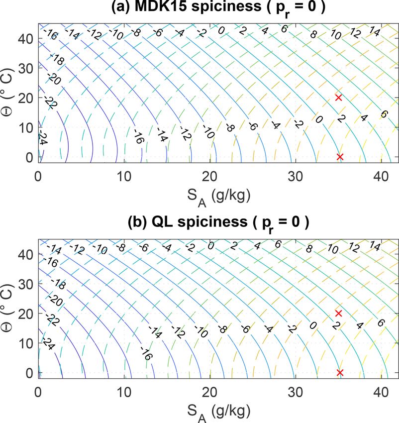
R. Tailleux: Spiciness theory revisited                                                                                                    209

presented actually make use of the new thermodynamic stan-
dard and use Absolute Salinity SA and Conservative Tem-
perature 2; see Pawlowicz et al., 2012; IOC et al., 2010).
Similarly good agreement was also verified in other parts
of the ocean (not shown). Figure 4 depicts latitude–depth
sections along 30◦ W in the Atlantic Ocean of the effec-
tive diffusivity Kf = Ki sin2 (N, ∇γ ) introduced by Hochet
et al. (2019), a metric for the degree of non-neutrality simi-
lar to the concept of fictitious diffusivity used by Lang et al.
                                      T
(2020) and others, for (a) γ n , (b) γanalytic , (c) σ1 , and (d) σ2 .
As before, N is the neutral vector, γ the density-like vari-
able of interest, and (N, ∇γ ) the angle between N and ∇γ .
The effective diffusivity Kf is conventionally defined using
Ki = 1000 m2 s−1 , a notional isoneutral turbulent mixing co-
efficient typical of observed values. It has become conven-
tional to use the value Kf = 10−5 m2 s−1 as the threshold
separating acceptable from annoyingly large degrees of non-
neutrality. By this measure, Fig. 4b shows that unlike σ1 and
                                    T                                    Figure 5. (a) Patched potential spicity referenced to the relevant ref-
σ2 , the degree of neutrality of γanalytic   is uniformly accept-
                                                                         erence pressure appropriate to the pressure range of fluid parcels;
able everywhere in the water column north of 50◦ S, where                (b) potential spicity referenced to the variable reference pressure
it is comparable to that of γ n . How to adapt the McDougall             pr (SA , 2). Referencing potential spicity to the variable reference
and Krzysik (2015) and Huang et al. (2018) potential spici-              pressure pr significantly increases its ability as a water mass indi-
                                                        T
ness and spicity variables to be consistent with γanalytic     is dis-   cator, especially with respect to the representation of AAIW.
cussed in the next section.

3     On the construction and estimation of potential
                                                                                                       J                 J
      spiciness-as-state-function variables                              di ξ = ξS di S + ξθ di θ =         γS di S = −       γθ di θ
                                                                                                      γS γθ             γS γθ
Since spiciness is a water mass property that can a priori                         J
be measured in terms of the isopycnal variations of any ar-                  =          (γS di S − γθ di θ ) ,                             (10)
                                                                                 2γS γθ
bitrary function ξ(S, θ ) independent of density, an impor-
tant question in spiciness theory is whether there is any real           where ξS = ∂ξ/∂S, ξθ = ∂ξ/∂θ, γθ = ∂γ /∂θ , and γS =
physical justification or benefits for introducing the kind of           ∂γ /∂S using the fact that by construction γS di S +γθ di θ = 0,
dedicated spiciness as state functions discussed by Veronis              with J = ∂(ξ, γ )/∂(S, θ ) being the Jacobian of the transfor-
(1972), Jackett and McDougall (1985), Flament (2002), Mc-                mation (S, θ ) → (ξ, γ ) as before. Equation (10) establishes
Dougall and Krzysik (2015), Huang (2011), and Huang et al.               the following.
(2018). Assuming that this is the case, how can existing                   1. di ξ is proportional to the elemental imperfect differ-
spiciness and spicity variables be adapted to be used consis-                 ential δτ = γS di S = −γθ di θ = 12 (γS di S − γθ di θ ) with
                T
tently with γanalytic and the non-constant reference pressure                 proportionality factor J /(γS γθ ) for all spiciness as state
pr (S, θ ) defined in the previous section, given that existing               functions, ξ . The two quantities γS di S and γθ di θ have
codes for computing such variables are in general limited to                  the same physical units; they can thus be regarded as
a few discrete reference pressures?                                           the basic building blocks for the construction of any
                                                                              spiciness-as-state-function variable if so desired.
3.1    Mathematical problems defining spiciness as state
       functions                                                           2. di ξ is unaffected by the transformation ξ → ξ − ξr (γ ),
                                                                              where ξr (γ ) is any arbitrary function of γ , so that both
To examine the benefits that might be attached to a particular                ξ and ξ − ξr (γ ) have identical isopycnal variations. The
choice of spiciness as a state function ξ(S, θ ) for studying                 benefit of imposing some particular property on ξ , such
water mass contrasts, it is useful to establish some general                  as orthogonality to γ , is therefore not obvious since
properties about what controls its isopycnal variations. By                   such a property cannot in general be satisfied by both
denoting di the restriction of the total differential operator to             ξ and ξ − ξr (γ ).
an isopycnal surface γ = constant, the isopycnal variations
of the latter may be written in the following equivalent forms:          According to Eq. (10), the main quantity determining the
                                                                         properties of the spiciness as a state function ξ is the Ja-
                                                                         cobian J . The generic mathematical problem determining ξ

https://doi.org/10.5194/os-17-203-2021                                                                     Ocean Sci., 17, 203–219, 2021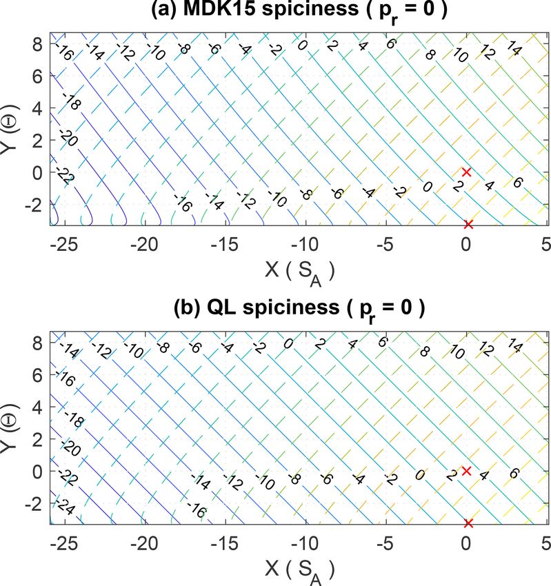
210                                                                                      R. Tailleux: Spiciness theory revisited

may therefore be written in the form                                expected, given the six transition points of discontinuities at
                                                                    p = 250, 750, 1500, 2500, 3500, and 4500 dbar). This shows
      ∂ξ      ∂ξ                                                    that the use of the variable reference pressure pr (SA , 2) has a
γθ       − γS    = J (S, θ ).                               (11)
      ∂S      ∂θ                                                    dramatic impact on the ability of spicity to pick up the water
                                                                    mass signals of the Atlantic Ocean. This is especially evi-
Eq. (11) can be recognised as a standard quasi-linear partial
                                                                    dent for the AAIW signal, which is only vaguely apparent in
differential equation amenable to the method of characteris-
                                                                    patched potential spicity, while being nearly as well defined
tics. Its general solution is defined up to some function ξr (γ )
                                                                    in πref as in the salinity field. This suggests that it is more
depending on the boundary conditions imposed ξ . In the im-                                                        T
                                                                    advantageous to use potential spicity with γanalytic   than with
portant particular cases in which ξ = θ and ξ = S, the Jaco-
                                                                    patched potential density.
bian and amplification factors are given by

          ∂γ       J       1                                        3.3   Construction of reference potential spiciness τref
ξ =S → J =     →        = ,                                 (12)
          ∂θ      γS γθ   γS                                        The Jackett and McDougall (1985) spiciness as a state func-
            ∂γ        J      1                                      tion τ is designed so that its isopycnal variations are con-
ξ =θ → J =−     →         =− .                              (13)
            ∂S      γS γθ    γθ                                     strained to satisfy the following mathematically equivalent
                                                                    relations:
Eqs. (12) and (13) exemplify the two main kinds of behaviour
of spiciness as state functions. For salinity-like ξ , the Jaco-    di τ = 2βdi S = 2αdi θ = βdi S + αdi θ,                     (14)
bian varies as γθ and is therefore quite non-uniform, with
loss of invertibility where γθ = 0; however, the scaling factor     where, as before, di is the restriction of the total differen-
J /(γS γθ ) varies as 1/γS and therefore varies little in (S, θ )   tial operator to the isopycnal surface γ (S, θ ) = constant and
space. This is the opposite for temperature-like ξ , for which      where α and β are the haline contraction and thermohaline
it is the Jacobian that is approximately constant and the scal-     expansion coefficients. In Jackett and McDougall (1985),
ing factor J /(γS γθ ) = −1/γθ that varies non-uniformly. To a      density surfaces are approximated in terms of σ0 , but the
large extent, these opposing behaviours characterise the Mc-        use of patched potential density is implicit in the more re-
Dougall and Krzysik (2015) and Huang et al. (2018) spici-           cent paper by McDougall and Krzysik (2015). By comparing
ness and spicity variables. Which behaviour is preferable           Eq. (14) with Eq. (10), it can be seen that the Jackett and Mc-
cannot be determined without bringing in additional physi-          Dougall (1985) construction implies a constant proportional-
cal considerations discussed in Sect. 4 and the Conclusions.        ity factor J /(ρS ρθ ) = 2. This in turn implies for the Jacobian
                                                                    and quasi-linear PDE satisfied by τ
3.2     Construction of reference potential spicity πref
                                                                          2ρS ρθ           τS τθ
The Huang et al. (2018) spicity variable π(SA , 2) is designed      J=           = −2ραβ →   −   = 2.                           (15)
                                                                            ρ              β   α
to enforce the Veronis (1972) definition of orthogonality in
the re-scaled SA and 2 coordinates X(SA ) = ρ0 β0 SA and            To solve the quasi-linear PDE Eq. (15), Flament (2002) and
Y (2) = ρ0 α0 2, with α0 and β0 being representative constant       Jackett and McDougall (1985) further imposed τ to satisfy
values of the thermal expansion and haline contraction coef-        the so-called 45◦ orthogonality, which in practice amounts
ficients, respectively. The imposition of this form of orthog-      to assuming that the total differential of τ satisfies dτ ≈
onality ensures that the transformation (SA , 2) → (γ , π ) is      λ(βdS +αdθ ), with λ being some integrating factor. Flament
invertible everywhere in (SA , 2) space, which is not the           (2002) and Jackett and McDougall (1985) approached the
case of the 45◦ form of orthogonality considered by Jack-           problem somewhat differently, but their variables are nev-
ett and McDougall (1985), Flament (2002), and McDougall             ertheless approximately linearly re-scaled functions of each
and Krzysik (2015). Huang et al. (2018) provide a MAT-              other.
LAB subroutine, gsw_pspi(SA,CT,pr), to compute π                       Both Jackett and McDougall (1985) and Flament (2002)
as a function of Absolute Salinity and Conservative Temper-         provide polynomial expressions in powers of S and θ
ature at the discrete set of reference pressures pr = 0, 500,       for their potential spiciness variable, which are, however,
1000, 2000, 3000, 4000, and 5000 dbar. This provides suffi-         limited to a single reference pressure pr = 0. More re-
cient vertical resolution for computing the reference potential     cently, McDougall and Krzysik (2015) have provided the
spicity πref (SA , 2) = π(SA , 2, pr (SA , 2)) referenced to the    MATLAB subroutines (available at http://www.teos-10.org,
variable reference pressure pr (SA , 2) defined in the previous     last access: 25 January 2021) gsw_spice0(SA,CT),
section using shape-preserving spline interpolation, as illus-      gsw_spice1(SA,CT), and gsw_spice2(SA,CT) to
trated in Fig. 5b. By comparison, panel (a) shows the patched       compute potential spiciness at the three reference pressures
potential spicity obtained by stacking up potential spicity es-     pr = 0 dbar, pr = 1000 dbar, and pr = 2000 dbar, where SA
timated at the reference pressure appropriate to its pressure       is absolute salinity and CT conservative temperature. Be-
range (which appears to be smoother than might have been            cause this limited number of reference pressures is far from

Ocean Sci., 17, 203–219, 2021                                                            https://doi.org/10.5194/os-17-203-2021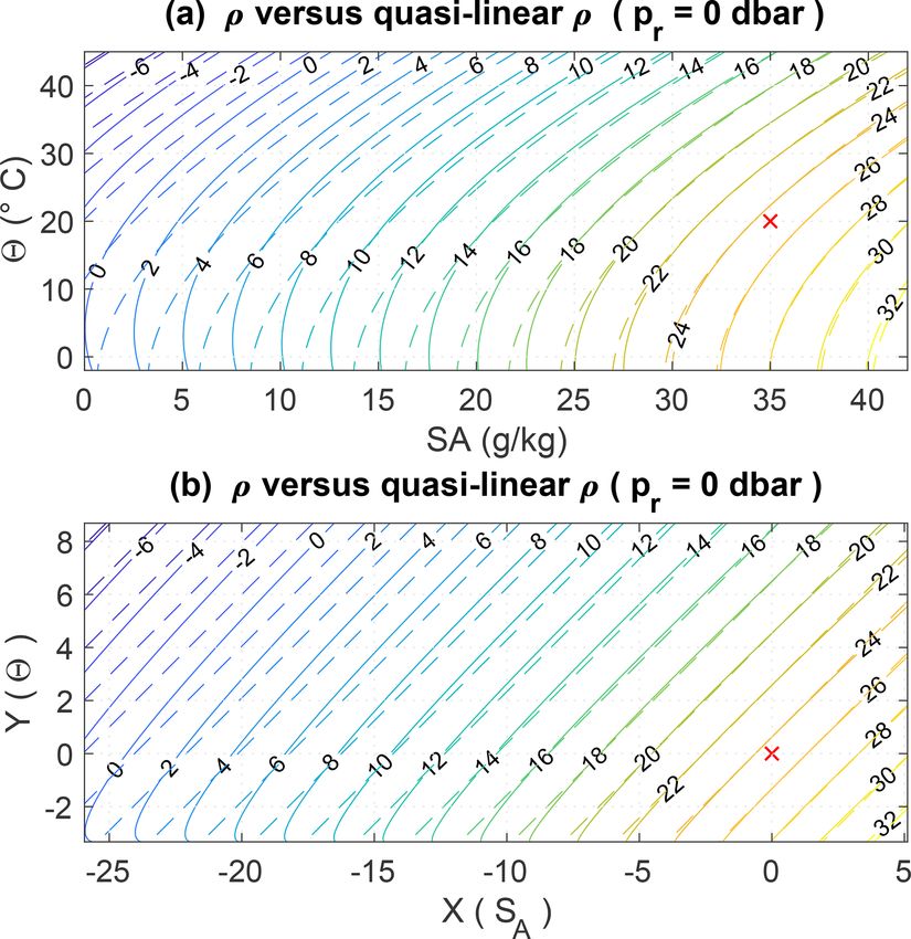
R. Tailleux: Spiciness theory revisited                                                                                           211

                                                                      are
                                                                      dτ‡ = ρ00 (β0 dS + α0 dθ ),

                                                                                    β0 α0
                                                                      di τ‡ = ρ00     +      βdi S,                               (19)
                                                                                    β    α
                                                                      where β0 = β(S, θ0 , pr ) and α0 = α(S0 , θ, pr ). For (S, θ )
                                                                      close enough to the reference point (S0 , θ0 ), di τ‡ ≈
                                                                      2ρ00 βdi S, which is equivalent to the differential problem that
                                                                      Jackett and McDougall (1985) set out to solve. An important
                                                                      difference with standard spiciness variables, however, is that
Figure 6. The re-scaled salinity and temperature X(SA ) and Y (2)
                                                                      the Jacobian associated with τ‡ is given by
expressing both quantities in a common system of density-like
units. Red dashed lines are the linear regressions of the equations   J = −ρ00 ρ (αβ0 + α0 β) < 0,                                (20)
X(SA ) = 0.74 SA − 26 and Y (2) = 0.26 2 − 4.5.
                                                                      and it differs from zero everywhere in (S, θ ) space. As to the
                                                                      pressure dependence of τ‡ , it is given by
ideal for computing potential spiciness τ (SA , 2, pr (SA , 2))
referenced to the variable reference pressure pr (SA , 2) un-         ∂τ‡
            T                                                             =ρ00 (κ(S, θ0 , p) − κ(S0 , θ, p)
derlying γanalytic , I have constructed an analytical proxy for       ∂p
the McDougall and Krzysik (2015) variable valid for the full
                                                                            − κ(Sref , θ0 , p) + κ(S0 , θref , p)) ,              (21)
range of pressures encountered in the ocean. The expression
for this proxy, called quasi-linear spiciness, is                     where κ(S, θ, p) = ρ −1 ∂ρ/∂p(S, θ, p). Equation (21) shows
                                                                      that ∂p τ‡ vanishes at the two reference points (S0 , θ0 ) and
τ‡ (S, θ, p) =X(S, p) + Y (θ, p) + τ0 (p)
                                                                    (Sref , θref ); it follows that, by design, τ‡ is only weakly de-
                       ρ(S, θ0 , p)                                   pendent on pressure and hence naturally quasi-material (that
             =ρ00 ln                  + τ0 (p).               (16)
                       ρ(S0 , θ, p)                                   is, approximately conserved following fluid parcels in the ab-
                                                                      sence of diffusive sources and sinks of S and θ ).
τ‡ is a linear combination of the non-linear re-scaled salin-            The McDougall and Krzysik (2015) spiciness and τ‡ are
ity and temperature coordinates X(S, p) and Y (θ, p) and of           compared in Figs. 7 and 8 in (SA , 2) space as well as in
reference function τ0 (p), whose expressions are                      the re-scaled (X, Y ) coordinates, respectively, at the refer-
                                                                    ence pressure pr = 0. The two variables can be seen to be-
                         ρ(S, θ0 , p)
X =X(S, p) = ρ00 ln                       ,                           have in essentially the same way, with the result also holding
                         ρ(S0 , θ0 , p)                               at pr = 1000 dbar and pr = 2000 dbar, except for cold tem-

                           ρ(S0 , θ, p)                               perature and low salinity values at which the Jacobian as-
Y =Y (θ, p) = −ρ00 ln                       ,           (17)
                           ρ(S0 , θ0 , p)                             sociated with McDougall and Krzysik (2015) spiciness van-

                   ρ(Sref , θ0 , p)
                                                                     ishes, while that associated with τ‡ does not. That both vari-
τ0 (p) = −ρ00 ln                      .                 (18)          ables approximately satisfy the 45◦ orthogonality is made
                   ρ(S0 , θref , p)
                                                                      obvious in the re-scaled (X, Y ) coordinates in Fig. 8; in-
These functions depend on some arbitrary reference con-               terestingly, this plot suggests that in situ density is approx-
stants, specified as follows: ρ00 = 1000 kg m−3 is chosen to          imately a linear function of X and Y , which is further ex-
give τ‡ the same unit as density, while τ0 (p) = τ (S0 , θ0 , p)      amined in Appendix B. Moving to physical space, Fig. 9
specifies the reference value of τ‡ at the reference point            compares the patched potential spiciness computed using the
(S0 , θ0 ). In principle, S0 and θ0 could also be made to depend      McDougall and Krzysik (2015) software (top panel) versus
on pressure p, but this complication is avoided for simplic-          the reference potential spiciness τref = τ‡ (SA , 2, pr (SA , 2))
ity. Figure 6 illustrates a particular construction of X(SA , p)      calculated with τ‡ . For patched potential spiciness, the tran-
and Y (2, p) based on the values S0 = 35 g kg−1 , 20 =                sition points of discontinuity were chosen at pr = 1000 and
20 ◦ C, and p = 0 dbar. The reference point (Sref , θref ) de-        2000 dbar. As for potential spicity, it also appears to be ad-
fines where τ‡ vanishes. The values Sref = 35.16504 g kg−1            vantageous to use potential spiciness with a variable pr , as it
and 2ref = 0 ◦ C were used to fix the zero of τ‡ as in Mc-            makes AAIW more marked and NADW somewhat more ho-
Dougall and Krzysik (2015). Figure 6 shows that while                 mogeneous. The effect of a variable pr on potential spiciness
Y (SA ) varies approximately linearly with SA , Y (2) clearly         is not as dramatic as for potential spicity, however, which
varies non-linearly with 2. Linear regression lines are also          is likely due to the weak pressure dependence of τ‡ noted
indicated to illustrate the departure from non-linearity.             above. In any case, the above analysis suggests that τ‡ is a
The total and isopycnal differentials of potential spiciness          useful proxy for the McDougall and Krzysik (2015) spici-
τ‡ (S, θ, pr ) referenced to the constant reference pressure pr       ness variable.

https://doi.org/10.5194/os-17-203-2021                                                                   Ocean Sci., 17, 203–219, 2021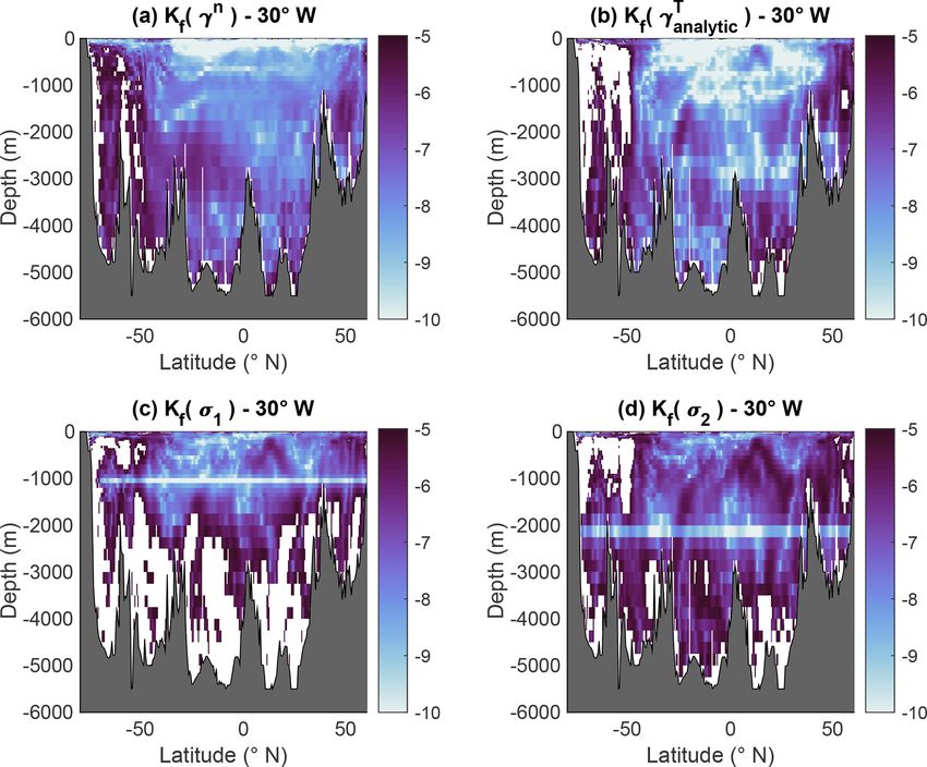
212                                                                                           R. Tailleux: Spiciness theory revisited

Figure 7. (a) Isocontours of the McDougall and Krzysik (2015)
spiciness variable referenced to the surface pressure (solid lines)    Figure 9. (a) Patched potential spiciness referenced to the three dis-
along with σ0 isocontours (dashed lines). (b) Isocontours of the       crete reference pressures provided by the McDougall and Krzysik
mathematically explicit quasi-linear spiciness variable introduced     (2015) software appropriate to their pressure ranges. (b) Quasi-
in this paper referenced to the surface pressure (solid lines) along   linear potential spiciness referenced to the variable reference pres-
with σ0 isocontours (dashed lines). The crosses indicate the refer-    sure pr = pr (SA , 2) = p0 (zr ). In contrast to spicity, the use of
ence point (SA , 2) = (35, 20) at which X = Y = 0 and the refer-       a variable reference pressure has little impact on the visual as-
ence point (SA , 2) = (35.16504, 0) at which both spiciness vari-      pect of spiciness, thus confirming the weak pressure dependence
ables are imposed to vanish.                                           of τ‡ (SA , 2, p).

                                                                       particular water masses to be analysed. Whether this point
                                                                       is well known is unclear because the distinction between
                                                                       a property and a substance is rarely evoked if ever in the
                                                                       spiciness literature. As a result, it follows that the usefulness
                                                                       of spiciness-as-a-state-function variables such as those of
                                                                       Jackett and McDougall (1985), Flament (2002), and Huang
                                                                       et al. (2018), which do not incorporate any information about
                                                                       the particular water masses to be analysed, is only limited
                                                                       to quantifying the relative differences in spiciness for fluid
                                                                       parcels that belong to the same density surface, as pointed out
                                                                       Timmermans and Jayne (2016). In other words, any differ-
                                                                       ence in spiciness for fluid parcels belonging to different den-
                                                                       sity surfaces predicted by such variables is physically mean-
                                                                       ingless. Physically, this limitation is associated with another
                                                                       key one, namely the impossibility to link a spiceless ocean
                                                                       to the zero value of a spiciness-as-a-state-function variable.
Figure 8. Same as Fig. 7 but with SA and 2 replaced by the re-         This is not surprising because the zero and other isovalues
scaled salinity and temperature coordinates X(SA ) and Y (2), in       of any spiciness as a state function are necessarily artificial
which the spiciness and density variables visually appear approxi-     since they are not informed by a physical consideration of
mately orthogonal to each other.                                       how to endow the relative spiciness of two fluid parcels that
                                                                       belong to different density surfaces with physical meaning.
                                                                       Here, a spiceless ocean is defined as a notional ocean in
4     Links between spiciness as a property, the zero of               which iso-surfaces of potential temperature, salinity, and po-
      spiciness, and orthogonality in physical space                   tential density would all coincide. It follows that in a spice-
                                                                       less ocean, any spiciness as a state function would have to be
As stated previously, it is important to recognise that spici-         a function of density only, for example ξ = ξr (γ ), which in
ness is not a substance but a property that cannot be described        general must differ from zero. This suggests that spiciness as
without taking into account empirical information about the            a property should be defined as the anomaly ξ 0 = ξ − ξr (γ ),

Ocean Sci., 17, 203–219, 2021                                                                https://doi.org/10.5194/os-17-203-2021
R. Tailleux: Spiciness theory revisited 213
as originally proposed by Jackett and McDougall (1985) and
McDougall and Giles (1987). Clearly, such an approach ad-
dresses the zero-of-spiciness issue, since it ensures that ξ 0
would vanish in a spiceless ocean, as desired. Moreover, it
also define spiciness as a property rather than as a substance
because although ξ 0 = ξ 0 (S, θ ) is a function of S and θ , it is
not truly a function of state owing to its dependence on the
empirically determined function of density ξr (γ ).
Because any function ξ(S, θ ) independent of γ is a po-
tential candidate for constructing a spiciness-as-a-property
ξ 0 = ξ − ξr (γ ) variable, the following questions arise.
1. Are there any benefits in constructing a dedicated spici-
ness as a state function ξ for the purpose of constructing
the anomaly ξ 0 = ξ −ξr (γ )? Are there any good reasons
to think that S 0 = S − Sr (γ ) and θ 0 = θ − θr (γ ) are not
suitable or insufficient for all practical purposes?
Figure 10. Non-linear regression between γanalytic T and various
2. Since neither the Veronis (1972) form of orthogonality
spiciness as state functions estimated for data restricted to the
nor the Jackett and McDougall (1985) 45◦ orthogonality
30◦ W Atlantic section (in red and orange): (a) potential reference
can be satisfied by ξ 0 , what is the physical justification spiciness τref , (b) potential reference spiciness πeref , (c) Conserva-
for imposing it on ξ in the first place? tive Temperature, and (d) Absolute Salinity. The non-linear regres-
sion curve is indicated in solid black and is described by a second-
3. In physics, the scale to measure some quantities is com- T
order polynomial in γanalytic . The yellow data points represent the
monly accepted to be arbitrary, which is why several
whole dataset for the global ocean for comparison.
scales (e.g. Kelvin, Celsius, and Fahrenheit) have been
developed over time to measure temperature, for in-
stance. To what extent is the problem of quantifying by means of a non-linear regression of ξ against γanalytic T .
spiciness as a property similar to or different from that A polynomial descriptor was preferred over using a simple
of constructing a temperature scale? isopycnal average as in Jackett and McDougall (1985) or
4. To what extent is the problem of deciding in favour of McDougall and Giles (1987) to ensure the smoothness and
T
differentiability of ξr (γanalytic ). To minimise the impact of
a particular choice of ξ one that can be constrained by
physical arguments as opposed to one that is fundamen- outliers, the robust bisquare least-squares provided by MAT-
LAB was used2 . Because a scatter plot of ξ against γanalyticT
tally arbitrary and therefore a matter of personal prefer-
ence? does not reveal any particular relation between the two vari-
ables if all the ocean data points are used, as shown in Fig. 10
5. Are there any additional constraints that ξ 0 = ξ − ξr (γ ) by the yellow points, the non-linear regression for obtaining
should satisfy beyond the zero-of-spiciness issue in or- T
the second-order polynomial ξr (γanalytic ) was restricted to the
der for relative difference in ξ 0 for fluid parcels that be- ◦
points making up the 30 W Atlantic section (indicated in red
long to different density surfaces to be considered phys- and orange), for which a relation is more apparent. The re-
ically meaningful? sulting function, depicted as the black solid line in Fig. 10,
was then used to construct ξ 0 in both thermohaline space in
Jackett and McDougall (1985) shed some light on some Fig. 11 and physical space in Fig. 12. Similarly as in Jack-
of the above issues by suggesting that the choice of ξ may ett and McDougall (1985), Fig. 11 shows that the signifi-
be less important than one would think. Indeed, they showed cant inter-differences in behaviour exhibited by the differ-
that the inter-differences in appropriately re-scaled anomaly ent ξ are considerably reduced for ξ 0 . The result is signifi-
0 , τ 0 , and S 0 were considerably reduced over
functions τjmd ν cantly more general than in Jackett and McDougall (1985),
those exhibited by τjmd , τν , and S, a potentially important however, since it pertains to a large part of (SA , 2) space as
result that does not appear to have received much atten- opposed to being limited to a few vertical soundings. In all
tion so far. The Jackett and McDougall (1985) conclusion plots in Fig. 11, ξ 0 (SA , 2) is shown to be an increasing func-
is only based on the comparison of two vertical soundings, tion of SA but decreasing function of 2, similarly as density
however, so it is necessary to examine it more systemati-
cally in order to assess its robustness. To that end, I con- 2 The MATLAB documentation page reviewing the various
structed particular examples of anomaly functions ξ 0 for the least-squares methods can be consulted at https://uk.mathworks.
four variables considered in the Introduction based on the use com/help/curvefit/least-squares-fitting.html (last access: 26 Jan-
of a second-order polynomial descriptor for ξr (γ ) obtained uary 2021).
https://doi.org/10.5194/os-17-203-2021 Ocean Sci., 17, 203–219, 2021You can also read