How Do Eutrophication and Temperature Interact to Shape the Community Structures of Phytoplankton and Fish in Lakes? - MDPI
←
→
Page content transcription
If your browser does not render page correctly, please read the page content below
water
Article
How Do Eutrophication and Temperature Interact to
Shape the Community Structures of Phytoplankton
and Fish in Lakes?
Liess Bouraï 1,2, *, Maxime Logez 1,2 , Christophe Laplace-Treyture 2,3        and
Christine Argillier 1,2
 1   Equipe Fonctionnement et Restauration des Hydrosystèmes Continentaux (FRESHCO), Risques,
     Ecosystèmes, Vulnérabilité, Environnement, Résilience (UR RECOVER), Institut National de la Recherche
     Pour L’agriculture, L’alimentation et L’environnement (INRAE), Aix Marseille University,
     F-13100 Aix-en-Provence, France; maxime.logez@inrae.fr (M.L.); christine.argillier@inrae.fr (C.A.)
 2   Pôle R&D Ecosystèmes Lacustres (ECLA), F-13100 Aix-en-Provence, France;
     christophe.laplace-treyture@inrae.fr
 3   UR EABX (Ecosystèmes Aquatiques et Changements Globaux), INRAE (Institut National de la Recherche
     Pour L’agriculture, L’alimentation et L’environnement), F-33612 Cestas, France
 *   Correspondence: liess.bourai@inrae.fr

 Received: 30 January 2020; Accepted: 9 March 2020; Published: 11 March 2020

 Abstract: Freshwater ecosystems are among the systems most threatened and impacted by
 anthropogenic activities, but there is still a lack of knowledge on how this multi-pressure environment
 impacts aquatic communities in situ. In Europe, nutrient enrichment and temperature increase due
 to global change were identified as the two main pressures on lakes. Therefore, we investigated
 how the interaction of these two pressures impacts the community structure of the two extreme
 components of lake food webs: phytoplankton and fish. We modelled the relationship between
 community components (abundance, composition, size) and environmental conditions, including
 these two pressures. Different patterns of response were highlighted. Four metrics responded
 to only one pressure and one metric to the additive effect of the two pressures. Two fish metrics
 (average body-size and biomass ratio between perch and roach) were impacted by the interaction
 of temperature and eutrophication, revealing that the effect of one pressure was dependent on the
 magnitude of the second pressure. From a management point of view, it appears necessary to
 consider the type and strength of the interactions between pressures when assessing the sensitivity of
 communities, otherwise their vulnerability (especially to global change) could be poorly estimated.

 Keywords: global change; nutrients; anthropogenic pressure stressor; interaction; multiple stressors;
 lake systems

1. Introduction
     Freshwater ecosystems are among the systems most threatened and impacted by anthropogenic
activities [1]. They are characterized by their high biodiversity [2], the erosion of which is considered
to be steeper than that of terrestrial ecosystems [3], which makes them more vulnerable. Aquatic
ecosystems are exposed to numerous anthropogenic stressors, be they physical (i.e., habitat degradation),
chemical, or biological (i.e. invasive species), which interact with global change and lead to additional
perturbations [4–8]. These multiple stressors compromise freshwater biodiversity and its associated
biological functions, and ultimately the services provided by these systems to our society [9,10].
     In Europe, monitoring associated with the implementation of the Water Framework Directive
(WFD; an environmental policy that aims to protect and restore continental aquatic systems) showed

Water 2020, 12, 779; doi:10.3390/w12030779                                       www.mdpi.com/journal/water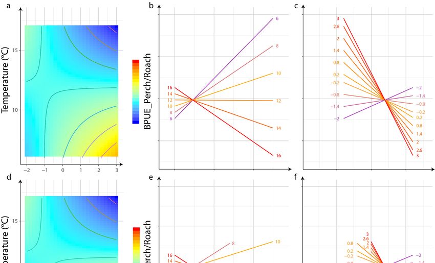
Water 2020, 12, 779                                                                                    2 of 17

that numerous aquatic ecosystems are impaired by human activities, with their ecological status
ranging from bad to moderate [4,11]. While the WFD calls for lakes (like all bodies of water) to be
in ’good ecological status’, the latest evaluation (2nd River Basin Assessment) showed that 45% of
lakes did not reach this status [12]. Unfortunately, in certain hydrographic basins, this percentage
may even reach 100%. The report of the European Environmental Agency [12] emphasized that lakes
are particularly impacted by nutrient enrichments, and also by climate change, more specifically by
temperature increases [4,12,13]. The impact of these two stressors is also the most studied. In their
review based on 219 studies, Nõges et al. [10] revealed that 78% dealt with nutrient impacts and 31%
with temperature effects, either solely or jointly.
     Nevertheless, although lakes rarely face a single pressure, few studies have looked at the
combined effects of several pressures, and even fewer have examined their interactions. Some results
concerned the cumulative effects of temperature and eutrophication on phytoplankton. Both pressures
affect phytoplankton abundance and composition [14–17]. For instance, Krosten et al. [18] showed
that temperature and nutrients both increase the relative abundance of cyanobacteria. However,
in some cases, related by Richardson et al. [19], this relation can be different, depending on the
lake type (morphological characteristics of the lake). Similarly, Jeppesen et al. [20] observed that
fish community composition changed as a result of these two pressures. Coldwater species were
replaced by warm-water-tolerant species owing to longer warm periods in summer and lower
oxygen concentrations.
     In most of these studies, when multi-stressors were considered, their combined effect was
commonly assumed to be additive, i.e., equal to the sum of the individual effects of the stressors
acting in isolation. This additive model is increasingly discussed in ecological systems in terms of
antagonistic and synergistic interactions [4,7,10,21,22]. Stressors can act in synergy when the combined
effect of stressors is greater than the sum of the impacts of individual stressors, whereas antagonistic
interactions occur when the combined effect of stressors is less than expected based on their individual
effects [23]. In situ, temperature and nutrient enrichment interaction is very often assumed to impact
biological communities, but it is rarely quantified or modelled (see Rigosi et al. [24] for exceptions).
This phenomenon is better studied in experimental conditions under which nutrient concentrations
and temperature can be controlled [21,25–27]. Nevertheless, from a management point of view, the
value of a study of this kind could be limited (e.g., the discrepancy between scales, other factors
involved, etc.), and without taking into account these interactions (if verified), the evaluation of the
lake status could be biased (e.g., [28]). In addition, knowledge of these interactive effects can be useful
in the implementation of management plans, with the ecological benefit resulting from efforts to reduce
interactive multi-stressors possibly giving rise to some ‘ecological surprises’ [5,29,30].
     The aim of this study was to assess whether: (i) temperature and eutrophication impact various
components (metrics) of the lake community, such as productivity and size structure, (ii) whether
these effects are additive, (iii) or whether they are multiplicative, i.e., whether the effect of one pressure
depends on the other pressure. We focused on two biological groups at the two ends of the trophic
chain that are representative of the lake community, are often used in bioindication, and are studied
in multi-stress conditions: phytoplankton and fish [7,10,31–34]. Moreover, a given pressure could
impact each biological element either directly or indirectly through cascade effects along the trophic
chain [17,35–37]. Hence, we could hypothesize similar responses to pressure from both trophic levels
expressed by the increase in primary productivity and, thus, fish productivity with temperature and
nutrients [37–40]. Similarly, we expected change to the community and a negative relationship between
temperature and sizes [35,41–43].
     This study was conducted at the macro-ecological scale, on a consistent dataset of 204 French
lakes to ensure large diversity in thermal and trophic conditions. The combined effect of temperature
and eutrophication was studied by comparing three statistical models: one considering only the effect
of lake morphology, a second model considering an additive effect of the two pressures, and a more
complex model considering the interaction between pressures.
Water 2020, 12, 779 3 of 17
2. Materials and Methods
2.1. Biological Data
The dataset comprised 204 French lakes, 48 natural lakes, and 156 reservoirs, for which biological
and environmental data were available and collected in a standardized manner.
Fish samples were collected according to the Norden gillnet standardized protocol [44] during the
period between July and mid-October. This protocol is based on a randomly stratified sampling design.
Benthic gillnets, 30 m in length, 1.5 m in height, composed of 12 panels with mesh sizes ranging from 5
to 55 mm knot-to-knot, were randomly distributed in the depth strata of the lakes. The gillnets were
set before sunset and lifted after sunrise to cover peaks of maximal fish activity [45,46]. All fish caught
were identified at the species level, then measured (total length in millimeters) and weighed (to the
nearest gram).
Phytoplankton was collected using a standardized method [47] and processed in laboratory
following the counting process of the European Standard NF15204 [48]. Four sampling campaigns a
year are recommended for each lake: three during the warmer period (between May and October) and
one in late winter. Phytoplankton was collected at the deepest point of the lakes, in the euphotic part
of the water column. Taxa were determined at the species level in the laboratory and their abundances
were weighted by taxa biovolume [49] using standard cell values defined in the software Phytobs [50],
or measured directly from the sample if the values were lacking. Additionally, chlorophyll-a was
collected from the euphotic zone during each sampling event and measured using the standard
methods NF-T 90-117 [49,51,52].
2.2. Biological Characterization
For each sampling occasion, ichthyofauna was characterized by eight metrics related to its density,
by its composition, and by the size of the individuals making up the communities. Density was
estimated by the number of individuals caught per sampling unit effort (expressed in square meters of
nets set during a 12-h night period; CPUE) and the total biomass caught per sampling unit effort (BPUE).
The ratio between the abundance of a predator, the perch (Perca fluviatilis), and the abundance of a prey,
the roach (Rutilus rutilus), was used as a proxy of the trophic equilibrium of the lakes [53,54]. These two
species are very common in French temperate lakes and generally abundant [55,56]. BPUEs and CPUEs
were calculated for both species and their ratios (BPUE_Perch/Roach and CPUE_Perch/Roach) were
computed for all the lakes where the two species occurred. In addition, the ratio of average perch to
roach body size (Average Perch/Roach Body Size) was calculated for each lake to measure the evolution
of ichthyofauna composition. The overall size of the fish community was assessed by the average size
of all the fish caught in the benthic gillnets in a lake. This metric is useful for comparing the average
difference in fish size between communities without differentiating between the processes behind it
(loss of the largest individuals, decrease in the size of all fish, increase of small species or individuals,
etc.) [57,58]. To investigate the processes involved in the change in size structure, the community size
spectra (CSS) were considered [59]. CSS represent a frequency distribution of individual body sizes
across size classes (defined on a log-scale) irrespective of taxonomy, through a linear regression relating
abundances to size classes on log scales. Two metrics were calculated: the midpoint and the slope
of the regression. The midpoint (CSS_Midpoint) value is an indicator of productivity of the system
and determines the level of richness of ecosystems. For instance, two communities can display the
same slope but different midpoints if the one has more fish than the other [60]. Slope (CSS_Slope) is
an indicator of the health of the community [60], for example, fish overexploitation will reduce the
abundance of large fish traduced by a high slope value.
Four metrics relating to density, composition, or size of phytoplankton communities were
considered. Phytoplankton total biomass was surrogated by the concentration of chlorophyll-a (Chl-a,
µg/L) in the euphotic zone. To limit the impact of seasonal variability, the Chl-a concentrations
of the three summer samples were averaged. The composition of phytoplankton was assessed byWater 2020, 12, 779 4 of 17
the abundances of cyanobacteria and golden alga (Chrysophytes). Cyanobacteria are assumed to
benefit from warmer temperatures and become dominant in higher nutrient concentrations, whereas
Chrysophyceae are assumed to prefer colder and less eutrophic conditions [41,61–63]. Their abundances
were weighted by taxa biovolume (considered as fixed) in order to calculated their respective biomass
(Cyano_Biovolume and Chryso_Biovolume), and expressed in cubic millimeters per liter (mm3 /L).
We then defined two size classes of phytoplankton, each taxon was classified as large or small,
irrespective of whether the taxon was considered larger or smaller than microphytoplankton, as
defined in the literature [64]. The ratio of the biomasses of large taxa on the biomasses of small taxa
in each lake was then calculated. This metric (phytoplankton size class) allows us to see, as with
ichthyofauna, whether the size structure of the phytoplankton community is affected by thermal and/or
eutrophic stress [41,42,62,65,66].
2.3. Environmental Data
The lakes were characterized by natural environmental variables potentially influencing
the structure of biological assemblages [67,68], i.e., physical/morphological characteristic of their
environment, and by stressors.
The dataset comprised 204 French lakes, 48 natural lakes and 156 reservoirs. This corresponds to
a diversity of lake throughout the French territory with morphological characteristics, ranging from
the plain lake to the mountain lake, from the shallow lake to the deep lake, and very varied in terms
of surface, area, the shape of the lake basin, and mean temperature or trophy level (details of the
calculation of the index below) (Table 1, see Supplementary Materials for more details).
Table 1. Characterization of the environmental variables of the lakes studied.
Environmental Variable Minimum–Maximum Mean (SD)
Altitude (m) 0–2061 404.8 (382.4)
Perimeter (m) 1.5 × 10³ –1.9 × 10⁵ 1.7 × 10⁴ (2.1 × 10⁴ )
Depth (m) 0.3–154.2 12.7 (16.6)
Area (km2 ) 0.1–577.1 6.1 (40.9)
Volume (m3 ) 1.3 × 10⁵ –8.9 × 10¹⁰ 5 × 10⁸ (6.2 × 10⁹ )
Ig (m/km) 0.1–155.7 8.1 (16.8)
Temperature (◦ C) 2.9–16.3 11.1 (2.2)
Eutrophication −2.0–3.1 −0.01 (1.1)
In order to limit the multi-collinearity between predictors (thus the redundancy between physical
variables), we ran a principal component analysis. Four variables emerged from this analysis and
characterized lake morphology: the mean depth (Depth, m), the area (Area, km2 ), the water volume
(Volume, m3 ), and the overall hill index (Ig, m/km). Ig was calculated from the maximum depth,
perimeter, and area [69,70] that characterizes the shape of the lake basin, according to the following
Equation (1):
Pmax
Ig = , (1)
Lr
with s
!2
0.282 1.128
Lr = Plake × × 1 + 1 − , (2)
1.128 KC
and
Plake
KC = 0.282 × √ , (3)
Alake
where Pmax is the maximum depth of the lake (m), Plake is its perimeter (km) and Alake its area (km2 ).
Two stressors were considered: temperature and eutrophication. Because water temperatures
were not available for all the lakes but are strongly correlated with air temperatures [71,72] (R2 = 0.82),Water 2020, 12, 779 5 of 17
we used the latter to characterize lake temperatures. To this end we used data from the SAFRAN
reanalysis [73,74], available at a spatial resolution of 8 km × 8 km. To integrate the difference of altitude
between grid cells and lakes, a correction of 6.5 × 10⁻³ C/m was applied.
Eutrophication was described by three variables: total phosphorous concentration (TP, µg/L),
nitrate concentration (NO3 , µg/L) and importance of non-natural land cover in the catchment area
(NNLC, percentage of the total catchment area). Phosphorus values range from 5 µg/L to 464 µg/L,
corresponding to trophic states classified from oligotrophic to hyper-eutrophic [75]. The nutrients
were sampled in the euphotic zone during the four same annual campaigns as for phytoplankton,
according to a standard sampling method. NNLC was defined as the percentage of non-natural areas
in the catchment and derived from the Corine Land Cover database [76]. This encompassed the
CLC categories: (1) artificial territories and (2) agricultural territories (without 23 grasslands) [77].
We summarized the information of these eutrophication measures in a synthetic index of eutrophication.
First, TP and NO3 were log-transformed, NNLC was transformed by the arcsin of the square root, and
then each variable was centered and reduced. The three transformed variables were averaged and
these values were centered and reduced to produce the synthetic index.
All the data used in this study were collected between 2005 and 2017 by research institutes or
water agencies, and centralized in a database by our laboratory.
To reduce the skewness of their distribution we log transformed maximum depth, lake area, lake
volume, Ig, BPUEs, CPUEs, Chl-a, and the biovolumes of cyanobacteria and Chrysophyceae.
2.4. Data Analysis
To assess the significance of the interactions of pressures on biological metrics we defined three
nested linear models related to three hypotheses [78]: (i) no pressure effect, (ii) additive effect of
pressures, and (iii) interaction of pressures (multiplicative effect of pressures). The first model related
the variability of biological metrics to physical variables only, metric ~ depth + area + Volume + Ig
corresponds to the environmental data block (called ‘environment’ in the next formulae); the second
model integrated the physical variables and the variable of pressures in an additive manner, metric ~
environment + temperature + eutrophication; the more complex model integrated the interaction
between temperature and eutrophication, metric ~ environment + temperature + eutrophication +
temperature interacting with eutrophication. The first model assumed that biological metric variability
depends only of the environmental conditions. The second model hypothesizes that the effect of
each pressure is independent of the other. In other words, whatever the level of the second pressure,
the magnitude of response to the first pressure will always be the same. Conversely, the interaction
included in the third model assumed that the effect magnitude of one pressure depends on the intensity
of the second pressure.
The effect of pressures and their behavior (additive or multiplicative) were tested on each fish
and phytoplankton metric by comparing models two by two with ANOVA (F-tests). First, we tested
model 3 vs. model 2, then, if the interaction was not significant, we tested model 2 vs. model 1
to verify the significance of the pressure effect on the metric variability (F-tests). Once the most
explanatory model was selected, we visually checked whether the linear model assumptions were
verified (i.e., homoscedasticity, normality of residuals). Only metrics for which more than 10% of the
variability of the biological metrics was explained were retained.
Finally, because it would have been difficult to forecast from coefficient values, if the interaction
was significant, we looked at its effect in graph form using graph effect display representation [79]. For
each graph, we represented how the expected metric values varied along the pressure gradients by
leaving pressure values and fixing the values of the environmental variable to their averages. For each
metric, two sets of graphs were drawn. One graph was compiled by allowing pressure values vary
across their observed range of values, and one graph was drawn by restricting pressures to their
observed combination of values.Water 2020, 12, 779 6 of 17
3. Results
Water 2020, 12, 779
3.1. Environment and Pressures 6 of 16
two metrics
The two metricsdescribing
describingthe thepressures
pressureswerewere weakly
weakly correlated
correlated with
with each each other
other andand
withwith
the
the natural environmental variables (Table ◦ C and 16.3 ◦ C
natural environmental variables (Table 2). 2). Temperature
Temperature varied
varied between2.9
between 2.9°C and 16.3 °C and
eutrophication between−2
eutrophication between −2 (low
(low level
level of
ofeutrophication)
eutrophication)and and3.1
3.1(high
(highlevel
levelofofeutrophication)
eutrophication) (Table 1).
(Table
NotNot
1). all possible combinations
all possible combinationsof pressure values
of pressure were
values observed
were (white
observed space
(white in the
space inright lower
the right part
lower
of Figure 1). For instance, no lakes with an index value of eutrophication greater
part of Figure 1). For instance, no lakes with an index value of eutrophication greater than −0.5 than −0.5 had a
◦ C, or an eutrophication greater than 1 with a temperature lower than 8 ◦ C.
temperature lower than 8 °C, or an eutrophication greater than 1 with a temperature lower than 8 °C.
Finally, only
Finally, onlya afew were
few present
were at a temperature
present at a temperature 6 ◦ C. These
below below 6 °C.limitations of our dataset
These limitations conditions
of our dataset
will be taken into account in the following interaction analyze of pressure effects on
conditions will be taken into account in the following interaction analyze of pressure effects on biological metrics.
biological metrics.
Table 2. Pearson correlation of lake characteristics with temperature and eutrophication pressures.
Table 2. Pearson correlation of lake characteristics with temperature and eutrophication pressures.
Environmental Variable Temperature Eutrophication
Environmental variableDepth (m) Temperature
−0.22 −0.43Eutrophication
Depth (m) Area (km2 ) −0.22 0.14 −0.21 −0.43
Area (km2) Volume (m3 ) 0.14 −0.01 −0.37 −0.21
Volume (m3) Ig −0.01 −0.39 −0.41 −0.37
Ig Temperature(◦ C) −0.39 − 0.32 −0.41
Temperature (°C) Eutrophication − 0.32 − 0.32
Eutrophication 0.32 −
Figure 1.
Figure Relationship between
1. Relationship between temperature
temperature and
and eutrophication
eutrophication of
of lakes.
lakes.
3.2. Pressure Effects
3.2. Pressure Effects
Of the 12 metrics, four (CSS_Slope, Phytoplankton Size Class, Average Perch/Roach Body Size,
Of the 12 metrics, four (CSS_Slope, Phytoplankton Size Class, Average Perch/Roach Body Size,
Cyano_Biovolume) were not sufficiently explained by the environmental and pressure variables
Cyano_Biovolume) were not sufficiently explained by the environmental and pressure variables (R2
(R2 < 10%) and were not considered further.
< 10%) and were not considered further.
One model (CPUE_Perch/Roach) with the only environmental effect, five models (BPUE, CPUE,
One model (CPUE_Perch/Roach) with the only environmental effect, five models (BPUE, CPUE,
CSS_Midpoint, Chl-a, Chryso_Biovolume) with an additive effect of pressure and two models (Average
CSS_Midpoint, Chl-a, Chryso_Biovolume) with an additive effect of pressure and two models
Fish Body Size, BPUE_Perch/Roach) with a significant interaction of pressures were selected (Table 3).
(Average Fish Body Size, BPUE_Perch/Roach) with a significant interaction of pressures were
selected (Table 3).Water 2020, 12, 779 7 of 17
Table 3. Model comparisons two by two (ANOVA) with the final model selected and its associated
adjusted R2 (‘-‘ if the R2 was lower than 0.1). F-test results: *** p < 0.001, ** p < 0.01 and * p < 0.05.
BPUE, biomass caught per sampling unit effort; CPUE, catch per sampling unit effort; CSS, community
size spectra; Chl-a, chlorophyll-a; Cyano, cyanobacteria; Chryso, Chrysophyceae.
Metric Model 2 vs. Model 3 Model 1 vs. Model 2 Selected Model R2
BPUE F1,196 = 1.06 F1,197 = 11.86 *** Model 2 0.47
CPUE F1,196 = 0.88 F1,197 = 10.67 *** Model 2 0.32
BPUE_Perch/Roach F1,174 = 6.69 ** F1,175 = 1.11 Model 3 0.22
CPUE_Perch/Roach F1,174 = 2.58 F1,175 = 0.70 Model 1 0.15
Average Perch/Roach Body-Size F1,174 = 0.27 F1,175 = 0.91 − 0
Average Fish Body Size F1,196 = 8.30 ** F1,197 = 5.72 ** Model 3 0.12
CSS_Midpoint F1,196 = 0 F1,197 = 4.40 * Model 2 0.26
CSS_Slope F1,196 = 0.35 F1,197 = 0.02 − 0.04
Chl-a F1,196 = 0.19 F1,197 = 20.32 *** Model 2 0.41
Cyano_Biovolume F1,196 = 2.06 F1,197 = 1.60 − 0.09
Chryso_Biovolume F1,196 = 0.28 F1,197 = 9.90 *** Model 2 0.10
Phytoplankton size class F1,196 = 0.27 F1,197 = 4.57 * − 0.07
When an additive effect of pressure was significant, eutrophication was always positively related
to the metric values (positive coefficient; Table 4), with the exception of Chryso_Biovolume, which
decreased with eutrophication (Table 4). Fish metrics influenced only by eutrophication pressure were
BPUE and CSS_Midpoint. The R2 value indicated that the models explained 47% and 26% of variability,
respectively. When the eutrophication index was removed from these models, the explained variance
decreased by 6% and 3%. Metrics of phytoplankton influenced only by eutrophication were Chl-a
and Chryso_Biovolume, with explained variances of 41% and 10%, respectively. Compared with the
environmental model (model 1), including the eutrophication index, the explained variability increased
by 11% and 8%, respectively. Fish CPUE was the only metric significantly influenced by the additive
effect of the two pressures considered and with positive relationships. The model explained 32% of the
variability of the metric (Table 3) and 7% of the variance was explained only by the combined effect
of pressures.
Table 4. Model coefficient (positive + or negative −) of pressure (temperature, eutrophication and
interaction) for biological metrics selected. Bold: the impact of pressure or interaction on metric
is significant.
Metric Temperature Eutrophication Interaction
BPUE +0.03 +0.14 No interaction
CPUE +0.06 +0.22 No interaction
BPUE_Perch/Roach −0.17 +1.91 −0.16
Average Fish Body-Size −0.43 −50.56 +4.04
CSS_Midpoint +0.04 +0.13 No interaction
Chl-a +0.05 +0.43 No interaction
Chryso_Biovolume +0.06 −0.90 No interaction
3.3. Interaction of Pressures
A significant negative effect of the interaction between eutrophication and temperature was
measured on the BPUE_Perch/Roach metric, but a positive effect of the interaction between these two
pressures was measured on the Average Fish Body Size metric. In these models, BPUE_Perch/Roach
was negatively related to temperature and positively to eutrophication. Average Fish Body Size
was negatively related to both temperature and eutrophication (Table 4). The interactive models
explained 22% and 12% of the variability of the BPUE_Perch/Roach and Average Fish Body Size metrics,
respectively. Compared with the R2 value of the additive model (19% and 9%), the gain in explained
variability relative to the interaction model represented an increase of 3% for both.Water 2020, 12, 779 8 of 17
Water 2020, 12, 779 8 of 16
The interaction effects between temperature and eutrophication on BPUE_Perch/Roach and
The interaction effects between temperature and eutrophication on BPUE_Perch/Roach and
Average Fish Body Size metrics were assessed graphically (Figures 2 and 3). In the case of
Average Fish Body Size metrics were assessed graphically (Figure 2, Figure 3). In the case of
BPUE_Perch/Roach, we observed an interval of values approximately three times lower at low
BPUE_Perch/Roach, we observed an interval of values approximately three times lower at low levels
levels of eutrophication than at high levels, which means a higher effect of temperature at high
of eutrophication than at high levels, which means a higher effect of temperature at high
eutrophication levels (Figure 2b). This corresponds to a small increase in BPUE_Perch/Roach with
eutrophication levels (Figure 2b). This corresponds to a small increase in BPUE_Perch/Roach with
temperature for low levels of eutrophication and a large decrease with temperature at high levels
temperature for low levels of eutrophication and a large decrease with temperature at high levels of
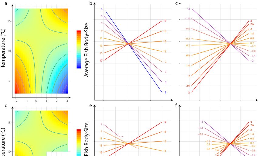
of eutrophication. At low temperatures (13 °C) (Figure 3e) and a decrease in body size
temperature for low levels of eutrophication (Figure 3f). Compared with Figure 3a, the amplitude
with temperature for low levels of eutrophication (Figure 3f). Compared with Figure 3a, the
amplitude of body size in response to pressure conditions was reduced. The lowest values associatedWater 2020, 12, 779 9 of 17
Water 2020,size
of body 12, 779
in 9 ofan
response to pressure conditions was reduced. The lowest values associated with 16
increase in temperature at low eutrophication were not observed with the observed pressure values
with an increase in temperature at low eutrophication were not observed with the observed pressure
(Figure 3d).
values (Figure 3d).
Figure 3. Effect of interaction between average temperature and eutrophication level on Average Fish
Figure 3. Effect of interaction between average temperature and eutrophication level on Average Fish
Body Size when considering all possible combinations of pressures (a–c), or when considering only the
Body Size when considering all possible combinations of pressures (a–c), or when considering only
observed combination of pressures (see Figure 1) (d–f). (a,d) Low theoretical values are in blue and
the observed combination of pressures (see Figure 1) (d–f). (a,d) Low theoretical values are in blue
high theoretical values in red.
and high theoretical values in red.
4. Discussion
4. Discussion
The objective of our study was to assess the interactive effect of temperature and eutrophication
on theThe objective
structure of of our
fish study
and was to assess
phytoplankton the interactive
communities. effect the
Among of temperature and eutrophication
twelve pressure/impact models
on the structure of fish and phytoplankton communities. Among the twelve
developed, an additive effect and an interactive effect were detected for, respectively one and two fish pressure/impact models
developed,
metrics, while an most
additive of theeffect and reveal
models an interactive effect
a significant wereofdetected
effect for, respectively one and two
one stressor.
fish metrics,
The impactwhile most of the models
of eutrophication reveal a communities
on biological significant effect of one
has long beenstressor.
observed [41]. For example,
the effects of phosphorus loadings on primary production have largely been been
The impact of eutrophication on biological communities has long observed
described in the [41]. For
scientific
example, the effects of phosphorus loadings on primary production have
literature [80–82]. Algal blooms in response to eutrophication are also well-documented [83], as well largely been described in
the scientific
as the changes literature
in community [80–82].structure
Algal blooms in responseThe
[34,42,66,84,85]. to eutrophication
impact of temperatureare also has
well-documented
been explored
[83], as well as the changes in community structure [34,42,66,84,85]. The impact
in detail, and is often still studied, especially since climate change has become evident [86]. The effect of temperature has
been
of anexplored
increase in indetail, and is often
temperature couldstill
bestudied,
manifold especially since climate
and complex (see, for change has become
instance, evident
Keller [87] and
[86]. The effect of an increase in temperature could be manifold and complex (see,
Richardson et al. [19]), but many authors agree on an increase in productivity [38,88,89] or on a decrease for instance, Keller
[87] and Richardson
in ectothermal et al. [19]),Most
size [57,90,91]. but many
of ourauthors
resultsagree
are inon an increase
accordance in productivity
with [38,88,89]
these observations. or
Fish
on a decrease
density expressed in inectothermal size [57,90,91].
occurrence (CPUE) was shown Most of positively
to be our results are in accordance
correlated with an increasewithinthese
both
observations. Fish density expressed in occurrence (CPUE) was shown
temperature and eutrophication. Similarly, the biomass of fish per capture effort (BPUE) and Chl-a to be positively correlated
with an
were increaserelated
positively in both to temperature and eutrophication.
nutrient enrichment. This increasing Similarly, the biomass
productivity of fish per and
of phytoplankton capture
fish
efforteutrophication
with (BPUE) and Chl-a were positively
[36,38,92] is generallyrelated to nutrient
associated with enrichment. This increasing
the shift in community productivity
composition and
of phytoplankton
structure [35], which and is fish with eutrophication
also observed in our case,[36,38,92]
through the is generally
ratio of perchassociated
vs. roachwith the shiftand
biomasses in
community
Chrysophytes composition
biomass. The andbiomass
structureof[35], which is also
Chrysophytes wasobserved
shown to indecrease
our case,when through the ratio of
eutrophication
perch vs. roach biomasses and Chrysophytes biomass. The biomass
increases, which is consistent with our hypothesis and previous results [34,35,85]. of Chrysophytes was shown to
decrease when eutrophication increases, which is consistent with our hypothesis
Of the two metrics related to CSS, slope and midpoints, only the latter was shown to increase and previous results
[34,35,85].
with eutrophication. Finally, four metrics for which response to eutrophication and/or temperature
Of the two were
were expected, metrics notrelated
explainedto CSS,
by ourslope and midpoints,
models: CSS_Slope, only the latter wasSize
Phytoplankton shown to Average
Class, increase
with eutrophication. Finally, four metrics for which response to eutrophication and/or temperature
were expected, were not explained by our models: CSS_Slope, Phytoplankton Size Class, Average
Perch/Roach Body Size, and Cyano_Biovolume. The absence of impact of the stressors can beWater 2020, 12, 779 10 of 17
Perch/Roach Body Size, and Cyano_Biovolume. The absence of impact of the stressors can be attributed
to sampling protocol (reduction of the size range variability by gillnet selectivity for fish) and to size
assessment for phytoplankton (very simplified and coarse) [41,42,66]. In addition, the high temporal
and spatial variability of the abundance of cyanobacteria is a limit to this type of analysis [93,94].
In addition to the effect of pressures, we saw the significant proportion of model variability
explained by the environmental characteristics of lakes confirming previous results and patterns when
focusing on pressures [67,68].
More interestingly, two metrics were sensitive to the interaction of temperature and eutrophication:
BPUE ratio between perch and roach and average community size. The interaction of these two
pressures on the BPUE ratio between perch and roach highlighted the role played by temperature
on the magnitude of this relationship. This was even more evident when graph effect displays were
represented only on the observed range of values of these pressures (Figure 2d–f). The slope of the
relation between eutrophication and BPUE ratio increased as the temperature increased (especially
between 12 and 16 degrees). When all possible combinations of the pressures (Figure 2a–c) are used
to visualize the estimated effect of each pressure (taking into account the second pressure due to
the interaction between the two), some unexpected relationship may appear: for instance, a positive
relationship between the ratio of perch/roach biomasses and nutrient enrichment for cold lakes
(see Figure 2b). This is probably due to deep extrapolations for non-observed pressure conditions.
Unlike an experimental design, for which environmental conditions are controlled and a perfect
crossover of pressures can be used, the cold lakes in our dataset were mainly oligotrophic. Eutrophic
lakes were predominantly observed under cool and warm conditions (Figure 1). However, interactive
effects of temperature and nutrients on community dynamics are very often studied and observed on
phytoplankton [37,84,85], but poorly tested for fish.
The relationship between fish size and temperature has been well studied, especially in the context
of global warming (e.g., [57]). The significant interaction between eutrophication and temperature
suggested that the magnitude as well as the sign of the relationship between temperature and average
community size depends on trophic level. In oligotrophic conditions, community size was estimated
to decrease along thermal gradients. This pattern has already been observed for fish [57,91], especially
in lakes [95]. Ectothermal individuals could be smaller in warmer conditions, according to the
temperature size rule theory [90], and/or smaller species could be preferentially selected as temperature
increases [57,91]. With nutrient enrichment, the model predicted that average community size would
increase with temperature, which is contradictory to the theory prediction. Nonetheless, fish in
fisheries would grow faster and larger when the temperature increases, but when they are fed ad
libitum [96]. This could also be explained by a more efficient trophic transfer and more available
resources amplified through the trophic level with warming, as predicted by metabolic theory in
nutrient-replete systems [97].
The fact that some components of community structure are impacted by different pressures and, in
particular, their interaction should provide water managers with strong insight. Until recently in Europe,
water managers mainly focused on pressure—impact relationships through multi-metric indices [98,99]
to assess the ecological status of lakes [100,101] owing to the WFD. Such interaction could influence
the scoring values of metrics, then metric index values and ecological assessment, but Miguet et al. [28]
evaluated it at a small deviation. More recently, rather than focusing on ecological status, which is a
current evaluation, some authors have worked on the vulnerability of lake ecosystems (e.g., [102]).
This concept was designed around three components—sensitivity (the degree to which communities
are affected, either adversely or beneficially, by pressure), exposure (contact between communities
and stressors) and capacity to adapt (the ability of communities to adjust to potential hazards, to take
advantage of opportunities or to respond to consequences) [103]—and seems very interesting for
anticipating/forecasting lakes that will suffer from global warming. Addressing the vulnerability of
communities to multiple stressors appears necessary in order to prevent future alterations in aquatic
ecosystems by prioritizing the protection of the most vulnerable structures [104,105]. Our study showsWater 2020, 12, 779 11 of 17
that the sensitivity of communities is modulated both by the level of exposure to pressures and by the
coupling of these pressures. If the interaction of pressures is seen as an additive effect, while multiple
interactions could occur [7], then the sensitivity of the communities might be inconsistently evaluated,
since the actual effect of a pressure would be related to the level of the other pressures. Thus, by
ignoring interaction, there is a risk of an unexpected ecological effect by underestimating the effect of
pressure, or even concluding that an effect in the opposite direction depends on the exposure level to
another pressure [5,6]. This could lead to the adoption of an inappropriate strategy to manage lakes or
to not prioritizing management actions for lakes that could actually be much more vulnerable than
expected. With the increase of stress on freshwater ecosystems such as lakes, it will be necessary to
pursue our monitoring on these systems to study their combined effects with global change and how
this will impact aquatic communities [7,106].
To conclude, we highlight in situ interactive effects of eutrophication and temperature on lake fish
communities. Therefore, in light of these unexpected effects, future management plans should consider
the type and strength of interactions in order to avoid underestimating the vulnerability of these
environments [105,107]. Finally, a consideration of pressure interaction in the study of environmental
vulnerability could help to identify priorities for action to conserve and restore aquatic environments.
Supplementary Materials: The following are available online at http://www.mdpi.com/2073-4441/12/3/779/s1,
Table S1: Linear Model Coefficients of biological metrics, Table S2: Environmental characteristic of the 204 lakes in
the dataset.
Author Contributions: Conceptualization, investigation, draft preparation, by L.B., M.L, C.L.-T., and C.A.;
methodology, formal analysis by L.B. and M.L. All authors have read and agreed to the published version of
the manuscript.
Funding: This research was funded by the Research & Development center “ECLA” and by the South Region
(Provence-Alpes-Côte d’Azur) grant number n 2018-05953.
Acknowledgments: The authors are grateful to all those who participated in data collection and management,
especially Nathalie Reynaud, Thierry Point, and Thierry Tormos. The authors also thank Pierre Alain Danis for his
valuable help with temperature data, Paul Miguet for his advice and for English correction, Isabella Athanassiou
and Eric Hernquist.
Conflicts of Interest: The authors declare no conflict of interest.
References
1. Dudgeon, D.; Arthington, A.H.; Gessner, M.O.; Kawabata, Z.-I.; Knowler, D.J.; Lévêque, C.; Naiman, R.J.;
Prieur-Richard, A.-H.; Soto, D.; Stiassny, M.L.J.; et al. Freshwater biodiversity: Importance, threats, status
and conservation challenges. Biol. Rev. 2006, 81, 163. [CrossRef]
2. Lundberg, J.G.; Kottelat, M.; Smith, G.R.; Stiassny, M.L.J.; Gill, A.C. So Many Fishes, So Little Time: An
Overview of Recent Ichthyological Discovery in Continental Waters. Ann. Mo. Bot. Gard. 2000, 87, 26.
[CrossRef]
3. Sala, O.E. Global Biodiversity Scenarios for the Year 2100. Science 2000, 287, 1770–1774. [CrossRef]
4. Hering, D.; Carvalho, L.; Argillier, C.; Beklioglu, M.; Borja, A.; Cardoso, A.C.; Duel, H.; Ferreira, T.;
Globevnik, L.; Hanganu, J.; et al. Managing aquatic ecosystems and water resources under multiple stress
—An introduction to the MARS project. Sci. Total Environ. 2015, 503–504, 10–21. [CrossRef]
5. Jackson, M.C.; Woodford, D.J.; Weyl, O.L.F. Linking key environmental stressors with the delivery of
provisioning ecosystem services in the freshwaters of southern Africa: Environmental stress and ecosystem
services. Geo Geogr. Environ. 2016, 3, e00026. [CrossRef]
6. Ormerod, S.J.; Dobson, M.; Hildrew, A.G.; Townsend, C.R. Multiple stressors in freshwater ecosystems.
Freshw. Biol. 2010, 55, 1–4. [CrossRef]
7. Schinegger, R.; Palt, M.; Segurado, P.; Schmutz, S. Untangling the effects of multiple human stressors and
their impacts on fish assemblages in European running waters. Sci. Total Environ. 2016, 573, 1079–1088.
[CrossRef] [PubMed]
8. Wagner, T.; Erickson, L.E. Sustainable Management of Eutrophic Lakes and Reservoirs. J. Environ. Prot. 2017,
8, 436–463. [CrossRef]Water 2020, 12, 779 12 of 17
9. Côté, I.M.; Darling, E.S.; Brown, C.J. Interactions among ecosystem stressors and their importance in
conservation. Proc. R. Soc. B Biol. Sci. 2016, 283, 20152592. [CrossRef] [PubMed]
10. Nõges, P.; Argillier, C.; Borja, Á.; Garmendia, J.M.; Hanganu, J.; Kodeš, V.; Pletterbauer, F.; Sagouis, A.;
Birk, S. Quantified biotic and abiotic responses to multiple stress in freshwater, marine and ground waters.
Sci. Total Environ. 2016, 540, 43–52. [CrossRef]
11. Poikane, S.; Ritterbusch, D.; Argillier, C.; Białokoz, W.; Blabolil, P.; Breine, J.; Jaarsma, N.G.; Krause, T.;
Kubečka, J.; Lauridsen, T.L.; et al. Response of fish communities to multiple pressures: Development of a
total anthropogenic pressure intensity index. Sci. Total Environ. 2017, 586, 502–511. [CrossRef] [PubMed]
12. Kristensen, P.; Whalley, C.; Zal, F.; Christiansen, T.; Schmedtje, U.; Solheim, A.; Austnes, K.; Kampa, E.;
Rouillard, J.; Prchalova, H.; et al. 2018 EEA European Waters Assessment; European Waters Assessment; Office
for Official Publications of the European Union: Copenhagen, Denmark, 2018; Volume 7.
13. Kristensen, P.; Vanneuville, W. Climate Change, Impacts and Vulnerability in Europe 2012: An Indicator-Based Report
Section 3.3: Freshwater Quantity and Quality; European Waters Assessment; Office for Official Publications of
the European Union: Luxembourg, 2012; Volume 12, pp. 119–127.
14. Chen, X.; Yang, X.; Dong, X.; Liu, E. Environmental changes in Chaohu Lake (southeast, China) since the
mid 20th century: The interactive impacts of nutrients, hydrology and climate. Limnologica 2013, 43, 10–17.
[CrossRef]
15. Salmaso, N. Interactions between nutrient availability and climatic fluctuations as determinants of the
long-term phytoplankton community changes in Lake Garda, Northern Italy. Hydrobiologia 2011, 660, 59–68.
[CrossRef]
16. Scheffer, M.; van Nes, E.H. Shallow lakes theory revisited: Various alternative regimes driven by climate,
nutrients, depth and lake size. Hydrobiologia 2007, 584, 455–466. [CrossRef]
17. Shurin, J.B.; Winder, M.; Adrian, R.; Keller, W.; Matthews, B.; Paterson, A.M.; Paterson, M.J.; Pinel-Alloul, B.;
Rusak, J.A.; Yan, N.D. Environmental stability and lake zooplankton diversity—Contrasting effects of
chemical and thermal variability. Ecol. Lett. 2010, 13, 453–463. [CrossRef]
18. Kosten, S.; Huszar, V.L.M.; Bécares, E.; Costa, L.S.; Donk, E.; Hansson, L.-A.; Jeppesen, E.; Kruk, C.; Lacerot, G.;
Mazzeo, N.; et al. Warmer climates boost cyanobacterial dominance in shallow lakes. Glob. Chang. Biol.
2012, 18, 118–126. [CrossRef]
19. Richardson, J.; Miller, C.; Maberly, S.C.; Taylor, P.; Globevnik, L.; Hunter, P.; Jeppesen, E.; Mischke, U.;
Moe, S.J.; Pasztaleniec, A.; et al. Effects of multiple stressors on cyanobacteria abundance vary with lake
type. Glob. Chang. Biol. 2018, 24, 5044–5055. [CrossRef]
20. Jeppesen, E.; Mehner, T.; Winfield, I.J.; Kangur, K.; Sarvala, J.; Gerdeaux, D.; Rask, M.; Malmquist, H.J.;
Holmgren, K.; Volta, P.; et al. Impacts of climate warming on the long-term dynamics of key fish species in
24 European lakes. Hydrobiologia 2012, 694, 1–39. [CrossRef]
21. Crain, C.M.; Kroeker, K.; Halpern, B.S. Interactive and cumulative effects of multiple human stressors in
marine systems. Ecol. Lett. 2008, 11, 1304–1315. [CrossRef]
22. Piggott, J.J.; Townsend, C.R.; Matthaei, C.D. Reconceptualizing synergism and antagonism among multiple
stressors. Ecol. Evol. 2015, 5, 1538–1547. [CrossRef] [PubMed]
23. Folt, C.L.; Chen, C.Y.; Moore, M.V.; Burnaford, J. Synergism and antagonism among multiple stressors.
Limnol. Oceanogr. 1999, 44, 864–877. [CrossRef]
24. Rigosi, A.; Carey, C.C.; Ibelings, B.W.; Brookes, J.D. The interaction between climate warming
and eutrophication to promote cyanobacteria is dependent on trophic state and varies among taxa.
Limnol. Oceanogr. 2014, 59, 99–114. [CrossRef]
25. Matthaei, C.D.; Piggott, J.J.; Townsend, C.R. Multiple stressors in agricultural streams: Interactions among
sediment addition, nutrient enrichment and water abstraction: Sediment, nutrients & water abstraction.
J. Appl. Ecol. 2010, 47, 639–649.
26. Piggott, J.J.; Lange, K.; Townsend, C.R.; Matthaei, C.D. Multiple Stressors in Agricultural Streams:
A Mesocosm Study of Interactions among Raised Water Temperature, Sediment Addition and Nutrient
Enrichment. PLoS ONE 2012, 7, e49873. [CrossRef] [PubMed]
27. Townsend, C.R.; Uhlmann, S.S.; Matthaei, C.D. Individual and combined responses of stream ecosystems to
multiple stressors. J. Appl. Ecol. 2008, 45, 1810–1819. [CrossRef]Water 2020, 12, 779 13 of 17
28. Miguet, P.; Logez, M.; Argillier, C. Incertitudes Liées aux Interactions de Pressions. Effet des Interactions Entre les
Pressions sur les Métriques Constitutives des Indicateurs IIL et IIR—Rapport AQUAREF. Personal Communication;
Irstea: Aix-en-provence, France, 2018.
29. Paine, R.T.; Tegner, M.J.; Johnson, E.A. Compounded Perturbations Yield Ecological Surprises. Ecosystems
1998, 1, 535–545. [CrossRef]
30. Villar-Argaiz, M.; Medina-Sánchez, J.M.; Biddanda, B.A.; Carrillo, P. Predominant Non-additive Effects
of Multiple Stressors on Autotroph C:N:P Ratios Propagate in Freshwater and Marine Food Webs.
Front. Microbiol. 2018, 9, 69. [CrossRef]
31. Lange, K.; Townsend, C.R.; Matthaei, C.D. Inconsistent Relationships of Primary Consumer N Stable Isotope
Values to Gradients of Sheep/Beef Farming Intensity and Flow Reduction in Streams. Water 2019, 11, 2239.
[CrossRef]
32. Walters, A.W.; Bartz, K.K.; Mcclure, M.M. Interactive Effects of Water Diversion and Climate Change
for Juvenile Chinook Salmon in the Lemhi River Basin (U.S.A.): Water Diversion and Climate Change.
Conserv. Biol. 2013, 27, 1179–1189. [CrossRef]
33. Wenger, S.J.; Isaak, D.J.; Luce, C.H.; Neville, H.M.; Fausch, K.D.; Dunham, J.B.; Dauwalter, D.C.; Young, M.K.;
Elsner, M.M.; Rieman, B.E.; et al. Flow regime, temperature, and biotic interactions drive differential declines
of trout species under climate change. Proc. Natl. Acad. Sci. USA 2011, 108, 14175–14180. [CrossRef]
34. Winder, M.; Reuter, J.E.; Schladow, S.G. Lake warming favours small-sized planktonic diatom species. Proc. R.
Soc. B Biol. Sci. 2009, 276, 427–435. [CrossRef]
35. Jeppesen, E.; Sondergaard, M.; Jensen, J.P.; Havens, K.E.; Anneville, O.; Carvalho, L.; Coveney, M.F.;
Deneke, R.; Dokulil, M.T.; Foy, B.; et al. Lake responses to reduced nutrient loading—An analysis of
contemporary long-term data from 35 case studies. Freshw. Biol. 2005, 50, 1747–1771. [CrossRef]
36. Jeppesen, E.; Peder Jensen, J.; SØndergaard, M.; Lauridsen, T.; Landkildehus, F. Trophic structure, species
richness and biodiversity in Danish lakes: Changes along a phosphorus gradient: A detailed study of Danish
lakes along a phosphorus gradient. Freshw. Biol. 2000, 45, 201–218. [CrossRef]
37. Kratina, P.; Greig, H.S.; Thompson, P.L.; Carvalho-Pereira, T.S.A.; Shurin, J.B. Warming modifies trophic
cascades and eutrophication in experimental freshwater communities. Ecology 2012, 93, 1421–1430. [CrossRef]
[PubMed]
38. Bucak, T.; Saraoğlu, E.; Levi, E.E.; Nihan Tavşanoğlu, Ü.; İdİl Çakiroğlu, A.; Jeppesen, E.; Beklioğlu, M.
The influence of water level on macrophyte growth and trophic interactions in eutrophic Mediterranean
shallow lakes: A mesocosm experiment with and without fish: Effects of water level in warm shallow lakes.
Freshw. Biol. 2012, 57, 1631–1642. [CrossRef]
39. Downing, J.A.; Plante, C.; Lalonde, S. Fish Production Correlated with Primary Productivity, not the
Morphoedaphic Index. Can. J. Fish. Aquat. Sci. 1990, 47, 1929–1936. [CrossRef]
40. Kronvang, B.; Jeppesen, E.; Conley, D.J.; Søndergaard, M.; Larsen, S.E.; Ovesen, N.B.; Carstensen, J. Nutrient
pressures and ecological responses to nutrient loading reductions in Danish streams, lakes and coastal waters.
J. Hydrol. 2005, 304, 274–288. [CrossRef]
41. Meerhoff, M.; Teixeira-de Mello, F.; Kruk, C.; Alonso, C.; González-Bergonzoni, I.; Pacheco, J.P.; Lacerot, G.;
Arim, M.; Beklioğlu, M.; Brucet, S.; et al. Environmental Warming in Shallow Lakes. In Advances in Ecological
Research; Elsevier: London, UK, 2012; Volume 46, pp. 259–349.
42. Moss, B.; Stephen, D.; Balayla, D.M.; Becares, E.; Collings, S.E.; Fernandez-Alaez, C.; Fernandez-Alaez, M.;
Ferriol, C.; Garcia, P.; Goma, J.; et al. Continental-scale patterns of nutrient and fish effects on shallow lakes:
Synthesis of a pan-European mesocosm experiment. Freshw. Biol. 2004, 49, 1633–1649. [CrossRef]
43. Persson, L.; Diehl, S.; Johansson, L.; Andersson, G.; Hamrin, S.F. Shifts in fish communities along the
productivity gradient of temperate lakes-patterns and the importance of size-structured interactions.
J. Fish Biol. 1991, 38, 281–293. [CrossRef]
44. European Committee for Standardization (CEN). Water Quality—Guidance on the Scope and Selection of Fish
Sampling Methods (English Version EN 14757:2015); European Committee for Standardization; BSI Standards:
Brussels, Belgium, 2015.
45. Prchalová, M.; Mrkvička, T.; Kubečka, J.; Peterka, J.; Čech, M.; Muška, M.; Kratochvíl, M.; Vašek, M. Fish
activity as determined by gillnet catch: A comparison of two reservoirs of different turbidity. Fish. Res. 2010,
102, 291–296. [CrossRef]Water 2020, 12, 779 14 of 17
46. Šmejkal, M.; Ricard, D.; Prchalová, M.; Říha, M.; Muška, M.; Blabolil, P.; Čech, M.; Vašek, M.; Jůza, T.;
Monteoliva Herreras, A.; et al. Biomass and Abundance Biases in European Standard Gillnet Sampling.
PLoS ONE 2015, 10, e0122437. [CrossRef] [PubMed]
47. Laplace-Treyture, C.; Rimet, F.; Anneville, O.; Druart, J.-C.; Barbe, J.; Dutartre, A. Protocole Standardisé
D’échantillonnage, de Conservation, D’observation et de Dénombrement du Phytoplancton en Plan D’eau Pour la
Mise en Œuvre de la DCE: Version 3.3.1. Personal Communication; Cemagref: Cestas, France, 2009; p. 44.
48. CEN-EN 15204. Water Quality. Guidance Standard on the Enumeration of Phytoplankton Using Inverted Microscopy
(Utermöhl Technique); AFNOR Normalisation: La plaine Saint-Denis, France, 2006; p. 39.
49. Derot, J.; Jamoneau, A.; Teichert, N.; Rosebery, J.; Morin, S.; Laplace-Treyture, C. Response of phytoplankton
traits to environmental variables in French lakes: New perspectives for bioindication. Ecol. Indic. 2020, 108,
105659. [CrossRef]
50. Laplace-Treyture, C.; Hadoux, E.; Plaire, M.; Dubertrand, A.; Esmieu, P. PHYTOBS v3.0: Outil de Comptage
du Phytoplancton en Laboratoire et de Calcul de l’IPLAC. Version 3.0. Application JAVA. Personal Communication;
Irstea: Cestas, France, 2017.
51. Laplace-Treyture, C.; Feret, T. Performance of the Phytoplankton Index for Lakes (IPLAC): A multimetric
phytoplankton index to assess the ecological status of water bodies in France. Ecol. Indic. 2016, 69, 686–698.
[CrossRef]
52. CEN-EN 90-117. Water Quality—Determination of Chlorophyll a and of a Pheopigments Index. Molecular Absorption
Spectrometric Method; AFNOR Normalisation: Paris, France, 1999; p. 11.
53. Bergström, L.; Karlsson, M.; Bergström, U.; Pihl, L.; Kraufvelin, P. Relative impacts of fishing and
eutrophication on coastal fish assessed by comparing a no-take area with an environmental gradient.
Ambio 2019, 48, 565–579. [CrossRef]
54. Van Dorst, R.M.; Gårdmark, A.; Svanbäck, R.; Beier, U.; Weyhenmeyer, G.A.; Huss, M. Warmer and browner
waters decrease fish biomass production. Glob. Chang. Biol. 2019, 25, 1395–1408. [CrossRef]
55. Deceliere-Vergès, C.; Argillier, C.; Lanoiselée, C.; De Bortoli, J.; Guillard, J. Stability and precision of the fish
metrics obtained using CEN multi-mesh gillnets in natural and artificial lakes in France. Fish. Res. 2009, 99,
17–25. [CrossRef]
56. Irz, P.; Odion, M.; Argillier, C.; Pont, D. Comparison between the fish communities of lakes, reservoirs and
rivers: Can natural systems help define the ecological potential of reservoirs? Aquat. Sci. 2006, 68, 109–116.
[CrossRef]
57. Daufresne, M.; Lengfellner, K.; Sommer, U. Global warming benefits the small in aquatic ecosystems.
Proc. Natl. Acad. Sci. USA 2009, 106, 12788–12793. [CrossRef]
58. Ohlberger, J. Climate warming and ectotherm body size—From individual physiology to community ecology.
Funct. Ecol. 2013, 27, 991–1001. [CrossRef]
59. White, E.P.; Ernest, S.K.M.; Kerkhoff, A.J.; Enquist, B.J. Relationships between body size and abundance in
ecology. Trends Ecol. Evol. 2007, 22, 323–330. [CrossRef]
60. Guiet, J.; Poggiale, J.-C.; Maury, O. Modelling the community size-spectrum: Recent developments and new
directions. Ecol. Model. 2016, 337, 4–14. [CrossRef]
61. Bartosiewicz, M.; Przytulska, A.; Deshpande, B.N.; Antoniades, D.; Cortes, A.; MacIntyre, S.; Lehmann, M.F.;
Laurion, I. Effects of climate change and episodic heat events on cyanobacteria in a eutrophic polymictic lake.
Sci. Total Environ. 2019, 693, 133414. [CrossRef] [PubMed]
62. Korkonen, S.; Weckström, J.; Korhola, A. Biogeography and ecology of freshwater chrysophyte cysts in
Finland. Hydrobiologia 2019, 847, 497–499. [CrossRef]
63. Moss, B.; Kosten, S.; Meerhoff, M.; Battarbee, R.W.; Jeppesen, E.; Mazzeo, N.; Havens, K.; Lacerot, G.; Liu, Z.;
De Meester, L.; et al. Allied attack: Climate change and eutrophication. Inland Waters 2011, 1, 101–105.
[CrossRef]
64. Ignatiades, L. Redefinition of cell size classification of phytoplankton—A potential tool for improving the
quality and assurance of data interpretation. Mediterr. Mar. Sci. 2015, 17, 56. [CrossRef]
65. Kruk, C.; Huszar, V.L.M.; Peeters, E.T.H.M.; Bonilla, S.; Costa, L.; LüRling, M.; Reynolds, C.S.; Scheffer, M.
A morphological classification capturing functional variation in phytoplankton. Freshw. Biol. 2010, 55,
614–627. [CrossRef]You can also read