A new Hybrid Radiative Transfer Method for Massive Star Formation
←
→
Page content transcription
If your browser does not render page correctly, please read the page content below
Astronomy & Astrophysics manuscript no. output                                                                                         c ESO 2020
January 14, 2020

           A new Hybrid Radiative Transfer Method for Massive Star
                                 Formation
                                R. Mignon-Risse1 , M. González1 , B. Commerçon2 , and J. Rosdahl3

      1
          AIM, CEA, CNRS, Université Paris-Saclay, Université Paris Diderot, Sorbonne Paris Cité, F-91191 Gif-sur-Yvette, France
          e-mail: raphael.mignon-risse@cea.fr
      2
          Centre de Recherche Astrophysique de Lyon UMR5574, ENS de Lyon, Univ. Lyon1, CNRS, Université de Lyon, 69007 Lyon,
          France
      3
          Univ Lyon, Univ Lyon1, Ens de Lyon, CNRS, Centre de Recherche Astrophysique de Lyon UMR5574, F-69230, Saint-Genis-
          Laval, France

      Received ?; ?

                                                                    ABSTRACT

      Context. Frequency-dependent and/or hybrid approaches for the treatment of stellar irradiation are of primary importance in numerical
      simulations of massive star formation.
      Aims. We seek to compare outflow and accretion mechanisms in star formation simulations. We investigate the accuracy of a hybrid
      radiative transfer method using the gray M1 closure relation for proto-stellar irradiation and gray Flux-Limited Diffusion (FLD) for
      photons emitted everywhere else.
      Methods. We have coupled the FLD module of the adaptive-mesh refinement code Ramses with Ramses-RT, which is based on the
      M1 closure relation and the reduced speed-of-light-approximation. Our hybrid (M1+FLD) method takes an average opacity at the
      stellar temperature for the M1 module, instead of the local environmental radiation field. By construction, the opacities are consistent
      with the photon origin. We have tested this approach in radiative transfer tests of disks irradiated by a star for three levels of optical
      thickness and compared the temperature structure with the radiative transfer codes RADMC-3D and MCFOST. We apply it to a
      radiation-hydrodynamical simulation of massive star formation.
      Results. Our tests validate our hybrid approach for determining the temperature structure of an irradiated disk in the optically-thin (2%
      maximal error) and moderately optically-thick (error smaller than 25%) regimes. The most optically-thick test shows the limitation
      of our hybrid approach with a maximal error of 76% in the disk mid-plane against 94% with the FLD method. The optically-thick
      setups highlight the hybrid method ability to capture partially the self-shielding in the disk while the FLD alone cannot. The radiative
      acceleration is ≈100 times greater with the hybrid method than with the FLD. Consistently, the hybrid method leads to about +50%
      more extended and wider-angle radiative outflows in the massive star formation simulation. We obtain a 17.6 M star at t'0.7τff , while
      the accretion phase is still ongoing, with a mean accretion rate of '7 × 10⁻⁴ M yr−1 . Finally, despite the use of refinement to resolve
      the radiative cavities, no Rayleigh-Taylor instability appears in our simulations, and we justify their absence by physical arguments
      based on the entropy gradient.
      Key words. Stars: formation – Stars: massive – Stars: protostars – Radiative transfer – Hydrodynamics – Methods: numerical

1. Introduction                                                             tationally collapses while fragmentation is limited by turbulent,
                                                                            radiative and magnetic support (e.g. Commerçon et al. 2011a).
Massive stars shape the dynamical and chemical evolution of                 The IMF is therefore linked to the prestellar core mass func-
galaxies because of their powerful feedback in radiation, winds,            tion, as more massive stars form in more massive cores. For re-
explosions in supernova and metal-enrichment, however their                 views on theories of massive star formation, we refer the reader
formation remains a long-standing problem. Observationally,                 to Beuther et al. (2007), Zinnecker & Yorke (2007), Tan et al.
massive stars are embedded in dense clouds, they form on                    (2014), Krumholz (2017).
timescales much shorter than their low-mass counterpart (Motte                  There is no consensus regarding the accretion process, and a
et al. 2007) and are likely to be located at distances larger than          way to probe it is to study outflows. Indeed, magnetic outflows
1 kpc from us, which makes their formation process challeng-                are often associated with accretion (Blandford & Payne 1982,
ing to observe. Two major scenarios are under active studies:               Pelletier & Pudritz 1992), as they remove the angular momen-
the competitive accretion model and the turbulent core accre-               tum from an accretion disk, and they do not require strong mag-
tion model. In the competitive accretion model (Bonnell et al.              netic fields. It is then possible to study the physics of accretion
2004), all stars form in clusters and stars located at the center of        via the outflow properties (Pudritz et al. 2006), and in particular
the gravitational potential will gain more mass and will eventu-            the accretion rate from the outflow velocity (Pelletier & Pudritz
ally become massive stars, via accretion and possibly merging               1992). In the case of massive stars, they can act as a channel for
processes. In this scenario, the Initial-Mass Function (IMF) is             the radiation to escape. Moreover, accretion modes differ from
built-up naturally. On the other hand, the turbulent core model             one scenario to another. Disk accretion is more likely to occur
(McKee & Tan 2003) is an extension of the low-mass star for-                in the turbulent core accretion model, with high accretion rates
mation scenario. A massive and turbulent prestellar core gravi-             (Ṁ∼10−4 −10−3 M yr−1 , McKee & Tan 2003). More chaotic ac-
                                                                                                                        Article number, page 1 of 17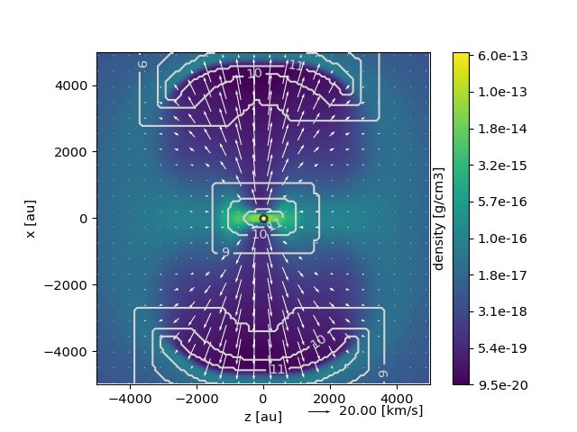
A&A proofs: manuscript no. output

cretion mechanisms are associated with the competitive accre-            also noted the formation of polar cavities dominated by the stel-
tion model or with models including accretion via filaments. Re-         lar radiative pressure, enhanced by the particular treatment of
cent observations by Goddi et al. (2018) reveal signatures of out-       stellar irradiation.
flows whose direction varies through time. If they are perpendic-             In addition, Krumholz et al. (2009) and Rosen et al. (2016)
ular to the accretion disk (Blandford & Payne 1982), this indi-          observe the onset of radiative Rayleigh-Taylor instabilities in the
cates that the plane of accretion changes with time, favouring ac-       radiation-pressure-dominated cavities that feed the star-disk sys-
cretion via filaments and competitive accretion. The study of out-       tem and help accreting mass onto the central star via the flash-
flows can indeed help to distinguishing the accretion modes, and         light effect. However, these instabilities have not been observed
these questions highlight the need for realistic outflow models          in the work of Kuiper et al. (2010a) and Klassen et al. (2016).
(magnetic and/or radiative) in numerical simulations. Regarding          Kuiper et al. (2012) argue that a gray FLD model, as used in
the radiative outflows, this means the use of a radiative transport      Krumholz et al. (2009), underestimates the radiation force in the
method well-suited in the optically-thin regime. Current and past        cavity and can artificially lead to the apparition of these instabil-
studies of massive star formation have mainly focused on its ra-         ities. With a frequency-dependent hybrid model and a Cartesian
diative aspects. In a 1D spherically-symmetric approach, the ra-         grid, Klassen et al. (2016) did not obtain such instabilities while
diative force of a massive (proto)star is expected to counteract         Rosen et al. (2016) did. The difference in their results can be ex-
gravity up to the point where accretion is stopped, as computed          plained by the use of refinement by Rosen et al. (2016) to resolve
analytically (Larson & Starrfield 1971) and then numerically             the seeds of the instabilities, the smallest modes being the more
(Kuiper et al. 2010a). Their results showed that the highest mass        unstable (Jacquet & Krumholz 2011). Contrarily, the spherical
reached was 40 M . 2D and 3D numerical simulations have per-             grid without additional refinement in the cavities used by Kuiper
mitted the emergence of a new accretion mode, the flashlight             et al. (2012) would not permit to refine them. It is thus unclear
effect (Yorke & Sonnhalter 2002), which allows the radiation to          yet whether this mechanism is at work during the formation of
escape freely in the poles while material is accreted through the        massive stars. Meanwhile, it is clear that disk-accretion is suffi-
disk (Krumholz et al. 2009, Kuiper et al. 2010a, Rosen et al.            cient to reach masses consistent with the massive stars observed.
2016, Harries et al. 2017).                                              Our hybrid method, implemented in the Cartesian adaptive-mesh
    Monte-Carlo approaches are often used for solving radiative          refinement (AMR) code Ramses (Teyssier 2002) will help us to
transfer problems for their accuracy but they are particularly ex-       establish the importance of these accretion mechanisms, by cap-
pensive and their computational time scales with the number              turing the non-isotropy of the radiation field.
of radiative sources. This justifies the use of fluid description             This paper is organized as follows. Section 2 presents the
models, such as the Flux-Limited Diffusion (FLD) and the M1              equations of the Flux-Limited Diffusion method and the M1
methods, for Radiation-HydroDynamics (RHD). The first RHD                method, along with their coupling and implementation in the
calculations relied on the Flux-Limited Diffusion (FLD) closure          Ramses code. We present the tests and the validation of our hy-
relation for its simplicity and advantageous computational cost.         brid approach in Section 3 and its application to the collapse of
However, it is more suited for the optically-thick regime, while         a massive prestellar core leading to the formation of a massive
the use of a flux-limiter corrects the propagation speed in the          star in Section 4. We discuss our results in Section 5
optically-thin regime (Levermore & Pomraning 1981). In addi-
tion, the FLD method does not permit to capture shadows behind
very optically-thick gas. In the context of massive star formation,      2. Methods
the flashlight effect is due to the non-isotropic character of the ra-   In this section, we present the equations of the hybrid radiative
diation field because the optical thickness is very different in the     transfer approach and its implementation: the M1 method for the
disk direction and in the cavities direction. Therefore, numerical       stellar irradiation and the Flux-Limited Diffusion method for the
developments regarding radiative transfer have been made, espe-          dust emission.
cially in the optically-thin limit. Recent approaches treat stellar
irradiation in a more consistent way, with ray-tracing (Kuiper
et al. 2010c, Kim et al. 2017), long-characteristics (Rosen et al.       2.1. Coupling Flux-Limited Diffusion and M1
2017), Monte-Carlo radiative transfer (Haworth & Harries 2012,
Harries et al. 2017, who took advantage of the independency be-          The FLD method (Levermore & Pomraning 1981) and the M1
tween photon packets to parallelize efficiently the Monte-Carlo          method (Levermore 1984) are fluid description of the radiation
step), and the M1 closure relation (Levermore 1984, González             field. They are based on moments of the equation of radiative
et al. 2007, Aubert & Teyssier 2008, Rosdahl et al. 2013, Kan-           transfer, i.e. the equation of conservation of the radiation specific
nan et al. 2019, this work).                                             intensity Iν (x, t; n) with the propagation, the absorption and the
                                                                         emission (Mihalas 1984)
    Multi-dimensional simulations using the FLD approxima-
tion or hybrid approaches show stars with mass above the 40 M            1 ∂Iν
limit obtained in 1D: with the FLD method only, Yorke &                        + n · ∇Iν = −κν ρIν + ην .                                 (1)
                                                                         c ∂t
Sonnhalter (2002) and Krumholz et al. (2009) form a star of
≈42 M from a 120 M and 100 M pre-stellar core, respec-                   Here, Iν (x, t; n) is the amount of energy of a photon beam at a
tively. The additional treatment of direct irradiation in hybrid         given position x and time t, in direction n and per unit frequency.
approaches has been shown not to impact the stellar mass sig-            c is the speed of light, κν is the extinction coefficient (absorp-
nificantly: Klassen et al. (2016) have obtained stars as massive         tion and scattering contributions), ρ is the local density and ην is
as 43.7 M from an initial mass of 100 M , the simulations of             the emission coefficient. κν is the sum of dust and gas contribu-
Rosen et al. (2016) show a 40 M star, and Kuiper et al. (2010a)          tions to the medium opacity, weighted with the dust-to-gas ratio.
obtain a 56.5 M star from a 120 M prestellar core in several             We assume Local Thermodynamical Equilibrium (LTE) and ne-
free-fall times. Most of these works put lower-limit on the stellar      glect scattering (see the justification in Appendix A), hence the
mass, as the accretion phase is not finished yet at the end of the       emission coefficient ην is a source function proportional to the
run (except for Kuiper et al. 2010a). These investigations have          Planck function Bν (T ) and the extinction coefficient κν is just an
Article number, page 2 of 17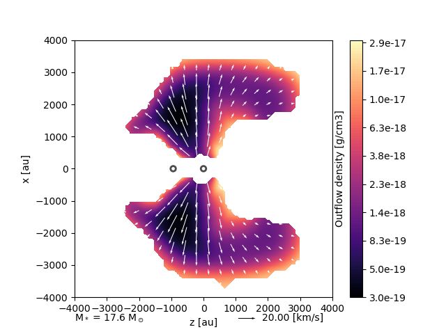
R. Mignon-Risse et al.: A new Hybrid Radiative Transfer Method for Massive Star Formation

absorption coefficient. Equation (1) must be solved at each hy-       method, the computing cost does not scale with the number of
drodynamical time-step to evolve the radiation field, which still     sources.
depends on six variables (x, n, ν). In addition, we want to cou-          Our goal is to take advantage of both methods, i.e. the FLD
ple it to hydrodynamics. This motivates the need for taking mo-       method for an optically-thick medium and M1 for irradiation.
ments of the equation of radiative transfer. Hence we loose some      Both FLD and M1 methods described above can involve several
of the angular information but it reduces the number of variables     groups of photons or only one with frequency-averaged opaci-
to four, at each time-step. The radiative energy density Eν , the     ties. In our study however we restrict ourselves to one group of
radiative flux Fν and the radiative pressure tensor Pν are defined    photons treated with each method.
as the 0-th, 1-st and 2-nd moments of the radiative intensity Iν ,        In massive star formation simulations the dynamical influ-
respectively.                                                         ence exerted by the radiative feedback is of main importance,
    Each system of moment equations involves the i-th and the         as well as the thermal structure of the accretion flow (e.g. for
(i + 1)-th moments, hence we need a closure relation. The FLD         fragmentation). However, doing so requires to:
scheme is based on the diffusion approximation, which is suited
for high optical depths, when photons propagate in a random             – retain to some extent the directionality of the photons emitted
walk in the material (e.g. in stellar interiors). It has been com-        by the star to compute the direct radiative force. Breaking
monly used as a first step to introduce radiation into hydrody-           this isotropy is consistent with probing non-isotropic modes
namical codes (Krumholz et al. 2007, Kuiper et al. 2008, Tomida           of accretion (disk or filaments);
et al. 2010). In the FLD model, the equation to be solved is the        – distinguish the opacities between stellar photons, which have
equation of conservation of the radiative energy. Once integrated         a UV-like energy and relatively high opacities, and photons
over all frequencies (often called a gray approximation) it gives         emitted by the dust, which have a IR-like energy and rela-
                                                                          tively low opacities.
∂Er
                     !
              cλ
      −∇·         ∇Er = κP ρc aT 4 − Er ,                       (2)   Our method is to inject the stellar photons into the group of pho-
 ∂t          κR ρ                                                     tons treated with the M1 scheme. The gray opacity used with the
where Er is the frequency-integrated radiative energy, λ is the       M1 corresponds to the Planck mean opacity at the stellar tem-
flux-limiter and is built to recover the right propagation speed      perature, κP (T ? ), written κP,? for the sake of readability. Once
in optically-thin and -thick media (Levermore & Pomraning             these photons are absorbed by the medium, they are depleted
1981). κP and κR are Planck’s and Rosseland’s mean opacities,         from the M1 group as they heat the gas. The gas re-emission is
respectively. Thermal radiation is modeled as the Planck func-        treated with the FLD method. In a first approach, we do not deal
tion B(ν, T ), therefore under the gray model Planck’s and Rosse-     with ionization states and leave this to further work. The set of
land’s opacities are respectively defined as                          equations that are to be solved are

                                                                              ∂EM1
      R∞
          κν B(ν)dν                                                                 + ∇ · FM1 = −κP,? ρcEM1 + ĖM1   ?
                                                                                                                        ,
κP = 0R ∞            ,                                        (3)               ∂t
        0
           B(ν)dν                                                            ∂FM1
                                                                                   + c2 ∇ · PM1 = −κP,? ρcFM1 ,
and                                                                           ∂t
                                                                       ∂Efld
                                                                                               !
       R ∞ ∂B(ν, T )                                                                cλ
                                                                             −∇·          ∇Efld = κP,fld ρc aT 4 − Efld ,
                     dν                                                 ∂t         κR,fld
κR = R
        0    ∂T          .
        ∞ 1 ∂B(ν, T )
                                                                (4)                          ∂T
                      dν                                                                  Cv     = κP,? ρcEM1 + κP,fld ρc Efld − aT 4 ,
       0 κν   ∂T                                                                             ∂t
                                                                                                                                       (6)
where the temperature derivatives appear from the chain rule ap-
                                                                               ?
plied to ∇B. The aT 4 term in Eq. 2 arises from the integral of the   where ĖM1   is the stellar radiation injection term, and κP,? ρcEM1
Planck function over all frequencies, with a the radiation con-       couples the M1 and the FLD methods via the equation of evolu-
stant. We approximate the mean opacity of the radiative energy        tion of the internal energy. We use the ideal gas relation for the
term as the Planck mean opacity.                                      internal specific energy  = Cv T where Cv is the specific heat ca-
    On the other hand, with the M1 method we take the zeroth          pacity at constant volume. This equation closes the system and
and first moments of the equation of radiative transfer (Lever-       is used to evolve the gas temperature together with the radiative
more 1984). Within the M1 method we obtain the following sys-         quantities.
tem for the radiative energy and flux conservation, in the gray
approximation as well                                                 2.2. Radiative acceleration
∂Er
    + ∇ · Fr = −ρκP cEr + Ėr? ,                                      In addition of improving the thermal coupling between stellar
 ∂t                                                             (5)   irradiation and gas, our implementation is meant to affect the gas
∂Fr                                                                   dynamics via a more accurate and less isotropic approach for
    + c2 ∇ · Pr = −ρκP cFr ,
 ∂t                                                                   the radiative acceleration than the FLD approximation, thanks
                                                                      to the equation of evolution of the stellar radiative flux. We are
where Ėr? is the rate of radiative energy injected from stellar      interested in comparing the radiative acceleration with the hybrid
sources. Fr and Pr are the frequency-integrated radiative flux and    method and with the pure FLD method.
pressure respectively.                                                    In the frame of RHD (for the full expression of RHD equa-
    One main asset is that the directionality of the photons beam     tions we refer the reader to Mihalas 1984), the radiative acceler-
is well-retained. The M1 method is able to model shadows to           ation at a given frequency is equal to
some extent (see González et al. 2007), in an irradiated accretion
disk for instance, while FLD is not. In addition, as a moment          arad,ν = κν Fν /c.                                             (7)
                                                                                                              Article number, page 3 of 17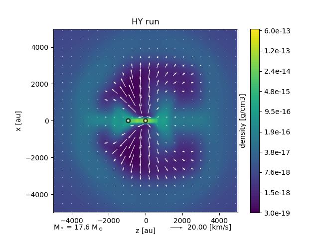
A&A proofs: manuscript no. output

    However, gray FLD and M1 methods do not share the same                 Table 1. Results from pure radiative transfer tests.
expression for the radiative flux. On one hand, the M1 model                       Ref.                     τ     T ? (K)   Method   (∆T )max,r (%)
includes the Planck mean opacity as the flux-averaged opacity —                    Pascucci et al. (2004)   0.1     5800    FLD          62
which means that momentum is transferred each time a photon                                                                 Hybrid        2
                                                                                                            0.1   15 000    FLD          65
is absorbed — so the radiative acceleration is given by                                                                     Hybrid        3
                                                                                   Pascucci et al. (2004)   100    5800     FLD          36
arad,M1 = κP,? FM1 /c.                                              (8)                                                     Hybrid       25
                                                                                                            100   15 000    FLD          57
                                                                                                                            Hybrid       31
   On the other hand, the gray radiative acceleration in the FLD                   Pinte et al. (2009)      103    4000     FLD          94
approximation is given by                                                                                                   Hybrid       76

            λ
arad,fld = − ∇Efld .                                                (9)         On one hand, the FLD solver for diffusion and radiation-
            ρ
                                                                           matter coupling is implicit and therefore is unconditionally sta-
    Taking into account the asymptotic values of λ (see Lever-             ble. The system composed of the internal energy and the radia-
more 1984), we get arad,thin = κR Efld in the limits of low optical        tive energy equations in their discretized form leads to the inver-
                                                                           sion of a matrix computed with the conjugate gradient or bicon-
depth and arad,thick = 3ρ
                        1
                          ∇Efld for high optical depth.
                                                                           jugate gradient algorithm, in case of multigroup radiative trans-
    We recall that κR is a harmonic mean which favors low ab-              fer (González et al. 2015). The number of iterations to converge
sorption bands, while κP is an arithmetic mean which favors                scales with the number of cells. Note that the isotropic radiative
high absorption bands. As a consequence, we expect a higher                pressure contributes to the total pressure in the explicit solver of
radiative acceleration with the hybrid method than with the FLD            Ramses, which therefore must satisfy the CFL condition. Hence,
method.                                                                    the radiative pressure must be taken into account when com-
                                                                           puting the timestep allowed by the CFL condition (Commerçon
2.3. Implementation                                                        et al. 2011a).
                                                                                On the other hand, the M1 solver is fully explicit with a
The Ramses code (Teyssier 2002) is a 3D adaptive-mesh refine-              first-order Godunov scheme, thus it obeys the CFL condition.
ment Eulerian code. We use a version of Ramses which has been              The trick used here is the reduced speed-of-light approximation
widely used for star formation simulations (Commerçon et al.               (Gnedin & Abel 2001). In this approximation, the propagation
2011a, 2012 , Joos et al. 2012, Hennebelle et al. 2016, Vaytet             of light is not restricted by the speed of light but by the speed
et al. 2018).                                                              of the fastest wave, which is the speed of ionization front in the
    The hydrodynamical solver of Ramses relies on finite vol-              original paper and the fastest hydro speed in our case. An addi-
ume methods (variables are volume-averaged over the cell), and             tional subcycling method relaxes this constraint. This leads to a
a second-order Godunov method is used to evolve hydro vari-                time-step set by the hydrodynamical CFL condition.
ables. This code includes the FLD (Commerçon et al. 2011b,                      The injection of energy from the stellar source into the M1
C11 hereafter) and the M1 method within Ramses-RT (Rosdahl                 photons is made via a sink algorithm (Bleuler & Teyssier 2014).
et al. 20131 , R13 hereafter), both coupled to the hydrodynamics.          In this work, we retrict ourselves to one stellar source for the M1
For the FLD method, a time-splitting approach is performed. A              photons. The M1 module ensures the propagation and absorp-
predictor-corrector MUSCL scheme is used, where the predictor              tion of the stellar radiation while the FLD module deals with
step is made under the diffusion approximation, i.e. the radiative         the heating by the stellar radiation and treats the reemission. We
pressure is isotropic, and non-isotropy is taken into account in           test the accuracy of the hybrid approach compared to the FLD
the corrector step. The hyperbolic part of the FLD solver relies           module alone, as it was used in previous massive star formation
on the second-order Godunov scheme of Ramses, and fluxes are               calculations with the Ramses code (Commerçon et al. 2011a).
estimated with an approximate Riemann solver (Lax-Friedrich,
HLL, HLLD, etc.). The diffusion and radiation-matter coupling
are handled in the implicit part of the time-splitting scheme.             3. Numerical tests
The diffusion part of the FLD solver is second-order accurate in
space. The M1 module estimates fluxes with a Riemann solver                We test the hybrid method in a pure radiative transfer case (i.e.,
(HLL or GLF). In this work we use the GLF solver, as it captures           no hydrodynamics): a static disk irradiated by a star. We com-
better the isotropy of stellar radiation that HLL, and the reduced         pare the temperature structure obtained with results from Monte-
flux approximation for the direct radiative force (see Appendix            Carlo radiative transfer codes. We explore three levels of optical
B of Rosdahl et al. 2015 and discussion in Hopkins & Grudić               thickness integrated along the disk mid-plane: τ = 0.1, τ = 100
2019).                                                                     and τ = 103 . The parameters and results are summarized in Ta-
    The radiative transfer puts a heavy constraint on the time-            ble 1. We refer the reader to Appendix B for performance tests.
step because the Courant-Friedrich-Lewy (CFL) condition for-
bids the propagation of signals through more than one cell in              3.1. Optically-thin and moderately optically-thick regimes:
one time-step, for explicit schemes. For the hydrodynamics this                 Pascucci’s test
speed is the sound speed but for radiative transfer this is the
speed of light, and this would impose a time-step ∼1000 times              3.1.1. Physical and numerical configurations
shorter. Therefore, both C11 with the FLD method and R13 with
                                                                           The first test we have performed is taken from Pascucci et al.
the M1 scheme have used a workaround.
                                                                           (2004), and consists of a star irradiating a static disk made of
1
   They express quantities in terms of photon number densities and con-    dust and gas. We use it to probe the behavior and accuracy of
sider several photo-absorbing species (H i, He i and He ii) while we fo-   our method in the optically-thin and moderately optically-thick
cus on a dust-and-gas mixture.                                             regimes. In particular, we compare our results, once the temper-
Article number, page 4 of 17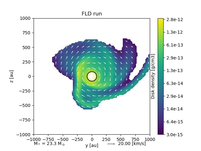
R. Mignon-Risse et al.: A new Hybrid Radiative Transfer Method for Massive Star Formation
wavelength [ m] two functions given by
3000 300 30 3 0.3
103 10 1 !−1
abs B (Tdisk) f1 (r) =
r
, (11)
sca B (T ) 10 2
rd
102 ext
10 3
and
101 10 4
B (T) [erg/cm2]
π z 2
!
[cm2g 1]
10 5 f2 (r, z) = exp − , (12)
100 4 h(r)
10 6
10 1 where the flaring function is
10 7
!1.125
10 2
10 8
h(r) = zd
r
. (13)
rd
10 9
10 3
1011 1012 1013 1014 1015 rd = rout /2 = 500 AU and zd = rout /8 = 125 AU are the
[Hz] scale-radius and the scale-height. The star is not resolved, but
its luminosity is based on its physical radius and temperature. In
Fig. 1. Frequency-dependent opacities and blackbody spectra for T disk = this test, it has a radius R? = 1 R and can have two possible
300 K and T ? = 5800 K. Opacities are absorption (blue pluses), scat- surface temperature: T ?,1 = 5800 K and T ?,2 = 15000 K.
tering (red crosses) and extinction (black dots) coefficients for the dust- The integrated optical depth (for extinction, as in the liter-
and-gas mixture used in the Pasccuci test. The table contains 61 fre- ature) is taken to be either τ = 0.1 or τ = 100 at 550 nm, to
quency bins and data are taken from Draine & Lee (1984). Apart from
probe the optically-thin and moderately optically-thick regimes,
the broad opacity features at about 10 and 20 µm, which correspond
to Si-O vibrational transitions, the opacity generally increases with the respectively. The dust-to-gas mass ratio is equal to 0.01. Dust is
photon frequency. The opacity at stellar-like radiation frequencies is made of spherical astronomical silicates of radius 0.12 micron
generally greater than at disk-like radiation frequencies. and density of 3.6 g cm−3 . Frequency-dependent dust opacities
are taken from Draine & Lee (1984) as in Pascucci et al. (2004)
and are displayed in Fig. 1. In these setups we take into account
the absorption only and neglect scattering. The corresponding
Planck and Rosseland mean opacities used in the gray M1 and
102 P [cm2 g 1] FLD modules are displayed in Fig. 2. We recall that we take the
R [cm2 g 1]
M1 absorption coefficient as the Planck mean opacity at the stel-
101 lar temperature, κP (T ? ).
mean opacity [cm2 g 1]
Boundary conditions are chosen to be a fixed temperature
of 14.8K and a density floor of 10−23 g cm−3 . The same density
100 floor is applied between the star and the disk edge, in order to
mimic the vacuum that RADMC-3D and MCFOST strictly ap-
10 1 ply as their cylindrical/spherical grids begin at Rin . The 14.8K
temperature is applied throughout the computational domain as
initial condition and is at equilibrium with the radiation.
10 2 We run the simulations with AMR levels between 5 and 14,
which results in a finest resolution of ∆x = 0.12 AU, where ∆x is
the cell width. This allows to have several (≈9) cells between the
101 102 103 104 star and the disk edge, and the star to have a negligible size com-
T [K] pared to the disk thickness (≈0.01 AU against ≈0.04 AU for the
Fig. 2. Planck’s (blue dashed curve) and Rosseland’s (orange dot- disk height at rin ). Secondly, it permits to resolve several times
dashed curve) mean opacities, as a function of temperature in the Pas- the mean free-path at the disk inner edge: the local optical depth
cucci setup. is κP ρmax ∆x≈0.15 < 1, where ρmax is the density at the disk
inner edge, for the case τ = 100. Refinement is performed on
the density gradient so that the disk inner edge is at the highest
ature structure is converged with respect to time, with those ob- refinement level. We consider that the temperature structure is
tained with Monte-Carlo RT codes such as RADMC-3D (Dulle- converged when the relative change between successive outputs
mond et al. 2012) and MCFOST (Pinte et al. 2006). decreases below 10−4 (see Ramsey & Dullemond 2015).
This is a 2D test of a static flared disk of a given analytical
profile for the gas density, depending on the cylindrical radius r
3.1.2. Temperature structure
and on the vertical height z. The disk extends from rin = 1 AU to
rout = 1000 AU. The density ρ(r, z) in cylindrical coordinates is The Ramses grid is Cartesian while the grids of MCFOST and
given as RADMC-3D are cylindrical and spherical, respectively. There-
fore, we interpolate temperature values on their grids to compute
ρ(r, z) = ρ0 f1 (r) f2 (r, z), (10) the relative error at the location on the Ramses grid. Figure 3
plots the gas temperature in the disk mid-plane with respect to
where ρ0 is the density normalization and is linked to the the x-axis, for the most optically-thin case, τ = 0.1, once the
only free-parameter, the integrated
R rout optical-depth throughout the temperature structure is converged with respect to time. The lo-
mid-plane of the disk, τν = r κν ρ(r, z = 0) dr. f1 and f2 are cation is given by the distance to the disk inner edge, r − rin . For
in
Article number, page 5 of 17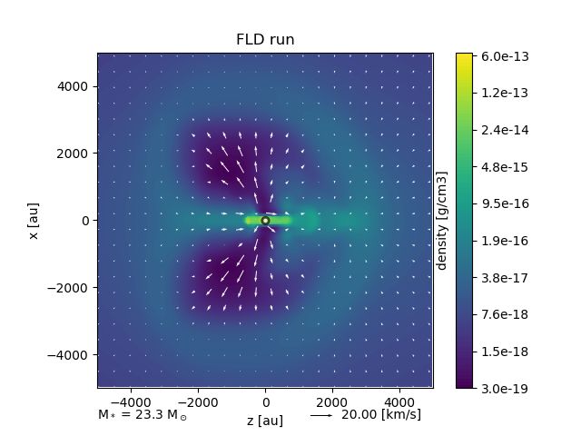
A&A proofs: manuscript no. output

                                         T = 5800 K, = 0.1                                                                 T = 15000 K, = 0.1
                                                                   Hybrid                                                                             Hybrid
                                                                   FLD                                      103                                       FLD
   Gas temperature [K]

                                                                                      Gas temperature [K]
                                                                   RADMC-3D                                                                           RADMC-3D
                         102                                       MCFOST

                                                                                                            102

                               10   1   100        101       102           103                              50    10   1   100        101       102          103

                                                                                    Relative error [%]
                           0
 relative error [%]

                         25                                                                                   0
                         50                                                                                 50
                               10   1   100        101       102           103                                    10   1   100         101      102          103
                                              R Rin [AU]                                                                         R Rin [AU]
Fig. 3. Radial gas temperature profiles in the mid-plane of the disk following the test of Pascucci et al. (2004) for τ = 0.1. We compare the gas
temperature computed using MCFOST (black dotted-line) and/or RADMC-3D (red dashed-line), the hybrid method (M1+FLD, blue dots) and the
FLD method alone (orange dots) in Ramses. Left: central star temperature T ?,1 = 5800K; right: T ?,2 = 15000K.

T ?,1 and T ?,2 the FLD run produces an important error through-                       the hybrid method. Indeed, the temperature varies significantly
out the disk mid-plane, up to ≈62% and ≈65%, respectively,                             throughout the disk (between ≈20 and 350 K for T ?,1 and be-
and always underestimates the temperature. On the opposite, the                        tween ≈20 and 1000 K for T ?,2 ). As a consequence, a disk cell
hybrid method is quite accurate with a maximal error of ≈3%,                           is crossed by photons of very different frequencies, and the gray
while RT codes (MCFOST and RADMC-3D) agree within 1%                                   approach induces errors. Conversely, the frequency-dependence
in this test (in accord with Pascucci et al. 2004). This impor-                        of RADMC-3D method permits to distinguish the photons that
tant difference between FLD and hybrid methods comes from the                          are quickly absorbed (the most energetic ones) from those, at
regime of validity of each method: the FLD is not well-suited for                      lower energy, that will penetrate the disk more deeply and con-
optically-thin media. In the hybrid method, as there is not much                       tribute to the disk heating at larger radii.
absorption because of the low optical-depth, the M1 module is                               To examine the behavior of both methods with respect to the
mainly at work and is adapted to optically-thin media (as tested                       non-isotropy of the setup we plot the vertical temperature pro-
in Rosdahl et al. 2013), which justifies its good accuracy.                            file at a cylindrical radius of 20 AU (Fig. 5). This visualization
     For direct irradiation, the Planck mean opacity in the FLD                        is important for this type of tests, as an optically-thick disk pro-
implementation is computed at the local temperature, even                              duces self-shielding in the mid-plane and we expect the hybrid
though the radiation was emitted by the star. A direct conse-                          method to capture it better than the FLD method (González et al.
quence is that the stellar radiation is absorbed by the disk with                      2007). Here we take the temperature given by MCFOST rather
an opacity coefficient computed at the disk temperature, which is                      than RADMC-3D because its grid is cylindrical (and not spheri-
much lower than the stellar temperature. As the opacity increases                      cal) and thus errors of interpolation are avoided. The left panel of
with the temperature (see Fig. 2), the absorption opacity with the                     Fig. 5 shows the temperature profile for the most optically-thin
FLD is lower and hence the temperature is lower than that given                        case, τ = 0.1. No self-shielding is expected and the temperature
by RT codes and by the hybrid approach. The situation worsens                          should decrease slowly as the vertical height increases. Such a
from T ?,1 to T ?,2 at the disk edge and the error increases from                      behavior is obtained with MCFOST as well as with the hybrid
≈30% to ≈60%. It also illustrates the need for a better approach                       method. The temperature obtained with the FLD method is uni-
for treating massive stars irradiation.                                                form with z, which is likely due to the isotropic nature of the
                                                                                       FLD method. The relative error is comparable to the one in the
     The left panel of Fig. 4 shows the radial temperature profile
                                                                                       radial profile: up to ≈47% with the FLD method and less than
in the disk mid-plane for the moderately optically-thick case,
                                                                                       1% with the hybrid approach.
τ = 100, and for T ?,1 . The error made by the hybrid method is
higher than for the τ = 0.1 case and reaches a maximal value of                             On the right panel of Fig. 5, τ = 100, and MCFOST gives a
≈25%, whereas the FLD method alone makes a maximal error of                            lower temperature in the mid-plane than for τ = 0.1, as expected.
≈36%. Also, the error made by the hybrid method is quite uni-                          Conversely, the FLD method does not capture at all the non-
form, compared to the error made by the FLD method alone.                              isotropic nature of the radiation onto the irradiated disk: the tem-
For T ?,1 and T ?,2 (left and right panels of Figs. 3 and 4, re-                       perature is fairly uniform. The hybrid method reproduces partly
spectively), the FLD method underestimates the temperature be-                         this feature, even though the error can be as large as ≈20%.
tween the star and the disk edge because the medium is optically                            We conclude that the FLD method is not capable of repro-
thin and because of the Planck opacity considered, as explained                        ducing the temperature profile in the optically-thin and moder-
above. For T ?,2 , both methods converge toward a similar tem-                         ately optically-thick regime. The hybrid method is very accurate
perature at large radii. Absorption is stronger here than in the                       in the optically-thin regime (less than ≈2%). In the moderately
most optically-thin case, and stronger than for T ?,1 (see Fig. 2),                    optically-thick regime, the hybrid method gives a non-negligible
so the M1 photons are quickly absorbed and the FLD module                              error (up to ≈31% for a 15000 K star) in the transition between
of our hybrid method is at work. Therefore a significant error is                      optically-thin and -thick media which shows its limitations, but
expected from the gray opacity employed in the FLD module of                           this is a major improvement compared to the ≈57% error made
Article number, page 6 of 17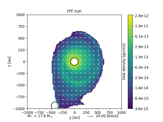
R. Mignon-Risse et al.: A new Hybrid Radiative Transfer Method for Massive Star Formation
T = 5800 K, = 100 T = 15000 K, = 100
Hybrid Hybrid
FLD 103 FLD
Gas temperature [K]
Gas temperature [K]
RADMC-3D RADMC-3D
102 MCFOST
102
25 10 1 100 101 102 103 10 1 100 101 102 103
Relative error [%]
relative error [%]
0 0
25
50
10 1 100 101 102 103 10 1 100 101 102 103
R Rin [AU] R Rin [AU]
Fig. 4. Same as Fig. 3 for τ = 100.
T = 5800 K, = 0.1 T = 5800 K, = 100
100 100
Gas temperature [K]
Gas temperature [K]
90 90
Hybrid Hybrid
80 FLD 80 FLD
MCFOST MCFOST
70 70
60 60
2.5 5.0 7.5 10.0 12.5 15.0 17.5 2.5 5.0 7.5 10.0 12.5 15.0 17.5
Relative error [%]
Relative error [%]
0
20 0
25
40
2.5 5.0 7.5 10.0 12.5 15.0 17.5 2.5 5.0 7.5 10.0 12.5 15.0 17.5
z [AU] z [AU]
Fig. 5. Vertical gas temperature profiles at a cylindrical radius of 20 AU, following the test of Pascucci et al. (2004). We compare the gas
temperature computed using MCFOST, the hybrid method (M1+FLD) and FLD alone in Ramses for T ?,1 , τ = 0.1 (left) and τ = 100 (right).
with the FLD method. In addition, the hybrid approach captures The right panel of Fig. 6 shows the sum of the FLD and M1
partially (≈20% error) the self-shielding in the disk mid-plane radiative accelerations in the hybrid case. The combination of
while the FLD approximation does not. the optically-thin and -thick methods permits to capture the non-
isotropy of the radiative acceleration. The hybrid radiative ac-
celeration is ∼100 greater than the FLD acceleration. This result
3.1.3. Impact on the radiative acceleration holds in the four tests: τ = 0.1, τ = 100 and T ?,1 , T ?,2 . This num-
ber is in agreement with the study of Owen et al. (2014). This is
mainly due to the temperature at which the M1 opacity is taken.
We look at the radiative acceleration maps obtained with the
Stellar photons are at a frequency that is ∼10 times greater than
FLD and the hybrid methods for the moderately optically-thick
that of photons emitted by the surrounding gas, which implies
case (τ = 100). Figure 6 shows the radiative acceleration perpen-
an opacity ∼100 greater (see Fig. 1). As shown previously, the
dicularly to the disk plane as obtained after temperature conver-
radiation transport in the optically-thin limit is accurately treated
gence with the FLD method (left) and the hybrid method (right).
with our hybrid approach and leads to a strong improvement for
The left panel shows two peculiarities of the FLD solver. First,
the radiative acceleration due to the direct irradiation, which is
we recall that the FLD radiative acceleration has two asymptotic
one of the main contributors expected in the dynamics of mas-
values depending on the optical regime (see subsection 2.2): in
sive star formation.
the optically-thin limit it is proportional to the radiative energy
and in the optically-thick limit it is equal to the radiative energy
gradient divided by the density. Further from the star, the disk 3.2. Optically-thick regime: Pinte’s test
structure is visible (the dark blue zones) because of the density
dependence in the radiative acceleration. Second, the aspect of The second test is a similar but more challenging setup, with
the FLD acceleration closer to the star is mainly due to grid ef- a higher integrated optical depth and a sharper density profile
fects. than Pascucci et al. (2004) at the disk edge, as presented in Pinte
Article number, page 7 of 17A&A proofs: manuscript no. output
FLD 4.127
Hybrid 4.127
400 5.059 400 5.059
5.990 5.990
200 6.922 200 6.922
log(ahy) [cm s-2]
log(afld) [cm s-2]
7.854 7.854
z [au]
z [au]
0 8.785 0 8.785
9.717 9.717
200 10.649 200 10.649
11.580 11.580
400 400
12.512 12.512
400 200 0 200 400 400 200 0 200 400
y [au] y [au]
Fig. 6. 1000 AU disk edge-on slices of the radiative acceleration, following the test of Pascucci et al. (2004) obtained with Ramses after stationarity
is reached. Left: FLD run; right: hybrid run. Star and disk parameters: τ = 100 and T ?,1 . The hybrid radiative acceleration is about 100 times greater
than the FLD one.
of photon absorption, which leads to overestimating the temper-
ature. Resolving both is even more challenging for AMR-grid
codes than for cylindrical-grid codes with no material inside Rin
and a logarithmic scale. In Ramses we choose to refine the grid
based on a density gradient criterion so that the disk edge is at
the finest resolution and the transition from optically-thin to -
thick is as resolved as possible. There is a drawback: having the
greatest resolution at the disk inner edge is very computationally
expensive because, first, it affects many more cells than if the re-
finement is operated on the central cell (as usually done because
the sink particle is located there). In addition, two adjacent cells
cannot differ by more than one level of refinement and gener-
ally the number of cells at the same AMR level is much higher
than two. Therefore, it also means a higher resolution at larger
radii. For that reason, Ramsey & Dullemond (2015) choose not
to use AMR but instead, a logarithmically-scaled grid particu-
larly adapted to this setup. Figure 7 shows the AMR level needed
to resolve the local mean free path, as a function of the radius in
Fig. 7. AMR level needed to resolve the mean free path (mfp) of pho- the disk midplane, along with the AMR level set with Ramses.
tons (red dashed-line) and effective AMR level (black dots) in the disk Hence, we perform our calculations with lmax = 22, which gives
midplane following the test of Pinte et al. (2009). a finest cell width of 1.9 × 10⁻⁴ AU, so that the mean free path
at the disk inner edge is resolved. The computational cost does
et al. (2009). The disk extends from a cylindrical radius rin = not allow to extend the zone over which the mean free path is
0.1 AU to rout = 400 AU, and the integrated optical depth (for resolved, nor to compare the temperature over the entire disk ra-
extinction) is τ810nm = 103 . The flared disk density profile ρ(r, z) dius with RADMC-3D.
is analytically given by The left panel of Fig. 8 plots the radial temperature profile in
!−2.625 the disk mid-plane obtained with Ramses with the FLD and hy-
1 z 2
!
r brid methods versus RADMC-3D. FLD underestimates the tem-
ρ(r, z) = ρ0 exp − , (14) perature at the disk inner edge, as in the test of Pascucci et al.
rd 2 h(r)
(2004). The temperature slope given by the hybrid method is in
where the flaring function h(r) is as before, rd = rout /4 = 100 AU a better agreement with RADMC-3D than the one given by the
and zd = rout /40 = 10 AU. The star has a radius R? = 2 R and FLD method. For the hybrid method, the temperature at the in-
the stellar surface temperature is T ? = 4000 K. ner edge of the disk is accurately computed (up to ≈7% error)
We use the opacity table from Weingartner & Draine (2001) but is overestimated at larger radii where it becomes fairly con-
which gives the absorption opacity of dust grains with respect stant at ≈65% error. It can be seen that the error made by the
to the wavelength. These opacities were calculated for spherical hybrid approach is not negligible as the mean free path becomes
astronomical silicates (see Draine & Lee 1984) of size 1 micron unresolved (Fig. 7). The temperature profile obtained with our
and density 3.6 g cm−3 . hybrid method is very similar to what has been obtained in sim-
The sharp increase in density at the disk inner edge makes ilar studies (see Fig. 8 of Ramsey & Dullemond 2015).
this test particularly challenging because the local variation of The right panel of Fig. 8 shows the vertical temperature pro-
optical depth must be resolved, as the discretized equations in- file. The temperature profile shape given by the hybrid method
volve locally constant absorption opacities. At the same time, it is similar to RADMC-3D but with self-shielding partially cap-
is crucial to resolve the local mean free path to prevent an excess tured (up to ≈61% error), unlike in the FLD method. The hybrid
Article number, page 8 of 17R. Mignon-Risse et al.: A new Hybrid Radiative Transfer Method for Massive Star Formation
Fig. 8. Left: radial gas temperature profiles in the mid-plane of the disk following the test of Pinte et al. (2009). Right: vertical gas temperature
profiles at a cylindrical radius of 0.2 AU in the disk. We compare the gas temperature computed using RADMC-3D, the hybrid method (M1+FLD)
and the FLD method alone in Ramses. The integrated optical depth in the disk mid-plane is τ810nm = 103 and the stellar temperature is T ? = 4000 K.
method then recovers the correct temperature (≈2% error) at a Mdust
where Mgas is the initial dust-to-gas mass ratio, and the evap-
larger disk height. 0
This setup highlights the need to resolve the mean free path oration temperature is given by
of photons to obtain the correct temperature at the disk edge, T evap (ρ) = gρβ (16)
and it shows that the hybrid approach is more accurate than the
FLD approximation to compute the temperature structure of an with g = 2000 K cm3 g−1 , β = 0.0195 (Isella & Natta 2005).
optically-thick disk. Moreover, this setup is challenging for our At high temperature, when all dust grains are evaporated, the
hybrid method because most of the direct irradiation is absorbed gas opacity is dominant and is taken equal to 0.01 cm2 g−1 for
in the inner parts of the disk so the rest of the disk temperature comparison purposes with previous studies, such as Krumholz
structure is mainly obtained with the FLD method. As shown in et al. 2009, Kuiper et al. 2014, Rosen et al. 2016, Klassen et al.
Ramsey & Dullemond (2015), a frequency-dependent irradiation 2016.
scheme is not more accurate in this test. However, a multigroup
FLD method (González et al. 2015) would improve this, as men-
tioned by Ramsey & Dullemond (2015). 4.2. Setup
We start from initial conditions similar to Rosen et al. (2016): a
4. Collapse of an isolated massive prestellar core 150 M spherical cloud of radius 0.1 pc in a box of size 0.4 pc
to limit boundary effects. The density profile is spherically-
We use the newly implemented and tested hybrid method in the symmetric and ρ(r) ∝ r−1.5 . The free-fall time is then
context of a massive star formation and study the influence of
using such a radiation transport method with respect to the pre- s
3π
viously used Flux-Limited Diffusion approximation. τff = ' 42.5 kyr, (17)
32Gρ̄
4.1. Included physics where G is the gravitational constant, and ρ̄ is the mean den-
Our simulations are run with the Ramses code (Teyssier 2002) sity computed for a uniform sphere. The density at the border
which includes a hydrodynamics solver, sink particle algorithm of the cloud is 100 times the density of the ambient medium.
(Bleuler & Teyssier 2014), and radiative transfer with either the The cloud is in solid-body rotation around the x-axis with rota-
Flux-Limited Diffusion module alone (which we call the FLD tional to gravitational energy of ≈4%, typical of observed cores
run) or coupled to Ramses-RT (the HY run) within our hybrid (Goodman
et al. 1993). The initial dust-to-gas mass ratio is
approach. The opacities were originally used in the low-mass Mdust
Mgas = 0.01.
star formation calculations of Vaytet et al. (2013) which include 0
The base resolution is level 7 (1283 ) and the finest resolution
frequency-dependent dust opacities (T < 1500 K, Semenov et al.
is 40963 (i.e. level 12, five levels of refinement), which gives a
2003, Draine 2003). We modify the gray opacities to account for
physical maximum resolution of 20 AU. In order to limit arti-
dust sublimation, as its importance for the shielding properties
ficial fragmentation (Truelove et al. 1997), we impose to have
of massive disks has been highlighted in Kuiper et al. (2010b).
at least 12 cells per Jeans length. Sink particles can only form in
We model it in the same way as Kuiper et al. (2010a) (Eqs (21)
cells refined to the highest level. Sink creation sites are identified
and (22) therein) with a dust-to-gas ratio that decreases with tem-
with the clump finder algorithm of Bleuler & Teyssier (2014).
perature, and a sublimation temperature that increases with the
The clump finder algorithm marks cells whose density is above
density. The profile of the dust-to-gas mass ratio is given by
! !! a given threshold (3.85 × 10⁻¹⁴ g cm−3 in these calculations. The
Mdust Mdust 1 T − T evap (ρ) marked cells are attached to their closest density peak, which
(ρ, T ) = 0.5 − arctan (15)
Mgas Mgas 0 π 100 form a "peak patch". We check connectivity between the patches,
Article number, page 9 of 17A&A proofs: manuscript no. output
then the significance of a peak patch is given by the ratio be- As it is shown on the top-right panel of Fig. 9, the stars ex-
tween the peak density and the maximum saddle density lying at perience bursts of accretion separated by ∼100 yrs to a few kyr.
a boundary of the peak patch. If the peak-to-saddle ratio is lower These bursts are due to a low-mass companion (sink particle) be-
than a given value (2 here), the patch is attached to the neighbor ing accreted by the most massive star. In each run, the main sink
patch of highest saddle density. The remaining peak patches are experiences accretion rates of M ∼10−4 −10−2 M .yr−1 , which is
labeled as clumps. Each clump must then meet two conditions consistent with previous numerical studies (Klassen et al. 2016)
to lead to a sink creation: it has to be bound and subvirial. The and observations (review by Motte et al. 2018 and references
region around a sink particle is also refined to the highest level. therein).
The accretion scheme is based on a density threshold. Consider
a cell located within the accretion radius: its accreted mass by
4.3.1. Disk properties
the sink is ∆m = max(0.25(ρ − ρsink )(∆x3 , 0), where ∆x is the
maximum resolution. We merge sinks when they are located in As shown in the bottom-left panel of Fig. 9, the disks obtained
the same accretion volume, while the accretion radius is set to are massive (≈17 M at the end of the simulation) and similar
4∆x ≈ 80 AU. This rough operation can lead to higher mass in mass in both runs. Observational constraints on the disk mass
stars and decrease the system multiplicity. The radius and lumi- remain sparse (Motte et al. 2018), but the disk mass we obtain
nosity of the star mimicked by the sink are computed from the is consistent with the previous numerical work of Klassen et al.
pre-main sequence evolution models of Kuiper & Yorke (2013), (2016).
and depend on their time-averaged accretion rate and their mass. We investigate the disk stability by computing the Toomre
parameter Q defined by
4.3. Results cs κ
Q= (18)
πGΣ
We run one simulation with FLD only (denoted as FLD) and one
with FLD+M1 (denoted as HY) until t ' 30 kyr ' 0.71τff . As where c s is the sound speed, κ is the epicyclic frequency and
the initial density profile is peaked, a sink particle is expected to is equal to the rotation frequency for a Keplerian disk and Σ is
form in a few kyr. Both runs lead to the formation of several sink the column density. We recall that the Toomre parameter com-
particles one of which is much more massive than the other sink putes the ratio of the thermal support and differential rotation
particles, and that we will refer to as the main sink or star. A disk support over gravitational fragmentation, and that the disk is lo-
and radiative outflows form around the main sink. The criteria cally unstable if Q < 1. The gas in our simulation is initially in
for determining the disk and outflows are explained below. We solid-body rotation but the disks formed indeed exhibit rotation
identify a disk on a cell-basis after converting Cartesian coordi- curves consistent with Keplerian rotation, as shown in Fig. 10.
nates into cylindrical coordinates centered on the main sink and Hence the epicyclic frequency κ is equal to Ω, the Keplerian ro-
aligned with the rotational axis, according to the several criteria tational frequency.
of Joos et al. (2012): To calculate Q, we have taken the column density integrated
over the x-axis (perpendicular to the disk). Moreover, the selec-
– The disk is a rotationally-supported structure (i.e. not ther- tion given by the criteria presented above gives a disk with a ver-
mally supported): ρv2φ /2 > fthres P, where vφ is the azimuthal tical structure. Therefore, we evaluate the Toomre Q parameter
velocity and P is the thermal pressure, and the value of in the disk selection, then we average Q over the disk height. For
fthres = 2 is chosen, as in Joos et al. (2012). The use of completeness, we have also computed Q with cs and κ evaluated
fthres > 1 leads to a stronger constraint on the identification in the disk midplane and have obtained very similar results.
of cells belonging to the disk; We also take into account the radiation as an extra-support
– In order to avoid large low-density spiral arms, a gas number against fragmentation, as the radiative pressure contributes to the
density threshold is set: n > 1 × 109 cm−3 ; sound speed (Mihalas 1984, eq. (101.22) therein)
– The gas is not on the verge of collapsing radially. vφ > P + Pr
fthres vr , where vr is the radial velocity; c2s = Γ1 (19)
ρ
– The vertical structure is in hydrostatic equilibrium: vφ >
fthres vz , where vz is the vertical velocity. where P is the gas pressure, Pr is the radiative pressure; Γ1 = 5/3
for a non-radiating fluid (Pr = 0, pure hydro case), and Γ1 '
We define outflows as gas flowing away from the central star 1.43 if Pg = Pr ). Therefore, we argue that even for a disk in a
√ a velocity greater than the escape velocity, i.e. vr > vesc =
at strong radiation field and gas-radiation coupling (Pr ∼Pg ), Q only
2GM? /r, where r is the distance between the sink and the cell, increases by a factor of ' 1.3 as compared to the pure hydro case.
and M? is the sink mass. Figure 11 displays the local Toomre Q value taking into account
The time evolution of the main sink, disk and outflow the radiative support, but the values of Q without the radiative
masses, along with the accretion rate, are displayed in Fig. 9. support lead to the same conclusions.
First, the sink masses are almost equal in both runs before As shown in Fig. 11, the disks obtained in both runs are
t ' 14 kyr and M? = 5 M . Even though their evolution dif- Toomre unstable close to the massive star and in the spiral arms.
fers between 14 kyr and 20 kyr, their values remain similar and This is consistent with the regular creation of sink particles in
the divergence appears only at t ' 20 kyr, when M? = 12 M those spiral arms. Seven low-mass short-lived companions are
(in the HY run). At that point, the radiative cavities appear in the generated in the FLD run and six in the HY run. Even though the
HY run (see the bottom-right panel of Fig. 9). They appear in appearance of sink particles is quite resolution-dependent, we
the FLD run after the massive star has reached 16 M . From this limit it with our refinement criterion based on the Jeans length.
time on, the sink mass increases more slowly in the HY run, this The left panel of Fig. 12 shows the main star mass against
can be seen on the accretion rate (top-right panel of Fig. 9). The the disk mass. Both generally increase with time, but the disk
final stellar mass is M? = 23.3 M in the FLD run and 17.6 M also undergoes losses of mass, as it feeds the main sink parti-
in the HY run. cle. Indeed, the main accretion mode in our simulation is disk
Article number, page 10 of 17R. Mignon-Risse et al.: A new Hybrid Radiative Transfer Method for Massive Star Formation
Fig. 9. Time evolution of the main sink mass (top-left panel), accretion rate (top-right), disk mass (bottom-left), and outflow mass (bottom-right).
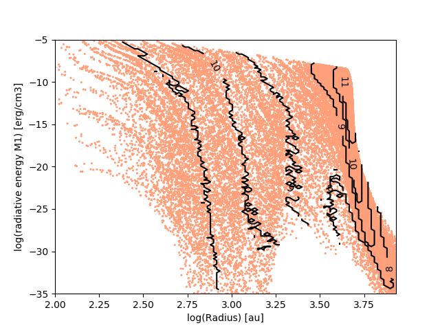
4.3.2. Radiative cavities - outflows
As mentioned in Sec. 4.3: we define outflows as gas flowing
away from the central star at a velocity greater than the escape
velocity. In the FLD run, radiative cavities appear at t ' 22
kyr (bottom-right panel of Fig. 9). They develop earlier and at
lower stellar mass (M? = 12 M , t ' 20 kyr) in the HY run
than in the FLD run (M? = 16 M , right panel of Fig. 12).
In both runs, the cavities grow symmetrically with respect to
the disk plane, until they reach an extent of ' 2000 AU in the
FLD run and ' 3000 AU in the HY run at t ' 30 kyr (see
Fig. 13). The right panels of Fig. 13 display a slice of the den-
sity within the outflow selection of cells. The gas velocity is also
higher in the HY run, ≈25 km/s, against ≈15 km/s in the FLD
run. As displayed in Fig. 14, gas is pushed away by the radia-
tive force, which locally exceeds gravity. It illustrates the flash-
light effect: the radiative force dominates in the poles while the
gravity, and hence the accretion, dominates in the disk plane.
Fig. 10. Radial rotational velocity profile in the disk cells for the HY run The consequence of the stronger radiative force is that the out-
at t = 30 kyr and Keplerian profile computed with the main stellar mass. flows in the HY run are able to transport higher density gas than
The slope of the velocity profile is consistent with Keplerian rotation. in the FLD run (see right panels of Fig. 13), mainly because it
spans a wider angle, particularly in the vicinity of the star (see
Fig. 14). Indeed, the outflows displayed in Fig. 13 have masses
Mo,HY ' 0.6 M > Mo,FLD ' 0.06 M , as displayed on the
accretion, although the accretion bursts are due to the accretion bottom-right panel of Fig. 9. During almost all the simulations
of sink particles recently created in the Toomre unstable spiral the outflows in the HY run are more massive than in the FLD
arms of the disk. The accretion in our simulation is more stable run. In addition, the temporal evolution at t ' 30 kyr seems to
than what is obtained in the work of Klassen et al. (2016), where show that this mass is still going to increase in the HY run but
the global disk instability leads to an increase of ' 10 M in a not in the FLD run. We finally note that the peak in the outflow
few kyr in their 100 M run. mass at t ' 20 kyr is due to the launching of the outflows in a
Article number, page 11 of 17You can also read