A Query-Driven System for Discovering Interesting Subgraphs in Social Media
←
→
Page content transcription
If your browser does not render page correctly, please read the page content below
Social Network Analysis and Mining manuscript No.
                                         (will be inserted by the editor)

                                         A Query-Driven System for Discovering Interesting Subgraphs
                                         in Social Media
                                         Subhasis Dasgupta ·
                                         Amarnath Gupta
arXiv:2102.09120v1 [cs.SI] 18 Feb 2021

                                         Received: date / Accepted: date

                                         Abstract Social media data are often modeled as heterogeneous graphs with multiple types of nodes and edges.
                                         We present a discovery algorithm that first chooses a “background” graph based on a user’s analytical interest
                                         and then automatically discovers subgraphs that are structurally and content-wise distinctly different from the
                                         background graph. The technique combines the notion of a group-by operation on a graph and the notion of
                                         subjective interestingness, resulting in an automated discovery of interesting subgraphs. Our experiments on a
                                         socio-political database show the effectiveness of our technique.
                                         Keywords social network · interesting subgraph discovery · subjective interestingness

                                         1 Introduction                                                tities, topics, sentiment scores) may also be used for
                                                                                                       analysis. To be practically useful, the system must
                                         An information system designed for analysis of social         accommodate semantic synonyms – #KamalaHarris,
                                         media must consider a common set properties that char-        @KamalaHarris and “Kamala Harris” refer to the
                                         acterize all social media data.                               same entity.
                                         – Information elements in social media are essentially      – Relationships between information items in social me-
                                           heterogeneous in nature – users, posts, images, exter-      dia data must capture both canonical relationships
                                           nal URL references, although related, all bear differ-      like (tweet-15 mentions user-392) but a wide-variety
                                           ent kinds information.                                      of computed relationships over base entities (users,
                                         – Most social information is temporal – a timestamp           posts, . . .) and text-derived information (e.g., named
                                           is associated with user events like the creation or re-     entities).
                                           sponse on a post, as well as system events like user
                                                                                                     It is also imperative that such an information must sup-
                                           account creation, deactivation and deletion. The sys-
                                                                                                     port three styles of analysis tasks
                                           tem should therefore allow both temporal as well as
                                           time-agnostic analyses.                                   1. Search, where the user specifies content predicate
                                         – Information in social media evolves fast. In one study       without specifying the structure of the data. For
                                           (Zhu et al., 2013), it was shown that the number             example, seeking the number of tweets related to
                                           of users in a social media is a power function of            Kamala Harris should count tweets where she is the
                                           time. More recently, (Antonakaki et al., 2018) showed        author, as well as tweets where any synonym of “Ka-
                                           that Twitter’s growth is supralinear and follows Le-         mala Haris” is in the tweet text.
                                           scovec’s model of graph evolution (Leskovec et al.,       2. Query, where the user specifies query conditions
                                           2007). Therefore, an analyst may first have to per-          based on the structure of the data. For example,
                                           form exploration tasks on the data before figuring out       tweets with create date between 9 and 9:30 am on
                                           their analysis plan.                                         January 6th, 2021, with text containing the string
                                         – Social media has a significant textual content, some-        “Pence” and that were favorited at least 100 times
                                           times with specific entity markers (e.g., mentions)          during the same time period.
                                           and topic markers (e.g., hashtags). Therefore any in-     3. Discovery, where the user may or may not know
                                           formation element derived from text (e.g., named en-         the exact predicates on the data items to be re-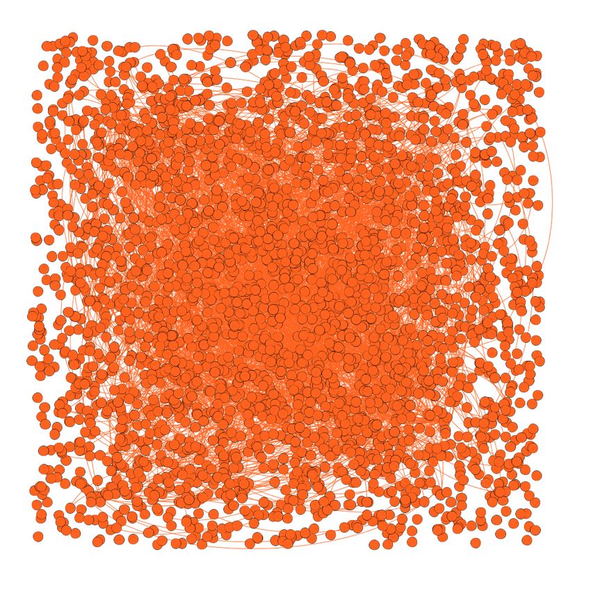
2

    trieved, but can specify analytical operations (to-     2 Related Work
    gether with some post-filters) whose results will pro-
    vide insights into the data. For example, we call a     The problem of finding “interesting” information in a
    query like Perform community detection on all           data set is not new. (Silberschatz and Tuzhilin, 1996)
    tweets on January 6, 2021 and return the usersdescribed that an“interestingness measure” can be “ob-
    from the largest community a discovery query.           jective” or “subjective”. A measure is “objective” when
                                                            it is computed solely based on the properties of the
                                                            data. In contrast, a “subjective” measure must take into
In general, a real-life analytics workload will freely com-
                                                            account the user’s perspective. They propose that (a) a
bine these modalities as part of a user’s information
                                                            pattern is interesting if it is ”surprising” to the user (un-
exploration process.
                                                            expectedness) and (b) a pattern is interesting if the user
    In this paper, we present a general-purpose graph-      can act on it to his advantage (actionability). Of these
based model for social media data and a subgraph dis-       criteria, actionability is hard to determine algorithmi-
covery algorithm atop this data model. Physically, the      cally; unexpectedness, on the other hand, can be viewed
data model is implemented on AWESOME (Dasgupta              as the departure from the user’s beliefs. For example,
et al., 2016), an analytical platform designed to enable    a user may believe that the 24-hour occurrence pattern
large-scale social media analytics over continuously ac-    of all hashtags are nearly identical. In this case, a dis-
quired data from social media APIs. The platform, de-       covery would be to find a set of hashtags and sample
veloped as a polystore system natively supports rela-       dates for which this belief is violated. Following (Geng
tional, graph and document data, and hence enables a        and Hamilton, 2006), there are three possibilities re-
user to perform complex analysis that include arbitrary     garding how a system is informed of a user’s knowledge
combinations of search, query and discovery operations.     and beliefs: (a) the user provides a formal specification
We use the term query-driven discovery to reflect           of his or her knowledge, and after obtaining the mining
that the scenario where the user does not want to run       results, the system chooses which unexpected patterns
the discovery algorithm on a large and continuously col-    to present to the user (Bing Liu et al., 1999); (b) ac-
lected body of data; rather, the user knows a starting      cording to the user’s interactive feedback, the system re-
point that can be specified as an expressive query (illus-  moves uninteresting patterns (Sahar, 1999); and (c) the
trated later), and puts bounds on the discovery process     system applies the user’s specifications as constraints
so that it terminates within an acceptable time limit.      during the mining process to narrow down the search
                                                            space and provide fewer results. Our work roughly cor-
                                                            responds to the third strategy. Early research on finding
Contributions. This paper makes the following contri-
                                                            interesting subgraphs focused primarily on finding in-
butions. (a) It offers a new formulation for the subgraph
                                                            teresting substructures. This body of research primarily
interestingness problem for social media; (b) based on
                                                            found interestingness in two directions: (a) finding fre-
this formulation, it presents a discovery algorithm for
                                                            quently occurring subgraphs in a collection of graphs
social media; (c) it demonstrates the efficacy of the al-
                                                            (e.g., chemical structures) (Kuramochi and Karypis,
gorithm on multiple data sets.
                                                            2001; Yan and Han, 2003; Thoma et al., 2010) and (b)
                                                            finding regions of a large graph that have high edge den-
Organization of the paper. The rest of the paper            sity (Lee et al., 2010; Sariyuce et al., 2015; Epasto et al.,
is organized as follows. Section 2 describes the related    2015; Wen et al., 2017) compared to other regions in the
research on interesting subgraph finding in as inves-       graph. Note that while a dense region in the graph can
tigated by researchers in Knowledge Discovery, Infor-       definitely interesting, shows, the inverse situation where
mation Management, as well Social Network Mining.           a sparsely connected region is surrounded by an other-
Section 3 presents the abstract data model over which       wise dense periphery can be equally interesting for an
the Discovery Algorithm operations and the basic defi-      application.
nitions to establish the domain of discourse for the dis-        We illustrate the situation in Figure 1. The primary
covery process. Section 4 presents our method of gener-       data set is a collection of tweets on COVID-19 vacci-
ating candidate subgraphs that will be tested for inter-      nation, but this specific graph shows a sparse core on
estingness. Section 5 first presents our interestingness      Indian politics that is loosely connected to nodes of an
metrics and then the testing process based on these           otherwise dense periphery on the primary topic. Stan-
metrics. Section 6 describes the experimental valida-         dard network features like hashtag histogram and the
tion of our approach on multiple data sets. Section 7         node degree histograms do not reveal this substructure
presents concluding discussions.                              requiring us to explore new methods of discovery.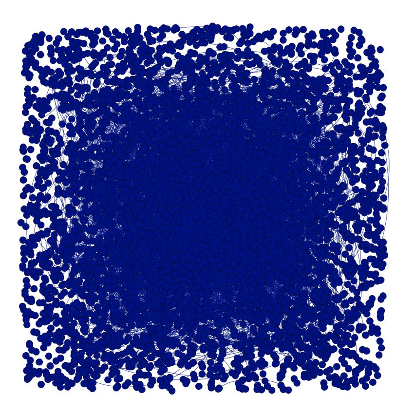
3

Fig. 1 An example of an interesting subgraph. Tweets on Indian politics form a sparse center in a dense periphery (separately
shown in the top right). The bottom two figures show the hashtag distribution of the center and the degree distribution of the
center (log scale) respectively.

   A serious limitation of the above class of work is            graphs whose connectivity properties (e.g., the average
that the interestingness criteria does not take into ac-         degree of a vertices) are distinctly different from an “ex-
count node content (resp. edge content) which may be             pected” background graph. This approach uses a con-
present in a property graph data model (Angles, 2018)            strained optimization problem that maximizes an ob-
where nodes and edges have attributes. (Bendimerad,              jective function over the information content (IC) and
2019) presents several discovery algorithms for graphs           the description length (DL) of the desired subgraph
with vertex attributes and edge attributes. They per-            pattern.
form both structure-based graph clustering and sub-                  Our work is conceptually most inspired by (Bendimerad
space clustering of attributes to identify interesting (in       et al., 2019) that explores the subjective interestingness
their domain “anomalous”) subgraphs.                             problem for attributed graphs. Their main contribution
    On the “subjective” side of the interestingness prob-        centers around CSEA (Cohesive Subgraph with Excep-
lem, one approach considers interesting subgraphs as a           tional Attributes) patterns that inform the user that a
subgraph matching problem (Shan et al., 2019). Their             given set of attributes has exceptional values through-
general idea is to compute all matching subgraphs that           out a set of vertices in the graph. The subjective inter-
satisfy a user the query and then ranking the results            estingness is given by
based on the rarity and the likelihood of the associa-
tions among entities in the subgraphs. In contrast (Adri-
aens et al., 2019) uses the notion of “subjective inter-                                        IC(U, S)
estingness” which roughly corresponds to finding sub-                               S(U, S) =
                                                                                                 DL(U )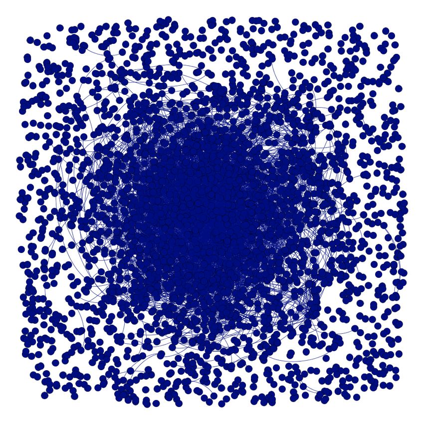
4

where U is a subset of nodes and S is a set of restric-          We realistically assume that the inverse of these map-
tions on the value domains of the attributes. The sys-           pings can be computed, i.e., if v1 , v2 ∈ V are terms, we
tem models the prior beliefs of the user as the Maxi-            can perform a contains−1 (v1 ∧ ¬v2 ) operation to yield
mum Entropy distribution subject to any stated prior,            all posts that used v1 but not v2 .
beliefs the user may hold about the data (e.g., the dis-             The AWESOME information system allows users
tribution of an attribute value). The information con-           construct derived or computed edge types depending
tent IC(U, S) of a CSEA pattern (U, S) is formalized             on the specific discovery problem they want to solve.
as negative of the logarithm of the probability that the         For example, they can construct a standard hashtag
pattern is present under the background distribution.            co-occurrence graph using a non-recursive aggregation
The length of a description of U is the intersection of all      rule in Datalog (Consens and Mendelzon, 1993):
neighborhoods in a subset X ⊆ N (U ), along with the
set of “exceptions”, vertices are in the intersection but        HC(h1 , h2 , count(p)) ←−
not part of U . However, we have a completely different,                              p ∈ P, h1 ∈ H, h2 ∈ H
more database-centric formulation of the background                                   uses(p, h1 ), uses(p, h2 )
and the user’s beliefs.
                                                                 We interpret HC(h1 , h2 , count(p)) as an edge between
                                                                 nodes h1 and h2 and count(p) as an attribute of the
                                                                 edge. In our model, a computed edge has the form:
3 The Problem Setup                                              ET (Nb , Ne , B̄) where ET is the edge type, Nb , Ne are
                                                                 the tail and head nodes of the edge, and B̄ designates a
3.1 Data Model                                                   flat schema of edge properties. The number of such com-
                                                                 puted edges can be arbitrarily large and complex for
Our abstract model social media data takes the form of           different subgraph discovery problems. A more complex
a heterogeneous information network (an information              computed edge may look like: U M U HD(u1 , u2 , mCount, d, h),
network with multiple types of nodes and edges), which           where an edge from u1 to u2 is constructed if user u1
we view as a temporal property graph G. Let N be the             creates a post that contains hashtag h, and mentions
node set and E be the edge set of G. N can be viewed as          user u2 a total number of mCount times on day d. Note
a disjoint union of different subsets (called node types)        that in this case, hashtag h is a property of edge type
– users U , posts P , topic markers (e.g., hastags) H,           U M U HD and is not a topic marker node of graph G.
term vocabulary V (the set of all terms appearing in
a corpus), references (e.g., URLs) R(τ ), where τ repre-
sents the type of resource (e.g., image, video, web site         3.2 Specifying User Knowledge
. . .). Each type of node have a different set of proper-
ties (attributes) Ā(.). We denote the attributes of U as        Since the discovery process is query-driven, the system
Ā(U ) = a1 (U ), a2 (U ) . . . such that ai (U ) is the i-the   has no a priori information about the user’s interests,
attribute of U . An attribute of a node type may be              prior knowledge and expectations, if any, for a specific
temporal – a post p ∈ P may have temporal attribute              discovery task. Hence, given a data corpus, the user
called creationDate. Edges in this network can be di-            needs to provide this information through a set of pa-
rectional and have a single edge type. The following is          rameterized queries. We call these queries “heteroge-
a set of base (but not exhaustive) edge types:                   neous” because they can be placed on conditions on any
                                                                 arbitrary node (resp. edge) properties, network struc-
−   writes: U 7→ P
                                                                 ture and text properties of the graph.
−   uses: P 7→ H
−   mentions: P 7→ U maps a post p to a user u if u              User Interest Specification. The discovery process
    mentioned in p                                               starts with the specification of the user’s universe of
−   repostOf: P 7→ P maps a post p2 to a post p1 if p2 is        discourse identified with a query Q0 . We provide some
    repost of p1 . This implies that ts(p2 ) < ts(p1 ) where     illustrative examples of user interest with queries of in-
    ts is the timestamp attribute                                creasing complexity.
−   replyTo/comment: P 7→ P maps a post p2 to a post             Example 1. “All tweets related to COVID-19 between
    p1 if p2 is a reply to p1 . This implies that ts(p2 ) <      06/01/2020 and 07/31/2020 that refer to Hydroxychloro-
    ts(p1 ) where ts is the timestamp attribute                  quine”. In this specification, the condition “related to
−   contains: P 7→ V × N where N is the set of natural           COVID-19” amounts to finding tweets containing any
    numbers and represents the count of a token v ∈ V            k terms from a user-provided list, and the condition on
    in a post p ∈ P                                              “Hydroxychloroquine” is expressed as a fuzzy search.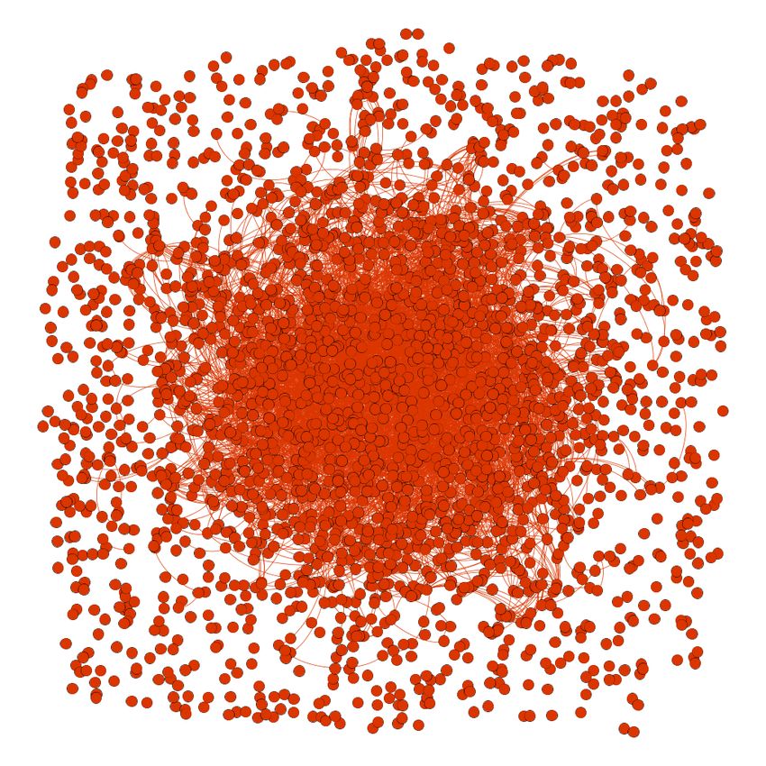
5

                                                             Clearly, we can assert that C(p) is a connected graph
                                                             and that N (p) @g C(p) where @g denotes a subgraph
                                                             relationship.

                                                             Definition 3 (Initial Background Graph.) The ini-
                                                             tial background graph G0 is a merger of all conversa-
                                                             tion contexts C(pi ), pi ∈ P0 , together with all computed
                                                             edges induces the nodes of ∪i C(pi )

                                                             The initial background graph itself can be a gateway to
                                                             finding interesting properties of the graph. To illustrate
Fig. 2 Hydroxychloroquine and COVID related Hashtags         this based on the graph obtained from our Example
                                                             2. Figure 3 presents two views of the #ados cluster of
                                                             hashtags from January 2021. The left chart shows the
Figure 2 shows the top hashtags related to this search       time vs. count of the hashtags while the right chart
– note that the hashtag co-occurrence graph around           shows the dominant hashtags of the same period in this
COVID-19 and hyroxychloroquine includes “FakeNews-           cluster. The strong peak in the timeline, was due to an
Media”.                                                      intense discussion, revealed by topic modeling, on the
Example 2. “All tweets from users who mention Trump          creation of an office on African American issues. The
in their user profile and Fauci in at least n of their       occurrence of this peak is interesting because most of
tweets”. Notice that this query is about users with a        the social media conversation in this time period was
certain behavioral pattern – it captures all tweets from     focused on the Capitol attack on January 6.
users who have a combination of specific profile features        Given the G0 graph,we discover subgraphs Si ⊂ Go
and tweet content.                                           whose content and structure are distinctly different that
Example 3. “All tweets from users U1 whose tweets            of G0 . However, unlike previous approaches, we ap-
appear in hashtag-cooccurrence in the 3 neighborhood         ply a generate-and-test paradigm for discovery. The
around #ados is used together with all tweets of users       generate-step (Section 4) uses a graph cube like (Zhao
U2 who belong to the user-mention-user networks of           et al., 2011) technique to generate candidate subgraphs
these users (i.e., U1 ) ”, where #ados refers to “Ameri-     that might be interesting and the test-step (Section
can Descendant of Slaves”, which represents an African       5.2) computes if (a) the candidate is sufficiently dis-
American cause.                                              tinct from the G0 , and (b) the collection of candidates
The end result of Q0 is a collection of posts that we        are sufficiently distinct from each other.
call the initial post set P0 . Using the posts in P0 , the
                                                             Subgraph Interestingness. For a subgraph Si to be
system creates a background graph as follows.
                                                             considered as a candidate, it must satisfy the following
Initial Background Graph. The initial background             conditions.
graph G0 is the graph derived from P0 over which the         C1. Si must be connected and should satisfy a size
discovery process runs. However, to define the initial       threshold θn , the minimal number of nodes.
graph, we first develop the notion of a conversation.        C2. Let Aij (resp. Bik ) be the set of local properties
                                                             of node j (resp. edge k) of subgraph Si . A property is
Definition 1 (Semantic Neighborhood.) N (p), the             called “local” if it is not a network property like vertex
semantic neighborhood of a post p is the graph connect-      degree. All nodes (resp. edges) of Si must satisfy some
ing p to instances of U ∪ H ∪ P ∪ V that directly relates    user-specified predicate φN (resp. φE ) specified over Aij
to p.                                                        (resp. Bik ). For example, a node predicate might re-
                                                             quire that all “post” nodes in the subgraph must have
Definition 2 (Conversation Context.) The conver-
                                                             a re-post count of at least 300, while an edge predicate
sation context C(p) of post p is a subgraph satisfying
                                                             may require that all hashtag co-occurrence relation-
the following conditions:
                                                             ships must have a weight of at least 10. A user defined
1. P1 : The set of posts reachable to/from p along the       constraint on the candidate subgraph improves the in-
   relationships repostOf, replyTo belong to C(p).           terpretability of the result. Typical subjective interest-
2. P2 : The union of posts in the semantic neighborhood      ingness techniques (van Leeuwen et al., 2016; Adriaens
   of P1 belong to C(p).                                     et al., 2019) use only structural features of the network
3. E: The induced subgraph of P1 ∪ P2 belong to C(p)         and do not consider attribute-based constraints, which
4. Nothing else belongs to C(p).                             limits their pragmatic utility.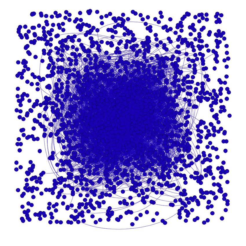
6

Fig. 3 Two views of the #ados cluster of hashtags

C3. For each text-valued attribute a of Aij , let C(a)        value of the grouping attributes, and then applies the
be the collection of the values of a over all nodes of        aggregation function to the list. Thus, the result of the
Si , and D(C(a)) is a textual diversity metric computed       groupby operation is a single aggregated value for each
over C(a). For Si to be interesting, it must have at          distinct cross-product value of grouping attributes.
least one attribute a such that D(C(a)) does not have
the usual power-law distribution expected in social net-          To apply this operation to a social network graph,
works. Zheng et al (Zheng and Gupta, 2019) used vocab-        we recognize that there are two distinct ways of defin-
ulary diversity and topic diversity as textual diversity      ing the “grouping-object”.
measures.                                                     (1) Node properties can be directly used just like in
                                                              the relational case. For example, for tweets a grouping
                                                              condition might be getDate (Tweet.created at) ∧
4 Candidate Subgraph Generation                               bin(Tweet.favoriteCount, 100), where the getDate
                                                              function extracts the date of a tweet and the bin func-
Section 3.2 describes the creation of the initial back-       tion creates buckets of size 100 from the favorite count
ground graph G0 that serves as the domain of discourse        of each tweet.
for discovery. Depending on the number of initial posts       (2) The grouping-object is a subgraph pattern. For ex-
P0 resulting form the initial query, the size of G0 might     ample, the subgraph pattern
be too large – in this case the user can specify followup     (:tweet{date})-[:uses]->(:hashtag{text}) (P1)
queries on G0 to narrow down the scope of discovery.          states that all ”tweet” nodes having the same posting
We call this narrowed-down graph of interest as G0 – if       date, together with every distinct hashtag text will be
no followup queries were used, G0 = G0 . The next step        placed in a separate group. Notice that while (1) pro-
is to generate some candidate subgraphs that will be          duces disjoint tweets, (2) produces a “soft” partitioning
tested for interestingness.                                   on the tweets and hashtags due to the many-to-many
Node Grouping. A node group is a subset of nodes(G0 )         relationship between tweets and hashtags.
where all nodes in a group have some similar property.        In either case, the result is a set of node groups, desig-
We generalize the groupby operation, commonly used            nated here as Ni . For example, the grouping pattern P1
in relational database systems, to heterogeneous infor-       expressed in a Cypher-like syntax (Francis et al., 2018)
mation networks. To describe the generalization, let us       (implemented in the Neo4J graph data management
assume R(A, B, C, D, . . .) is a relation (table) with at-    system) states that all tweets having the same posting
tributes A, B, C, D, . . . A groupby operation takes as in-   date, together with every distinct hashtag text will be
put (a) a subset of grouping attributes (e.g. A, B), (b) a    placed in a separate group. Notice that this process pro-
grouped attribute (e.g., C) and (c) an aggregation func-      duces a “fuzzy” partitioning on the tweets and hashtags
tion (e.g., count). The operation first computes each         due to the many-to-many relationship between tweets
distinct cross-product value of the grouping attributes       and hashtags. Hence, the same tweet node can belong
(in our example, A × B) and creates a list of all values      to two different groups because it has multiple hash-
of the grouped attribute corresponding to each distinct       tags. Similarly, a hashtag node can belong to multiple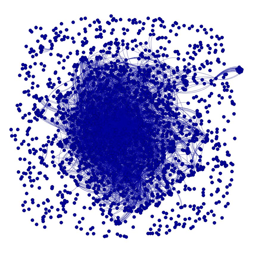
7

groups because tweets from different dates may have                 able, we find a∗, the maximum curvature (elbow)
used the same hashtag. While the grouping condition                 point of f (A) numerically (Antunes et al., 2018).
specification language can express more complex group-           ◦ We compute A0 , the values of attribute A to the
ing conditions, in this paper, we will use simpler cases            left of a∗ for all attributes and choose the at-
to highlight the efficacy of the discovery algorithm. We            tribute where the cardinality of A0 is maximum.
denote the node set in each group as Ni .                           In other words, we choose attributes which have
Graph Construction. To complete the groupby oper-                   the highest number of pre-elbow values.
ation, we also need to specify the aggregation function       – We adopt a similar strategy for subgraph patterns.
                                                                             L
in addition to the grouping-object and the grouped-             If T1 (ai ) −→ T2 (bj ) is an edge where T1 , T2 are node
object. This function takes the form of a graph con-            labels, ai , bj are node properties and L is an edge
struction operation that constructs a subgraph Si by            label, then ai and bj will be selected based on the
expanding on the node set Ni . Different expansion rules        conditions above. Since the number of edge labels is
can be specified, leading to the formation of different         fairly small in our social media data, we will evalu-
graphs. Here we list three rules that we have found fairly      ate the estimated cardinality of the edge for all such
useful in practice.                                             triples and select one with the lowest cardinality.
G1. Identify all the tweet nodes in Ni . Construct a
relaxed induced subgraph of the tweet-labeled nodes in
Ni . The subgraph is induced because it only uses tweets      5 The Discovery Process
contained within Ni , and it is relaxed because contains
all nodes directly associated with these tweet nodes,         5.1 Measures of for Relative Interestingness
such as author, hashtags, URLs, and mentioned-users.
G2. Construct a mention network from within the tweet         We compute the interestingness of a subgraph S in ref-
nodes in Ni – the mention network initially connects all      erence to a background graph Gb (e.g., G0 ), and con-
tweet and user-labeled nodes. Extend the network by           sists of a structural as well as a content component. We
including all nodes directly associated with these tweet      first discuss the structural component. To compare a
nodes.                                                        subgraph Si with the background graph, we first com-
G3. A third construction relaxes the grouping con-            pute a set of network properties Pj (see below) for
straint. We first compute either G1 or G2, and then           nodes (or edges) and then compute the frequency dis-
extend the graph by including the first order neighbor-       tribution f (Pj (Si )) of these properties over all nodes
hood of mentioned users or hashtags. While this clearly       (resp. edges) of (a) subgraphs Si , and (b) the refer-
breaks the initial group boundaries, a network thus           ence graph (e.g., G0 ). A distance between f (Pj (Si ))
constructed includes tweets of similar themes (through        and f (Pj (Gb )) is computed using Jensen–Shannon di-
hashtags) or audience (through mentions).                     vergence (JSD). In the following, we use ∆(f1 , f2 ) to
Automated Group Generation. In a practical set-               refer to the JS-divergence of distributions f1 and f2 .
ting, as shown in Section 6, the parameters for node          Eigenvector Centrality Disparity: The testing pro-
grouping operation can be specified by a user, or it          cess starts by identifying the distributions of nodes with
can be generated automatically. Automatic generation          high node centrality between the networks. While there
of grouping-objects is based on the considerations de-        is no shortage of centrality measures in the literature,
scribed below. To keep the autogeneration manageable,         we choose eigenvector centrality (Das et al., 2018) de-
we will only consider single and two objects for at-          fined below, to represent the dominant nodes. Let A =
tribute grouping and only a single edge for subgraph          (ai,j ) be the adjacency matrix of a graph. The eigen-
patterns.                                                     vector centrality xi of node i is given by:
– Since temporal shifts in social media themes and                                      1X
  structure are almost always of interest, the posting                            xi =        ak,i xk
                                                                                        λ
                                                                                           k
  timestamp is always a grouping variable. For our pur-
  poses, we set the granularity to a day by default,          where λ 6= 0 is a constant. The rationale for this choice
  although a user can set it.                                 follows from earlier studies in (Bonacich, 2007; Ruh-
– The frequency of most nontemporal attributes (like          nau, 2000; Yan et al., 2014), who establish that since
  hashtags) have a mixture distribution of double-pareto      the eigenvector centrality can be seen as a weighted sum
  lognormal distribution and power law (Bhattacharya          of direct and indirect connections, it represents the true
  et al., 2020), we will adopt the following strategy.        structure of the network more faithfully than other cen-
   ◦ Let f (A) be distribution of attribute A, and κ(f (A))   trality measures. Further, (Ruhnau, 2000) proved that
      be the curvature of f (A). If A is a discrete vari-     the eigenvector-centrality under the Euclidean norm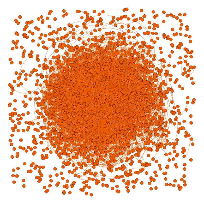
8

can be transformed into node-centrality, a property not        the subgraph) that belong to the cluster. If the number
exhibited by other common measures. Let the distribu-          of posts is greater than a threshold, we compute the
tions of eigenvector centrality of subgraphs A and B           navigability disparity.
be βa and βb respectively, and that of the background
                                                               Propagativeness Disparity: The concept of prop-
graph be βt , then |∆e (βt , βa )| > θ indicates that A is
                                                               agativeness builds on the concept of navigability. Prop-
sufficiently structurally distinct from Gb |∆e (βt , βa )| >
                                                               agativeness attempts to capture how strongly the net-
|∆e (βt , βb )| indicates that A contains significantly more
                                                               work is spreading information through a navigable sub-
or significantly less influential nodes than B.
                                                               graph S. We illustrate the concept with a network con-
Topical Navigability Disparity: Navigability mea-              structed over tweets where a political personality (Sen-
sures ease of flow. If subgraph S is more navigable than       ator Kamala Harris in this example) is mentioned in
subgraph S 0 , then there will be more traffic through         January 2021. The three rows in Figure 10 show the
S compared to S 0 . However, the likelihood of seeing a        network characteristics of the subregions of this graph,
higher flow through a subgraph depends not just on the         related, respectively to the themes of #ados and “black
structure of the network, but on extrinsic covariates like     lives matter” (Row 1), Captiol insurrection (Row 2)
time and topic. So, a subgraph is interesting in terms         and Socioeconomic issues related to COVID-19 includ-
of navigability if for some values of a covariate, its nav-    ing stimulus funding ad business reopening (Row 3). In
igability measure is different from that of a background       earlier work (Zheng and Gupta, 2019), we have shown
subgraph.                                                      that a well known propagation mechanism for tweets is
    Inspired by its application in biology (Seguin et al.,     to add user-mentions to improve the reach of a message
2018), traffic analysis (Scellato et al., 2010), and net-      - hence the user-mention subgraph is indicative of prop-
work attack analysis (Lekha and Balakrishnan, 2020),           agative activity. In Figure 10, we compare the hashtag
we use edge betweenness centrality (Das et al., 2018) as       activity (measured by the Hashtag subgraph) and the
the generic (non-topic) measure of navigability. Let αij       mention activity (size of the mention graph) in these
be the number of shortest paths from node i to j and           three subgraphs. Figure 10 (e) shows a low and fairly
αij (k) is the number of paths passes through the edge         steady size of the user mention activity in relation to the
k. Then the edge-betweenness centrality is                     hashtag activity on the same topic, and these two indi-
                                                               cators are not strongly correlated. Further, Figure 10 (f)
                              X αij (k)
                 Ceb (k) =                                     shows that the mean and standard deviation of node de-
                                 αij                           gree of hashtag activity are fairly close, and the average
                             (i,j)∈V
                                                               degree of user co-mention (two users mentioned in the
By this definition, the edge betweenness centrality is the     same tweet) graph is relatively steady over the period of
portion of all-pairs shortest paths that pass through an       observation – showing low propagativeness. In contrast,
edge. Since edge betweenness centrality of edge e mea-         Row 1 and Row 2 show sharper peaks. But the curve
sures the proportion of paths that passes through e,           in Figure 10 (c) declines and has low, uncorrelated user
a subgraph S with a higher proportion of high-valued           mention activity. Hence, for this topic although there is
edge betweenness centrality implies that S may be more         a lot of discussion (leading to high navigability edges),
navigable than Gb or another subgraph S 0 of the graph,        the propagativeness is quite low. In comparison, Figure
i.e., information propagation is higher through this sub-      10 (a) shows a strong peak and a stronger correlation
graph compared to the whole background network, for            be the two curves indicating more propagativeness. The
that matter, any other subgraph of network having a            higher standard deviation in the co-mention node de-
lower proportion of nodes with high edge betweenness           gree over time (Figure 10 (b)) also shows the making
centrality. Let the distribution of the edge betweenness       of more propagation around this topic compared to the
centrality of two subgraphs A and B are c1 and c2 re-          others.
spectively, and that of the reference graph is c0 . Then,          We capture propagativeness using current flow be-
|∆b (c0 , c1 )| < |∆b (c0 , c2 )| means the second subgraph    tweenness centrality (Brandes and Fleischer, 2005) which
is more navigable than the first.                              is based on Kirchoff’s current laws. We combine this
     To associate navigability with topics, we detect topic    with the average neighbor degree of the nodes of S to
clusters over the background graph and the subgraph            measure the spreading propensity of S. The current flow
being inspected. The exact method for topic cluster            betweenness centrality is the portion of all-pairs short-
finding is independent of the use of topical navigabil-        est paths that pass through a node, and the average
ity. In our setting, we have used topic topic modeling         neighbor degree is the average degree of the neighbor-
and dense region detection in hashtag cooccurrence net-        hood of each node. If a subgraph has higher current flow
works. For each topic cluster, we identify posts (within       betweenness centrality plus a higher average neighbor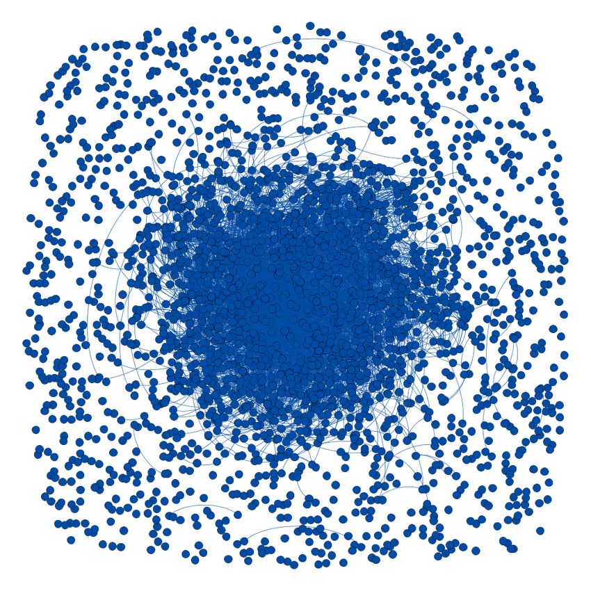
9

degree, the network should have faster communicability.       Algorithm 1: Graph Construction Algorithm
Let αij be the number of shortest paths from node i to         INPUT : Qout Output of the query, L Graph construction
j and αij (n) is the number of paths passes through the         rules, gv grouping variable, thsize is the minimum size of
                                                                the subgraph;
node n. Then the current flow betweenness centrality:          Function gmetrics (Qout , L, groupV ar)
                                                                   G[]← ConstructGraph(Qout , L);
                                X αij (n)                          T ← [];
                  Cnb (n) =                                        for g ∈ G do
                                   αij                                    tα ← ComputeMetrics(g);
                              (i,j)∈V                                     T.push(talpha );
                                                                   end
     Suppose the distribution of the current flow between-         return T
                                                               end
ness centrality of two subgraphs A and B is p1 and p2          Function ComputeMetrics (Graph g)
respectively, and distribution of the reference graph is           m ← [];
                                                                   m.push(eigenV ectorCentrality(g));
pt . Also the distribution of the βn , the average neighbor        ......... m.push(coreN umber(g));
                                                                   return m
degree of the node n, for the subgraph A and B is γ1           end
and γ1 respectively, and the reference distribution is γt .    Function CompareHistograms (List t1 , List x2 )
                                                                   sg ← cut2bin(x2 , binedges );
If the condition                                                   binedges ← getBinEdges(x2 );
                                                                   tg ← cut2bin(t1 , binedges );
                                                                   βjs ← distance.jensenShannon(tg , sg );
      ∆(pt , p1 ) ∗ ∆(γt , γ1 ) < ∆(pt , p2 ) ∗ ∆(γt , γ2 )        ht ← histogram(tg , sg , binedges );
                                                                   return βjs , ht , binedges ;
holds, we can conclude that subgraph B is a faster             end
propagating network than subgraph A. This measure
is of interest in a social media based on the obser-
vation that misinformation/disinformation propagation         Algorithm 2: Graph Discovery Algorithm
groups either try to increase the average neighbor de-         Input: Set of all subgraphs divergence σ
gree by adding fake nodes or try to involve influential        Output: Feature vectors v1 , v2 , v3 , List for re-partition
                                                                         recommendations l
nodes with high edge centrality to propagate the mes-          ev : eigenvector centrality;
sage faster (Besel et al., 2018).                              ec : edge current flow betweenness centrality;
                                                               nc : current flow betweenness centrality;
                                                               µ : core number;
Subgroups within a Candidate Subgraph: The                     z : average neighbor degree;
purpose of the last metric is to determine whether a           Function discover (σ)
                                                                    for any two set of divergence from σ1 ans σ2 do
candidate subgraph identified using the previous mea-                   if σ2 (ev) > σ1 (ev) then
sures need to be further decomposed into smaller sub-                        v1 (σ2 ) = v1 (σ2 ) + 1;
                                                                             if σ2 (ec) > σ1 (ec) then
graphs. We use subgraph centrality (Estrada and Rodriguez-                        v2 (σ2 ) = v2 (σ2 ) + 1;
                                                                                  if (σ2 (nc) + σ2 (µ)) > (σ1 (ec) + σ2 (µ))
Velazquez, 2005) and coreness of nodes as our metrics.                              then
The subgraph centrality measures the number of sub-                                    v3 (σ2 ) = v3 (σ2 ) + 1;
                                                                                  end
graphs a vertex participates in, and the core number                              if (σ2 (sc) + σ2 (z)) > (σ1 (sc) + σ2 (z))
of a node is the largest value k of a k-core containing                             then
                                                                                       l(σ2 ) = 1;
that node. So a subgraph for which the core number                                end
and subgraph centrality distributions are right-skewed                       end
                                                                        end
compared to the background subgraph are (i) either                  end
split around high-coreness nodes, or (ii) reported to the      end
user as a mixture of diverse topics. The node grouping,
per-group subgraph generation and candidate subgraph
identification process is presented in Algorithm 1. In
the algorithm, function cut2bin extends the cut func-     of the first three lists contains one specific factor of
tion, which compares the histograms of the two dis-       interestingness of the subgraph. The most interesting
tributions whose domains (X-values) must overlap, and     subgraph should present in all three vectors. If the sub-
produces equi-width bins to ensure that two histograms    graph has many cores and is sufficiently dense, then
(i.e., frequency distributions) have compatible bins.     the system considers the subgraph to be uninterpretable
                                                          and sends it for re-partitioning. Therefore, the fourth
                                                          list contains the subgraph that should partition again.
5.2 The Testing Process                                   Currently, our repartitioning strategy is to take subsets
                                                          of the original keyword list provided by the user at the
The discovery algorithm’s input is the list of divergence beginning of the discovery process to re-initiate the dis-
values of two candidate sets computed against the same    covery process for the dense, uninterpretable subgraph.
reference graph. It produces four lists at the end. Each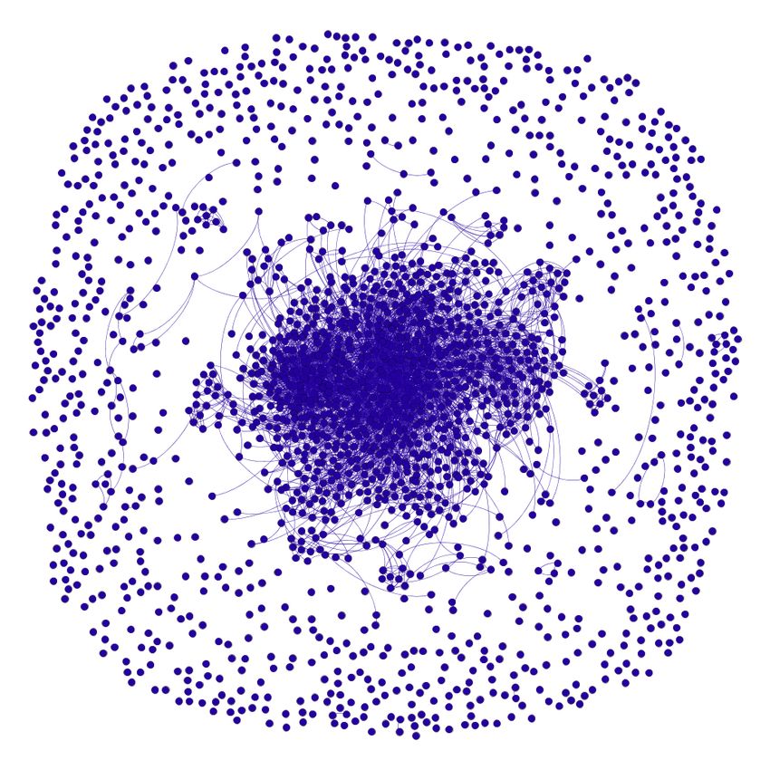
10

Fig. 4 #ADOS and Black Lives Matter                          Fig. 5 AVG Degree Distributions and Std Dev

Fig. 6 Insurrection and Capitol Attack                       Fig. 7 AVG Degree Distributions and Std Dev

Fig. 8 Socioeconomic Issues During COVID-19                  Fig. 9 AVG Degree Distributions and Std Dev
Fig. 10 Various Metrics for Daily Partitioned Hashtag co-occurrences and User mentioned Graph from the Political Personalty
Dataset. Q0 retrieves tweets where Kamala Harris is mentioned in a hashtag, text body or user mention.

The output of each metric produces a value for each            tension of a standard cut function, which compares the
participant node of the input. However, to compare             histograms of the two distributions whose domains (X-
two different candidates, in terms of the metrics men-         values) must overlap. The cut function accepts as input
tioned above, we need to convert them to comparable            a set of set of node property values (e.g., the central-
histograms by applying a binning function depending            ity metrics), and optionally a set of edge boundaries
on the data type of the grouping function.                     for the bins. It returns the histograms of distribution.
Bin Formation (cut2bin): Cut is a conventional opera-          Using the cut, first, we produce n equi-width bins from
tor (available with R, Matlab, Pandas etc. ) segments          the distribution with the narrower domain. Then we ex-
and sorts data values into bins. The cut2bin is an ex-         tract bin edges from the result and use it as the input
11

bin edges to create the wider distribution‘s cut. This        quantitative summary on the three data sets. We used
enforces the histograms to be compatible. In case one         a set of subqueries to find subsets from each of our
of the distribution is known to be a reference distribu-      datasets. These subqueries are temporal, and represent
tion (distribution from the background graph) against         trending terms that stand for the emerging issues. For
which the second distribution is compared, we use the         the first two datasets, we used three themes to con-
reference distribution for equi-width binning and bin         struct the background graphs: a) capitol attack and
the second distribution relative to the first.                insurrection, b) Black Lives Matter and ADOS move-
The CompareHistograms function uses the cut2bin               ment, and c) American economic crisis. and recovery
function to produce the histograms, and then computes         efforts. For the vaccine data set, we selected two subsets
the JS Divergence on the comparable histograms. The           of posts, one for vaccine-related concerns, anti-vaccine
CompareHistograms function returns the set of diver-          movements, and related issues, and the second for covid
gence values for each metric of a subgraph, which is          testing and infection-related issues. The vaccine data
the input of the discovery algorithm. The function re-        set is larger, and the content is more diverse than the
quires the user to specify which of the compared graphs       first two. All the data sets are publicly available from
should be considered as a reference – this is required        The Awesome Lab 1
to ensure that our method is scalable for large back-
                                                                  In the experiments, we constructed two subgraphs
ground graphs (which are typically much larger than
                                                              from each subquery. The first is the “hashtag co-occurrence”
the interesting subgraphs). If the background graph is
                                                              graph, where each hashtag is a node, and they are con-
very large, we take several random subgraphs from this
                                                              nected through an edge if they coexist in a tweet. The
graph to ensure they are representative before the ac-
                                                              second is the “user co-mention” graph, where each user
tual comparisons are conducted. To this end, we adopt
                                                              is a node, and there is an edge between two nodes if a
the well-known random walk strategy.
                                                              tweet mentioned them jointly. Intuitively, the hashtag
In the algorithm v1 , v2 and v3 are the three vectors
                                                              co-occurrence subgraph captures topic prevalence and
to store the interestingness factors of the subgraphs,
                                                              propagation, whereas the co-mention subgraph captures
and l is the list for repartitioning. For two subgraphs, if
                                                              the tendency to influence and propagate messages to a
one of them qualified for v1 means, the subgraph con-
                                                              larger audience. Our goal is to discover surprises (and
tains higher centrality than the other. In that case, it
                                                              lack thereof) in these two aspects for our data sets.
increases the value of that qualified bit in the vector
by one. Similarly, it increases the value of v2 by one,           We note that the dataset chosen is from a month
if the same candidate has high navigability. Finally, it      where the US experienced a major event in the form
increases the v3 , if it has higher propagativeness. The      of the Capitol Attack, and a new administration was
algorithm selects the top-k scores of candidates from         sworn in. This explains why the number of tweets in
each vector, and marks them interesting.                      “Capitol Attack” subgraph is high for both politicians
                                                              in this week, and not surprisingly it is also the most
                                                              discussed topic as evidenced by the high average node
6 Experiments
                                                              degree. Therefore, this “selection bias” sets our expec-
                                                              tation for subjective interestingness – given the specific
6.1 Data Sets
                                                              week we have chosen, this issue will dominate most so-
Data sets used for the experiments are tweets collected       cial media conversations in the USA. We also observe
using the Twitter Streaming API using a set of domain-        the low ratio of the number of unique nodes to the num-
specific, hand-curated keywords. We used three data           ber of tweets, signifying the high number of retweets,
sets, all collected between the 1st and the 31st of Jan-      that signals a form of information propagation over the
uary, 2021. The first two sets are for political person-      network. The propagativeness of the network during
alities. The Kamala Harris data set was collected by          this eventful week is also evidenced by the fact that the
using variants of Kamala Harris’s name together with          unique node count of a co-mention network is almost
her Twitter handle and hashtags constructed from her          75% - 88% higher on average compared to the hashtag
name. The second data set was similarly constructed           co-occur network of the same class. In Section 6.3, we
for Joe Biden. The third data set was collected during        show how our interestingness technique performs in the
the COVID-19 pandemic. The keywords were selected             face of this dataset.
based on popularly co-occurring terms from Google Trends.
We selected the terms manually to ensure that they are
related to the pandemic and vaccine related issues (and    1
                                                              https://code.awesome.sdsc.edu/awsomelabpublic/datasets/int-
not, for example, partisan politics). Table 1 presents a  springer-snam/)
12
Table 1 Dataset Descriptions
Total
Sub Network Total Unique Unique Self Avg
Data Set Collection Density
Query Type Tweets nodes edges Loop Degree
Size
Kamala Capitol Hashtag
12469480 164397 1398 7801 16 0.0025 4.3
Harris Attack co-occur
user
164397 8012 48604 87 0.00012 3.19
co-mention
Hashtag
#ADOS 158419 3671 10738 29 0.0015 5.8
co-occur
user
158419 30829 39865 49 8.3 2.5
co-mention
Economic Hashtag
36678 1278 1828 4 0.0022 2.8
Issues co-occur
user
36678 6971 11584 19 0.0004 3.4
co-mention
Capitol Hashtag
Joe Biden 45258151 676898 7728 21422 50 0.00071 5.49
Attack co-occur
user
676898 82046 101646 130 3.0146 2.473
co-mention
Hashtag
#ADOS 183765 3007 11008 29 0.002 3.85
co-occur
user
158419 29547 40932 56 9.3 2.7
co-mention
Economic Hashtag
138754 2961 5733 10 0.0013 3.87
Issues co-occur
user
138754 21417 19691 23 8.5 1.83
co-mention
Vaccine Hashtag
Vaccine 24172676 1000000 18809 24195 44 2.52 2.5
Anti-vax co-occur
user
1000000 203211 41877 46 2.02 0.4
co-mention
Hashtag
Covid Test 1000000 26671 45378 69 0.00012 3.4
co-occur
user
1000000 188761 83656 109 4.67 0.886
co-mention
hashtag
economy 917890 3002 4395 9 0.0009 2.9
co-occur
user
917890 20590 8528 13 4.023 0.8
co-mention
6.2 Experimental Setup mance optimizations that we implemented are outside
the scope of this paper.
The experimental setup has three steps a) data collec-
tion and archival storage, b)Indexing and storing data, 6.3 Result Analysis
and c) executing analytical pipelines. We used The AWE-
SOME project’s continuous tweet ingestion system that Kamala Harris Network: Figure 29 represents Ka-
collects all the tweets through Twitter 1% REST API mala Harris network. This network is interesting be-
using a set of hand-picked keywords. We used the AWE- cause even in the context of the Capitol Attack and the
SOME Polysotre for indexing, storing, and search the Senate approval of election results, it is dominated by
data. For computation, we used the Nautilus facility #ADOS conversations, not by the other political issues
of the Pacific Research Platform (PRP). Our hardware including economic policies. An analysis of the three in-
configurations are as follows. The Awesome server has teresting measures for this network reveals the follow-
64 GB memory and 32 core processors, the Nautilus ing. The Eigenvector Centrality Disparity for the hash-
has 32 core, and 64 GB nodes. The data ingestion pro- tag network (Figure 23) shows that all the groups gen-
cess required a large memory. Depending on the den- erated by the subqueries are equally distributed, while
sity of the data, this requirement varies. Similarly, cen- the random graph has a higher volume with similar
trality computation is a CPU bounded process. Perfor- trends. Hence, these three subqueries are equally im-13 Fig. 11 Capitol Attack Fig. 12 #ADOS Fig. 13 Economic issues Fig. 14 Top Hashtag Distributions of the Kamala Harris Data set Fig. 15 Capitol Attack Fig. 16 #ADOS Issues Fig. 17 Economic issues Fig. 18 Top Hashtag Distributions of the Joe Biden set portant. However, there are a few spikes on #ADOS 30. The eigenvector centrality disparity shows that the and “Capitol Attack” that indicates the possibility of three subgroups are equally dominated in this network. interestingness. Figure 24 shows that most of the “eco- However, the navigability of the network(figure 31) also nomic issues” has a spike on lower centrality nodes, shows that it is navigable for all three subgraphs. It has but it touches zero with the increased centrality. While two big spikes for “economic issues” and “Capitol at- “Capitol attack” and “#ADOS” has many more spikes tack,” plus many mid-sized spikes for ”#ADOS”. Inter- in different centrality level. Hence, we conclude that this estingly, in the figure 32 the propagativeness shows that network is much more navigable for “Capitol attack” the network is strongly propagative with the economic and “#ADOS”. However, the figure 25 represents Prop- issues and the #ADOS issue, which shows up both in agativeness Disparity, and it is clear from this picture the Capitol Attack and the ADOS subgroups. Inter- that African American issues dominated the conversa- estingly, the “Joe Biden” data’s co-mention network tion here, any subtopic related to it including non-US is- shows more propagativeness than the hashtag co-occur sues like “Tigray” (on Ethiopian genocide) propagated network, which indicates exploring the co-mention sub- quickly in this network. graph will be useful. We also note the occurrence of Biden Network: While the predominance of #ADOS certain complete unexpected topics (e.g., COVIDIOT, issues might still be expected for the Kamala Harris AUSvIND – Australia vs. India) within the ADOS group, data set, we discovered it to be an “dominant enough” while Economic Issues for Biden do not exhibit surpris- subgraph in the Joe Biden data set represented in fig- ing results. ure 36. The eigenvector centrality disparity shows that Vaccine Network In the vacation network, we found the three subgroups are equally dominated in this net- that “economic issues” and “covid tests” are more prop- work. The “Joe Biden” data set represented in figure agative than “vaccine and anti-vaccine” related topics
14
Fig. 19 Vaccine anti-vaccine Issues Fig. 20 COVID-19 Test Fig. 21 Economic issues
Fig. 22 Top Hashtag Distributions of the Vaccine Data set
(Figure 43). The surprising result here is that the “vac- while the core has about the same density as the ran-
cine - anti-vaccine” topics show a strong correlation dom graph. The core periphery separation is much more
with “Economy” in the other two charts. We observe prominent in first three plots of Figure 53. Unlike the
that while the vaccine issues are navigable through the Kamala Harris random graph, Figure 53(d) shows that
network, but this topic cluster is is not very propagative the random graph of this data set itself has a very large
in the network. In contrast, in the co-mention network, dense core and a moderately dense periphery. Among
vaccine and anti-vaccine issues are both very naviga- the three subfigures, the small (but lighter) core of Fig-
ble and strongly propagative. Further, the propagative- ure 53(b) has the maximum difference compared to the
ness in the co-mention network for the Covid-test shows random graph, although we find 53(a) to be conceptu-
many spikes at the different levels, which signifies for ally more interesting. For the vaccine data set, Figure
testing related issues, the network serves as a vehicle of 58 (c)is closest to the random graph showing that most
message propagation and influencing. conversations around the topic touches economic issues,
while the discussion on the vaccine itself (Figure 53(a))
and that of COVID-testing (Figure 53(b)) are more fo-
6.4 Result Validation cused and propagative.
There is not a lot of work in the literature on interest-
ing subgraph finding. Additionally, there are no bench- 7 Conclusion
mark data sets on which our “interestingness finding”
technique can be compared to. This prompted us to In this paper, we presented a general technique to dis-
evaluate the results using a core-periphery analysis as cover interesting subgraphs in social networks with the
indicated earlier in Figure 1. The idea is to demonstrate intent that social network researchers from different do-
that the parts of the network claimed to be interesting mains would find it as a viable research tool. The results
stand out in comparison to the network of a random obtained from the tool will help researchers to probe
sample of comparable size from the background graph. deeper into analyzing the underlying phenomena that
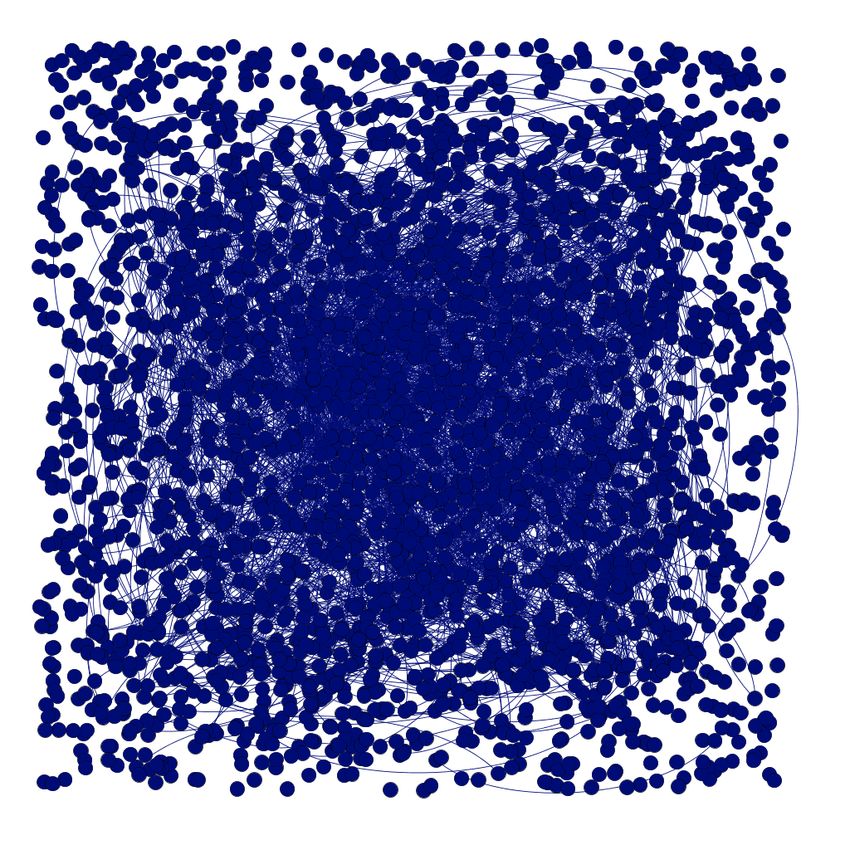
These results are presented in Figures 48, 53, 58. In each leads to the surprising result discovered by the tool.
of these cases, we have shown a representative random While we used Twitter as our example data source, sim-
graph in the rightmost subfigure to represent the back- ilar analysis can be performed on other social media,
ground graph. To us, the large and dense core formation where the content features would be different. Further,
in Figure 48(b) is an expected, non-surprising result. in this paper, we have used a few centrality measures
However, the lack of core formation on Figure 48(c) is to compute divergence-based features – but the system
interesting because it shows while there was a sizeable is designed to plug in other measures as well.
network for economics related term for Kamala Har-
ris, the topics never “gelled” into a core-forming con-
versation and showed little propagation. Figure 48(a)
is somewhat more interesting because the density of
the periphery is far less strong than the random graph15 Fig. 23 Eigenvector Centrality Disparity Hashtag Network Fig. 24 Topical Navigability Disparity Hashtag Network Fig. 25 Propagativeness Disparity Hashtag Network Fig. 26 Eigenvector Centrality Disparity co-mention Network Fig. 27 Topical Navigability Disparity co-mention Network Fig. 28 Propagativeness Disparity co-mention Network Fig. 29 Comparative studies of all sub-queries using the ”Kamala Harris” data set.
16

Fig. 30 Eigenvector Centrality Disparity Hashtag Network     Fig. 31 Topical Navigability Disparity Hashtag Network

Fig. 32 Propagativeness Disparity Hashtag Network            Fig. 33 Eigenvector Centrality Disparity co-mention Network

Fig. 34 Topical Navigability Disparity co-mention Network    Fig. 35 Propagativeness Disparity co-mention Network
Fig. 36 Comparative studies of all sub-queries using the ”Joe Biden” data set.
17

Fig. 37 Eigenvector Centrality Disparity: ”Vaccine” HashtagFig. 38 Topical Navigability Disparity: Vaccine Hashtag Net-
Network                                                    work

Fig. 39 Propagativeness Disparity: ”Vaccine” Hashtag Net-Fig. 40 Eigenvector Centrality Disparity: ”Vaccine” co-
work                                                     mention Network

Fig. 41 Topical Navigability Disparity: ”Vaccine” co-mentionFig. 42 Propagativeness Disparity: ”Vaccine” co-mention Net-
Network                                                     work
Fig. 43 Comparative studies of all sub-queries using the ”Vaccine” data set.
18

Fig. 44 #ADOS                 Fig. 45 Capitol attack        Fig. 46 Economic issues   Fig. 47 Random Graph
Fig. 48 Core and Periphery visualization of ”Kamala Harris” Data set

Fig. 49 #ADOS                 Fig. 50 Capitol attack        Fig. 51 Economic issues   Fig. 52 Random Data
Fig. 53 Core and Periphery visualization of ”Joe Biden” Data set

Fig. 54 Vaccine Issues        Fig. 55 COVID-19 Test         Fig. 56 Economic issues   Fig. 57 Random Graph
Fig. 58 Core and Periphery visualization of the Vaccine Data set
19

Acknowledgements This work was partially supported by       References
NSF Grants #1909875, #1738411. We also acknowledge SDSC
cloud support, particularly Christine Kirkpatrick & Kevin   Adriaens F, Lijffijt J, De Bie T (2019) Subjectively in-
Coakley, for generous help and support for collecting and
managing our tweet collection.                                teresting connecting trees and forests. Data Mining
                                                              and Knowledge Discovery 33(4):1088–1124
                                                            Angles R (2018) The property graph database model.
                                                              In: AMW
                                                            Antonakaki D, Ioannidis S, Fragopoulou P (2018) Uti-
                                                              lizing the average node degree to assess the temporal
                                                              growth rate of twitter. Social Network Analysis and
                                                              Mining 8(1):12
                                                            Antunes M, Gomes D, Aguiar RL (2018) Knee/elbow
                                                              estimation based on first derivative threshold. In:
                                                              Proc. of 4th IEEE International Conference on Big
                                                              Data Computing Service and Applications (Big-
                                                              DataService), IEEE, pp 237–240
                                                            Bendimerad A (2019) Mining useful patterns in at-
                                                              tributed graphs. PhD thesis, Université de Lyon
                                                            Bendimerad A, Mel A, Lijffijt J, Plantevit M, Ro-
                                                              bardet C, De Bie T (2019) Mining subjectively
                                                              interesting attributed subgraphs. arXiv preprint
                                                              arXiv:190503040
                                                            Besel C, Echeverria J, Zhou S (2018) Full cycle analysis
                                                              of a large-scale botnet attack on twitter. In: 2018
                                                              IEEE/ACM International Conference on Advances
                                                              in Social Networks Analysis and Mining (ASONAM),
                                                              IEEE, pp 170–177
                                                            Bhattacharya S, Sinha S, Roy S, Gupta A (2020) To-
                                                              wards finding the best-fit distribution for OSN data.
                                                              J Supercomput 76(12):9882–9900
                                                            Bing Liu, Wynne Hsu, Lai-Fun Mun, Hing-Yan Lee
                                                              (1999) Finding interesting patterns using user expec-
                                                              tations. IEEE Transactions on Knowledge and Data
                                                              Engineering 11(6):817–832, DOI 10.1109/69.824588
                                                            Bonacich P (2007) Some unique properties of eigenvec-
                                                              tor centrality. Soc Networks 29(4):555–564
                                                            Brandes U, Fleischer D (2005) Centrality measures
                                                              based on current flow. In: Annual symposium on
                                                              theoretical aspects of computer science, Springer, pp
                                                              533–544
                                                            Consens MP, Mendelzon AO (1993) Low-complexity
                                                              aggregation in graphlog and datalog. Theoretical
                                                              Computer Science 116(1):95–116
                                                            Das K, Samanta S, Pal M (2018) Study on centrality
                                                              measures in social networks: a survey. Social network
                                                              analysis and mining 8(1):13
                                                            Dasgupta S, Coakley K, Gupta A (2016) Analytics-
                                                              driven data ingestion and derivation in the AWE-
                                                              SOME polystore. In: IEEE International Conference
                                                              on Big Data, Washington DC, USA, IEEE Computer
                                                              Society, pp 2555–2564
                                                            Epasto A, Lattanzi S, Sozio M (2015) Efficient densest
                                                              subgraph computation in evolving graphs. In: Proc.
You can also read