Small Catchment Runoff Sensitivity to Station Density and Spatial Interpolation: Hydrological Modeling of Heavy Rainfall Using a Dense Rain Gauge ...
←
→
Page content transcription
If your browser does not render page correctly, please read the page content below
Article

Small Catchment Runoff Sensitivity to Station Density and
Spatial Interpolation: Hydrological Modeling of Heavy
Rainfall Using a Dense Rain Gauge Network
Clara Hohmann 1,2,*, Gottfried Kirchengast 1,2,3, Sungmin O 2,3,4, Wolfgang Rieger 5 and Ulrich Foelsche 1,2,3

                                          1 Wegener Center for Climate and Global Change (WEGC), University of Graz, 8010 Graz, Austria;
                                            gottfried.kirchengast@uni-graz.at (G.K.), ulrich.foelsche@uni-graz.at (U.F.)
                                          2 FWF-DK Climate Change, University of Graz, 8010 Graz, Austria; sungmin.o@bgc-jena.mpg.de

                                          3 Institute for Geophysics, Astrophysics, and Meteorology/Institute of Physics, University of Graz,

                                            8010 Graz, Austria
                                          4 Department of Biogeochemical Integration, Max Planck Institute for Biogeochemistry, 07745 Jena, Germany

                                          5 Bavarian Environment Agency, 86179 Augsburg, Germany; wolfgang.rieger@lfu.bayern.de

                                          * Correspondence: clara.hohmann@uni-graz.at

                                          Abstract: Precipitation is the most important input to hydrological models, and its spatial variability
                                          can strongly influence modeled runoff. The highly dense station network WegenerNet (0.5 stations
                                          per km2) in southeastern Austria offers the opportunity to study the sensitivity of modeled runoff
                                          to precipitation input. We performed a large set of runoff simulations (WaSiM model) using 16
Citation: Hohmann, C.; Kirchengast,
                                          subnetworks with varying station densities and two interpolation schemes (inverse distance
G.; O, S.; Rieger, W.; Foelsche, U.
Small Catchment Runoff Sensitivity
                                          weighting, Thiessen polygons). Six representative heavy precipitation events were analyzed, plac-
to Station Density and Spatial            ing a focus on small subcatchments (10–30 km2) and different event durations. We found that the
Interpolation: Hydrological               modeling performance generally improved when the station density was increased up to a certain
Modeling of Heavy Rainfall Using a        resolution: a mean nearest neighbor distance of around 6 km for long-duration events and about 2.5
Dense Rain Gauge Network. Water           km for short-duration events. However, this is not always true for small subcatchments. The suffi-
2021, 13, 1381. https://doi.org/          cient station density is clearly dependent on the catchment area, event type, and station distribution.
10.3390/w13101381                         When the network is very dense (mean distance < 1.7 km), any reasonable interpolation choice is
                                          suitable. Overall, the station density is much more important than the interpolation scheme. Our
Academic Editor: Scott Curtis
                                          findings highlight the need to study extreme precipitation characteristics in combination with run-
                                          off modeling to decompose precipitation uncertainties more comprehensively.
Received: 26 March 2021
Accepted: 11 May 2021
                                          Keywords: precipitation variability; extreme events; rain gauge network; hydrological modeling;
Published: 15 May 2021
                                          sensitivity analysis; spatial rainfall resolution; precipitation interpolation
Publisher’s Note: MDPI stays neu-
tral with regard to jurisdictional
claims in published maps and institu-
tional affiliations.                      1. Introduction
                                               Heavy precipitation events can have significant impacts on society and ecosystems
                                          by causing severe floods and landslides. Moreover, such events are intensifying due to
                                          climate change in many areas [1–4]. Hydrological models have served as an important
Copyright: © 2021 by the authors. Li-     tool to assess the impacts of heavy precipitation events on runoff and other hydrological
censee MDPI, Basel, Switzerland.
                                          processes. Since precipitation is the most important input in hydrological models [5–7], it
This article is an open access article
                                          is crucial to understand its uncertainty and how this uncertainty affects the simulated
distributed under the terms and con-
                                          runoff. Assessing the spatial and temporal heterogeneity of precipitation is becoming in-
ditions of the Creative Commons At-
                                          creasingly important, especially with respect to heavy precipitation events [8,9]. Convec-
tribution (CC BY) license (http://crea-
tivecommons.org/licenses/by/4.0/).
                                          tive storm cells with large volumes of precipitation can easily trigger hazards, but the
                                          limited spatial and temporal extent of these cells is associated with huge levels of meas-
                                          urement uncertainty [10]. In addition to the measurement uncertainty of rain gauges, con-
                                          siderable uncertainty can arise when point-level measurements are spatially interpolated

Water 2021, 13, 1381. https://doi.org/10.3390/w13101381                                                               www.mdpi.com/journal/water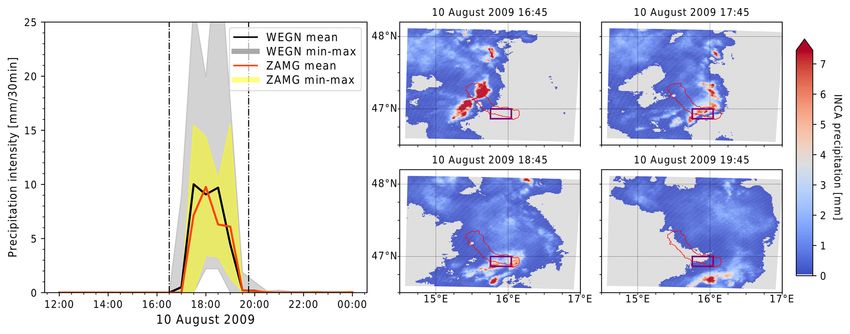
Water 2021, 13, 1381                                                                                            2 of 28

                       to obtain final gridded products [10–13]. Such gridded datasets are crucial in that they
                       allow researchers to collect areal precipitation information within catchment and sub-
                       catchment areas, which can then especially be used in spatially distributed hydrological
                       models. Areal precipitation data can also be derived from radar and satellite-based obser-
                       vations. However, all measurements come with their own uncertainty levels and pros and
                       cons [7,14]. On the one hand, the point measurements are most reliable for quantitatively
                       measuring amounts of precipitation, whereas such measurements often do not provide
                       reliable information about the spatial patterns of heavy precipitation because of the sparse
                       distribution of point measurement sites. On the other hand, radar systems and satellites
                       provide higher spatial resolution data, but the indirect precipitation estimates they pro-
                       vide do not allow the quantitation of specific precipitation amounts [15–21].
                             Despite the availability of remote-sensing data, ground-based precipitation measure-
                       ment tools are still widely used in hydrological modeling [6,22]. Many studies, such as
                       those by Lopez et al. [22], Goovaerts [23], and Zeng et al. [6], pointed out the advantages
                       of dense and regularly distributed precipitation station networks. For many years, re-
                       searchers have analyzed the effect of precipitation station density on hydrological model
                       performance [5,6,12,24–27]. Dong et al. [25] and Xu et al. [27] used a statistical approach
                       to identify the appropriate number of precipitation gauges and the influence of gauge
                       density on the model performance of a lumped model. Both studies found a threshold
                       above which an increase in station density does not lead to better model performance.
                       Such a threshold can also be seen in many other studies [5,6]. Meselhe et al. [26] applied a
                       conceptual and a physically based model to identify the impact of temporally and spa-
                       tially sampling precipitation on runoff predictions (using a highly dense station network).
                       The physically based model was more sensitive to changes in the spatial and temporal
                       resolution of rainfall. A threshold with no significant increase in model performance can
                       also be seen in this case for both models. Huang et al. [12] used a lumped and a distributed
                       hydrological model to study the sensitivity of model performance to spatial rainfall reso-
                       lution. They identified temporal resolution as the most important aspect, observing better
                       model performance at higher temporal resolutions. Many of these studies placed a focus
                       on the model performance and used lumped hydrological models. Here, we focus on the
                       sensitivity of runoff in small subcatchments and report results of a process-based model.
                             When using station data as rainfall input for hydrological models, the spatial inter-
                       polation schemes must also be considered. Many different interpolation options and pos-
                       sibilities have been broadly studied [28–30] including arithmetic mean [12,25,31], Thiessen
                       polygons (TP) [6,26,32], inverse distance weighting (IDW) [13,33–35], and different types
                       of kriging, such as ordinary kriging [8,33,35] or external drift kriging [5,27,33]. The differ-
                       ences between the interpolation schemes are especially pronounced when extreme values
                       are included [30]. Therefore, the selection of interpolation schemes can affect hydrological
                       simulations, especially under heavy rainfall events. Given that our study area has a mod-
                       erate topography with regularly distributed stations [36], we did not expect to obtain
                       added value by using more complex geostatistical methods such as kriging. Therefore, we
                       decided to focus on the two most widely used deterministic interpolation schemes, TP
                       and IDW. We further analyzed the weighting power parameter of the IDW interpolation,
                       which indicates the weight of the surrounding stations. A weighting power of 2 is nor-
                       mally used for IDW interpolations [37] but without making any further considerations
                       [38]. Only a few studies have analyzed the influence of the weighting power on hydrolog-
                       ical model simulations [38,39], while some other studies have focused only on the inter-
                       polated precipitation [37,40].
                             To counteract the uncertainty with respect to spatial and temporal resolution, it is
                       possible to take ground-based measurements from a highly dense station network. In this
                       study, the following research questions were addressed: How many precipitation stations
                       do we need to reliably model runoff during heavy rainfall events? Are there specific fea-
                       tures of small subcatchments to reliably model runoff under heavy rainfall events? How
                       strongly does the interpolation scheme influence runoff results when the precipitation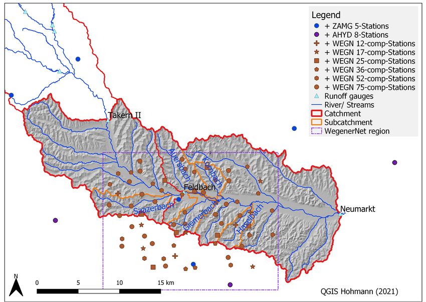
Water 2021, 13, 1381                                                                                            3 of 28

                       station density is the same? The highly dense station network WegenerNet (WEGN)
                       (about 0.5 station per 1 km2 over an area of around 300 km2) in the southeastern Alpine
                       forelands of Austria was used to ask these questions as applied to the Raab catchment and
                       its subcatchment areas. The region is well known for its heavy precipitation events [35,41].
                       Because of the exceptionally dense data coverage, it was possible to analyze the influence
                       of precipitation station densities on runoff in detail. Therefore, we set up the widely used,
                       physically based “Water Flow and Balance Simulation Model” WaSiM [42] and simulated
                       runoff with varying station densities. All subnetworks were simulated using different pre-
                       cipitation interpolation schemes, namely, one TP scheme and three IDW schemes with a
                       weighting power of 1 (IDW1), of 2 (IDW2), and of 3 (IDW3). Previous studies have as-
                       sessed the impact of the station density and interpolation on precipitation data quality,
                       such as mean and extreme rainfall values [43–45]. We go one step further, applying our
                       initial study approach and focus to study the impact of such precipitation uncertainty on
                       hydrologic simulation results, and especially on runoff peaks, using a combination of sta-
                       tion densities and interpolation methods.

                       2. Study Area and Data
                       2.1. Study Area
                             The study area is part of the Raab catchment, an area of southeastern Alpine foreland
                       draining into the Raab river. The Raab river flows from the “Passailer” Alps in the prov-
                       ince of Styria, Austria, at an altitude of around 1150 m.a.s.l. until it joins the Danube river
                       in Hungary. The area covered in this study ranges from the gauging station Takern II/
                       Raab to Neumarkt/Raab, including a total area of around 500 km2 (Figure 1). The gauging
                       station Feldbach/Raab is located between these two stations. Beside the main river Raab,
                       we analyzed five subcatchments (Table 1, Figure 1) with areas of around 10 to 30 km2, all
                       of which are covered by the WEGN. Two subcatchments are located on the northern side
                       of the Raab and three on the southern. Since we did not have measured runoff data for
                       these subcatchments, we implemented pour points in the model directly before they
                       flowed into the Raab river.
                             The total study area is moderately hilly with elevations ranging from 230 to 530 m.
                       The land use is predominately agricultural with some patchy forest areas. The dominant
                       soil texture is sandy loam. The mean annual precipitation is around 850 mm, and the mean
                       annual temperature about 9.5 °C. The study area was chosen because of its vulnerability
                       to heavy/convective precipitation events [41] and climate change [46], as well as the data
                       availability. Since the region has a very dense climate network, the WEGN, which is op-
                       erated by the Wegener Center for Climate and Global Change, University of Graz, Austria
                       [36]. The WEGN has been used to measure precipitation, temperature, humidity, and other
                       variables since early 2007 and includes 150 stations within an area of around 23 × 18 km. All
                       data are quality controlled by the WEGN QC system [36], and additional bias correction
                       is implemented for precipitation data [47].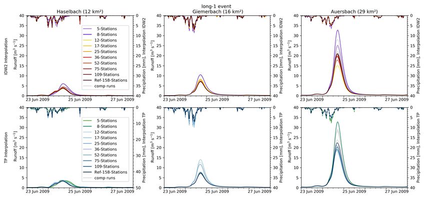
Water 2021, 13, 1381                                                                                                             4 of 28

      Figure 1. Map of the Raab catchment area in southeastern Austria (left), including the full catchment area extending down
      to the runoff gauge Neumarkt/Raab (red line), the focus area (grey area), the subcatchments (orange line), the WegenerNet
      region (violet box), the locations of rain gauge stations (dot symbols), and the runoff gauges (triangle symbols). Inset
      shows a map of Europe; Austria is shown in yellow and the Raab catchment, in red. An enlarged view of the study area
      (right) shows the station subnetworks and subcatchments used in this study.

                                 Table 1. Characteristics of the study catchment area and representative subcatchment areas with
                                 the total basin area of the latter extending up to the gauging station/pour point into the river Raab.

                                                  Catchment                               Area (km2)        Location from Raab
                                         Neumarkt/Raab (total catchment)                     987                     -
                                           Neumarkt/Raab (focus area)                        488                     -
                                         Feldbach/Raab (total catchment)                     689                     -
                                           Feldbach/Raab (focus area)                        190                     -
                                                 Subcatchment                             Area (km2)        Location from Raab
                                                   Auersbach                                 28.9                  north
                                                  Saazerbach                                 27.2                  south
                                                  Giemerbach                                 16.0                  south
                                                   Haselbach                                 12.3                  south
                                                   Kornbach                                  12.2                  north

                                 2.2. Data
                                      To perform hydrological modeling with WaSiM, we need meteorological data for
                                 precipitation, temperature, relative humidity, wind speed, global radiation, and air pres-
                                 sure aggregated at a 30-minute time resolution. Table 2 provides an overview of the max-
                                 imum available number of stations for each parameter, as well as the station source. The
                                 WEGN has a dense station network and a 5-minute time resolution, forming a rectangular
                                 grid due to the comparability to climate models. It is located in the middle of the focus
                                 area around the Feldbach/Raab gauging station, but does not cover the total Raab catch-
                                 ment area. Therefore, we also needed to include data from the Austrian Weather Service
                                 (ZAMG), which has a 15-minute time resolution, and from the Austrian Hydrographic
                                 Service (AHYD), which has a 1- to 15-minute time resolution to properly simulate runoff
                                 (Table 2). In order to run the model only for the focus area, the Takern II/Raab gauging
                                 station was used as an inflow point. Runoff data from the Neumarkt/Raab gauging station
                                 were used for calibration and from the Feldbach/Raab gauging station for cross checks
                                 and further analysis. For precipitation event identification, the Integrated Nowcasting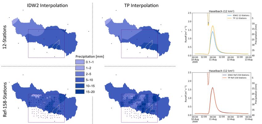
Water 2021, 13, 1381                                                                                             5 of 28

                       through Comprehensive Analysis (INCA) system developed by Haiden et al. [48] was
                       used, which is a multivariable analysis and nowcasting system developed at the ZAMG.

                       Table 2. Catchment attributes and hydrometeorological data used for hydrological modeling with
                       WaSiM with the following sources: HYDROBOD—homogeneous soil and land use grids by
                       Klebinder et al. [49]; LStmk/LBgld—state government offices of the provinces of Styria and Bur-
                       genland; TANALYS—pre-processing tool of the hydrological model WaSiM [42]; WEGN—highly
                       dense station network data version 7.1 [50]; ZAMG—data from the Austrian Weather Service;
                       AHYD—data from the Austrian Hydrographic Service.

                            Catchment Attributes                  Source                       Resolution
                                Land use types                 HYDROBOD                          100 m
                                Soil information               HYDROBOD                          100 m
                                      DEM                      LStmk, LBgld                       10 m
                                 River network                 LStmk, LBgld                         -
                            Geological information             LStmk, LBgld                         -
                            Subcatchments, slope,
                            river width and depth,           TANALYS output                       100 m
                               other information
                             Meteorological Data                   Source                 Number of Stations
                                  Precipitation                    WEGN                         150
                                                                   ZAMG                           5
                                                                   AHYD                          3
                                 Temperature                       WEGN                         150
                                                                   ZAMG                           5
                                                                   AHYD                          3
                              Relative humidity                    WEGN                         150
                                                                   ZAMG                           5
                                                                   AHYD                          3
                                  Wind speed                       WEGN                          12
                                                                   ZAMG                           5
                                 Air pressure                      WEGN                          1
                                                                   ZAMG                           5
                               Global radiation                    ZAMG                           5
                                   Runoff                          AHYD                           3

                             Static attributes are needed in addition to hydrometeorological station data. The dig-
                       ital elevation model (DEM), river network, and geological information were provided by
                       the Austrian state government offices of Styria and Burgenland. The topographic analysis
                       tool (TANALYS) of WaSiM uses the DEM to calculate other required grids, such as flow-
                       time, subcatchments, slope, river width, and depth [42]. Homogeneous soil and land use
                       grids (HYDROBOD) were provided by Klebinder et al. [49] with a resolution of 100 × 100 m
                       in our research area. The HYDROBOD maps were created using the methods cited in
                       Krammer et al. [51]. Maps for every single soil layer (0–20, 20–50, 50–100 cm) and param-
                       eters such as soil texture (percentage of sand, silt, and clay), saturated hydraulic conduc-
                       tivity, Mualem van Genuchten parameters (combinations of residual water content and
                       saturation water content), and soil thickness were used.

                       3. Modeling Approach
                       3.1. Model Setup and Calibration
                            We used the hydrological model WaSiM, which was developed by Schulla [42], at
                       the ETH Zurich in Switzerland for studying climate change in Alpine catchments. WaSiM
                       is a well-established, widely used, distributed, and process-oriented hydrological model.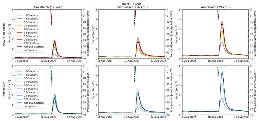
Water 2021, 13, 1381                                                                                             6 of 28

                       It has been used in similar catchments and for many different purposes, such as to perform
                       climate change studies [46,52,53], land use change studies [54,55], and measure opera-
                       tional uses (e.g., at FOEN Switzerland). We focused on a process-oriented model to keep
                       the model uncertainty as small as possible as compared to conceptual models, which are
                       often used for similar precipitation runoff studies [6,12,25]. Using this type of model also
                       allowed us to study ungauged subcatchments within our calibrated catchment area. Fur-
                       thermore, WaSiM had already been successfully applied by Hohmann et al. [46] in the
                       study area to perform a climate change sensitivity study with a low-flow focus.
                             In this study, we used the WaSiM-Richards Version 10.04.07. All modules of WaSiM
                       used are shown in Figure 2. For more information about the modules, see Schulla [42] or
                       the WaSiM user guide by Schulla [56]. The model was set up with a spatial resolution of
                       100 × 100 m and a temporal resolution of 30 min. WaSiM allows the option to internally
                       interpolate the meteorological station data to grids. The evapotranspiration was estimated
                       with the Penman–Monteith equation [57], and the unsaturated zone with the Richards
                       equation, parameterized after van Genuchten [58]. The soil was split up into four calcula-
                       tion layers (0–20, 20–50, 50–100 cm, 1–20 m) with a total depth of 20 m, including the first
                       groundwater layer. By including the data from Klebinder et al. [49], we could include a
                       total of 416 soil parameter combinations in the soil table of WaSiM for our study domain.
                       The final groundwater parameters of the 2D groundwater module were fitted to represent
                       the baseflow quite accurately during the calibration period. Therefore, the saturated hor-
                       izontal conductivity was split up into areas around the river with 1 × 10⁻³ m s−1 and the
                       surrounding hilly areas with 5 × 10⁻⁴ m s−1. Adopting reasonable values, the colmation
                       factor was set to 5 × 10⁻⁵, and the unitless specific storage coefficient to 0.2. In addition to
                       the gridded groundwater parameters, WaSiM was calibrated using four soil module pa-
                       rameters, which influence the shape and volume of the simulated runoff hydrograph
                       when no measured or literature data were available [56]: these were the storage coefficient
                       of the surface runoff kd (shape of the surface runoff hydrograph) and interflow ki (shape
                       of the interflow hydrograph), the drainage density for interflow dr, and a recession con-
                       stant of the soil krec (both of which influence the amount of interflow).
                             The model calibration period was from 1 May to 30 September 2009 with a model
                       spin-up period from 1 November 2007 to 30 April 2009. We calibrated the model only for
                       the extended summer months (May to September), since most of the heavy rainfall events
                       occur during these months in southeastern Styria. The validation periods were the ex-
                       tended summers of 2010 and 2011. The model performance was assessed with the Nash–
                       Sutcliffe model efficiency coefficient (NSE) [59], logarithmic Nash–Sutcliffe efficiency
                       (logNSE), Kling–Gupta efficiency (KGE) [60], and percent bias (PBIAS) [61]. NSE is the
                       most frequently used performance measure in hydrological modelling and places a focus
                       on peak flow [62]. To collect information about the overall flow and especially about the
                       low-flow periods, logNSE was included [46]. KGE provides information about the corre-
                       lation, bias, and variability between the simulations and observed discharge [62]. PBIAS
                       provides the average tendency of the over- and underestimation of the discharge [61].
                             The calibration was mostly performed manually. To obtain a first best-guess of the
                       model parameters, the shuffled complex evolution optimization algorithm developed at
                       the University of Arizona (SCE-UA) [63] was used. The manual calibration was first per-
                       formed with a focus on the efficiency measures and by carrying out a visual comparison
                       of the time series of measured and simulated runoff. Second, since the runoff components
                       such as base flow, interflow, and surface runoff are important in process-based modelling,
                       we visually analyzed the distribution of the runoff components for specific events. Be-
                       cause manual calibration steps were necessary, the model was calibrated with the IDW2
                       interpolation and 158 precipitation stations and was not recalibrated with all different
                       precipitation inputs and interpolation schemes. This approach is considered as appropri-
                       ate, because the deviation between the efficiency measures for all studied cases from those
                       observed in the calibration run was found to be negligible. The deviations observed in the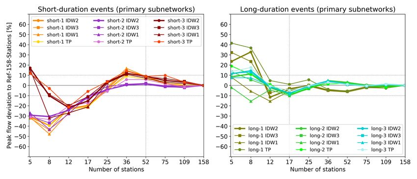
Water 2021, 13, 1381                                                                                             7 of 28

                       calibration/validation period exhibited a maximum deviation of 0.04/0.02 in NSE,
                       0.07/0.13 in logNSE, 0.08/0.04 in KGE, and 11/14% for PBIAS, respectively.
                            The best model performance was obtained with the parameter set of krec = 0.8, dr = 40,
                       kd = 1.5, and ki = 2. This setup resulted in a model performance for the river runoff in the
                       calibration period of summer 2009 with an NSE of 0.80, logNSE of 0.76, KGE of 0.77, and
                       PBIAS of 8%. The validation period of summer 2010 and 2011 resulted in an NSE of 0.63,
                       logNSE of 0.56, KGE of 0.69, and PBIAS of 19%. The observed and simulated runoff for
                       the calibration and validation periods are plotted in Figure A2 in Appendix A.

                       Figure 2. WaSiM model setup, including modules and input datasets used in this study (created
                       after scheme of Schulla [56]). The focus of this study was to evaluate runoff output data (box
                       marked in dark blue) as simulated by WaSiM with various precipitation data resolutions at input
                       (blue box), and using different interpolation schemes (violet box) IDW—inverse distance
                       weighting and TP—Thiessen polygons.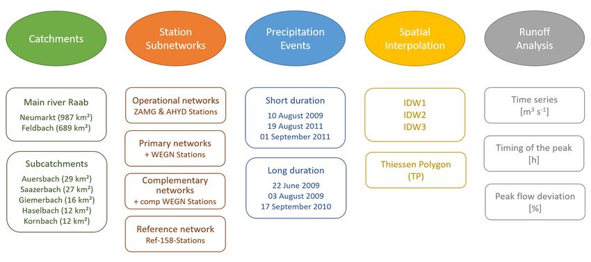
Water 2021, 13, 1381                                                                                                         8 of 28

                                 3.2. Experimental Design
                                      Our study design is visualized in Figure 3 and described in the following sections.

      Figure 3. Overview of the study design with total catchment and subcatchment areas, gauge station subnetworks
      (ZAMG—data from the Austrian Weather Service; AHYD—data from the Austrian Hydrographic Service; WEGN—
      highly dense station network), and full precipitation network (Ref-158-Stations), analyzed short-duration and long-dura-
      tion events, spatial interpolation schemes (inverse distance weighting with power of 1 (IDW1), power of 2 (IDW2) and
      power of 3 (IDW3); Thiessen polygons (TP)) for precipitation input data, and the key runoff output data analyzed.

                                 3.2.1. Selection of Precipitation Station Network Densities
                                      To obtain precipitation input data at various spatial resolutions, we defined subnet-
                                 works (Table 3 and Figure 3) using the 158 stations. The lowest-density network includes
                                 only the five ZAMG stations (5-Stations); the mean nearest neighbor distance is 11.0 km.
                                 This corresponds to an operational meteorological monitoring setup in Austria. The next
                                 subnetwork includes three more stations from the AHYD network (8-Stations). This
                                 would be a typical setup for the operational use of hydrological models.
                                      In addition to the operational setup, precipitation stations from the WEGN are in-
                                 cluded for higher resolution subnetworks. For the main analyses, we defined seven evenly
                                 distributed subnetworks consisting of rain gauges ranging from 12–109 stations (primary
                                 subnetworks in Table 3 and Figure 1). In addition, we defined six complementary subnet-
                                 work cases ranging from 12–75 stations with different actual WEGN stations (Table 3 and
                                 Figure A1 in Appendix A). The spatial uncertainty of the precipitation depends not only
                                 on the number of gauges or station density, but also on their spatial configuration [13].
                                 Therefore, these complementary subnetworks were considered to further investigate the
                                 uncertainty that was related to a given number of pre-defined subnetworks.
                                      All available precipitation stations, 158 in total, served as our reference (Ref-158-Sta-
                                 tions) with a mean nearest neighbor distance of 1.4 km. We assumed that the most accu-
                                 rate areal precipitation information could be obtained from Ref-158-Stations, and there-
                                 fore, we calibrated the model using this setup.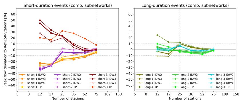
Water 2021, 13, 1381                                                                                               9 of 28

                       Table 3. Precipitation stations of the operational subnetwork cases, the primary subnetwork cases,
                       the complementary subnetwork cases, and the reference subnetwork with the total number of
                       stations per subnetwork, together with the specific station data source (Z: ZAMG, A: AHYD, W:
                       WEGN) and the estimated mean nearest neighbor distance. The distance estimates were calculated
                       with an ArcGIS software tool.

                                           Gauge                        Number                  Mean Nearest
                        Subnetworks
                                     Subnetwork Case              of Stations (Z/A/W)       Neighbor Distance (km)
                        Operational      5-Stations                      5 (5/-/-)                   11.0
                                         8-Stations                      8 (5/3/-)                   10.5
                          Primary       12-Stations                     12 (5/3/4)                    7.2
                                        17-Stations                     17 (5/3/9)                    5.9
                                        25-Stations                    25 (5/3/17)                    4.0
                                        36-Stations                    36 (5/3/28)                    3.2
                                        52-Stations                    52 (5/3/44)                    2.6
                                        75-Stations                    75 (5/3/67)                    2.0
                                        109-Stations                  109 (5/3/101)                  1.7
                       Complementary 12-comp-Stations               12 (5/3/4 comp)                   8.3
                                     17-comp-Stations               17 (5/3/9 comp)                   5.4
                                     25-comp-Stations               25 (5/3/17 comp)                  4.1
                                     36-comp-Stations               36 (5/3/28 comp)                  3.0
                                     52-comp-Stations               52 (5/3/44 comp)                  2.4
                                     75-comp-Stations               75 (5/3/67 comp)                  2.0
                         Reference    Ref-158-Stations                158 (5/3/150)                  1.4

                       3.2.2. Selection of Precipitation Events
                            We selected heavy precipitation events observed with the WEGN during the ex-
                       tended summer (May–September) period in 2009–2014 (see also [11]). We first defined
                       rain events with a minimum inter-event time of 6 h [64,65] and then selected the top 10%
                       of the heaviest rainfall events. Finally, for the case studies, the three most extreme, small-
                       scale, short-duration and the three most extreme, large-scale, long-duration events were
                       selected (see also Figure A3 in Appendix A). The short-duration events were identified as
                       the three events with the strongest peak hour during our study period. The long-duration
                       events were selected as those with the largest total precipitation amount. We additionally
                       conducted a visual inspection of the INCA data across the study area (Figure 4) to check
                       the spatial scales of the selected rainfall events. Table 4 shows a description of the six
                       rainfall events considered in this study.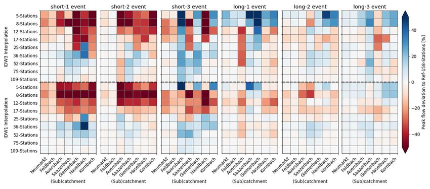
Water 2021, 13, 1381                                                                                                             10 of 28

      Figure 4. Precipitation time series of the “short-1 event” measured at WEGN and ZAMG stations (left panel) throughout
      the WEGN network area (purple box in the four panels on the right). In the panel on the left, “WEGN” shows mean areal
      precipitation computed from the 150 stations (black line) with a min–max range among the stations (gray shaded), while
      “ZAMG” shows mean precipitation (red line) obtained from the 3 ZAMG stations with a min–max range across the sta-
      tions (yellow-shaded). The map sequence in the four panels on the right shows the evolution of the precipitation event as
      revealed by the gridded INCA analysis across the WEGN network (purple box) and the Raab catchment area (red line).

      Table 4. Precipitation events selected for this study and associated key characteristics. The precipitation information indi-
      cated for the events was estimated from WEGN data. The runoff information included the measured peak runoff at the
      total catchment outlet, the Neumarkt/Raab gauging station. The HQ gives a rating if the peak runoff was statistically
      reached or exceeded once per year (HQ1) or once per ten years (HQ10).

                                    Duration           Total Precipitation          Peak Hourly            Peak Runoff
    Event              Start Date                                                                                               HQ
                                      (h)                     (mm)               Precipitation (mm)          (m3 s−1)
    short-1        10 August 2009      4                        34                       19                    107             HQ1
    short-2        19 August 2011      2                        23                       18                     36
Water 2021, 13, 1381 11 of 28
̂( ) = ∙ (1)
with = ⋅ and =∑ follows ∑ =1 (2)
, ,
̂( ) interpolated value at location u.
weight of the observed value at the station j.
observed value at the station j.
, distance to the station j.
weighting-power exponent of the inverse-distance scheme.
In our study, we used the standard weighting power p of 2 (IDW2) as well as the
weighting power p of 1 (IDW1) and of 3 (IDW3) for comparison. The search radius was
set differently for the core WEGN region and the surrounding stations. Since our focus
region was the WEGN region itself, and we do not have such a dense network throughout
the entire catchment area, we maintained a fixed precipitation input for the surrounding
area. So, for the 12-Stations case and onwards, the IDW2 interpolation case with the five
ZAMG and three AHYD stations and a 60 km radius of influence was maintained for the
surrounding area.
The WEGN region (23 × 18 km) was then interpolated with each subnetwork and
interpolation scheme, respectively. A smoothing buffer of 3 km was set, between the
WEGN region and its surroundings. This setup enabled us to change the radius of influ-
ence for the WEGN stations individually without losing important information from the
supporting weather stations. The radius of influence was subsequently set to 20 km for
the 12- and 17-Stations cases and to 10 km for the 25-Stations case and onward so that we
could include all supporting information and still obtain proper information for all loca-
tions.
Using the TP interpolation, the precipitation data collected at the nearest station were
always taken. Each grid cell of the model received information from the nearest station,
and the polygons formed (Thiessen polygons) represent lines of equal distance between
two stations [42]. Hence, TP is a simpler method to apply than IDW, but the former is still
widely used in hydrological modeling [6,26,32].
3.2.4. Runoff Analysis Approach
In our study, we analyzed an event-specific time series of runoff and peak flow de-
viations. The time series are visualized for all events individually, but are combined with
different station network densities and interpolation schemes. For each catchment, inter-
polation method, and event, the peak flow deviation was calculated individually as a per-
cent of the total value. For this purpose, the maximum runoff value was calculated using
the simulation results from every subnetwork case (MAX value); this value was then com-
pared to the maximum runoff value from the full-network reference case (MAX Ref-158-
Stations), which best captures the “true” spatial variability of precipitation in the study
area. This deviation metric is computed as follows:
(MAX value) − (MAX Ref-158-Stations)
peak flow deviation % = × 100 (3)
(MAX Ref-158-Stations)
The timing of the maximum peak flow was also calculated. Therefore, the difference
between the earliest and the latest peak flows with all station densities (including the com-
plementary subnetworks) of every single event and each catchment was calculated sepa-
rately.Water 2021, 13, 1381 12 of 28
4. Results
4.1. Results for Individual Example Events
In this section, we focus on individual precipitation events. Figure 5 shows exem-
plary maps of the interpolated precipitation data, as well as the resulting runoff in the
representative small subcatchment of Haselbach (12 km2) for the short-1 event. With the
12-Stations case, the maps of the two interpolation schemes and the resulting runoffs at
Haselbach are very different. In the case of the Ref-158-Stations, the interpolation schemes
have a smaller impact on the areal precipitation estimation as compared to the 12-Stations
case. In the Haselbach subcatchment at this short-1 event, the difference between the
IDW2 and TP interpolation in the 12-Stations case is more pronounced than the difference
between the 12-Stations and Ref-158-Stations cases.
Figure 5. Exemplary precipitation maps using the WaSiM interpolation schemes of inverse distance weighting with power
of 2 (IDW2) and Thiessen polygons (TP) for the short-1 event (10 August 2009 at 17:30), for the 12-Stations and Ref-158-
Stations subnetwork cases (four panels on the upper-left). The time series (bottom row and right column panels) show the
precipitation (dashed, from top) and the modeled runoff (solid) of this event in the representative small subcatchment of
Haselbach (12 km2).Water 2021, 13, 1381 13 of 28
In Figure 6, the runoff time series of the short-1 event and the long-1 event for the
interpolation schemes of IDW2 and TP are visualized for three subcatchments.
Figure 6. Precipitation and associated runoff time series for the short-1 event (top six-panel plate) and long-1 event (bottom
six-panel plate), respectively, for all subnetwork cases and the full Ref-158-Stations network; the complementary runs
(comp runs) for the 12-comp-Stations to 75-comp-Stations subnetworks are depicted in gray. Results are shown for the
inverse distance weighting with power of 2 (IDW2) and Thiessen polygons (TP) interpolation schemes (top and bottom
rows per plate), for the Haselbach (left), Giemerbach (middle), and Auersbach (right) subcatchments.
The short-1 event in the Haselbach subcatchment shows very little runoff for the
8-Stations case under the IDW2 interpolation as compared to the other cases. When exam-
ining the range of gauge densities, no systematic variation of simulated runoff peaks is
observed. For instance, while the lowest runoff is simulated from 8-Stations with IDW2,
the highest runoff was seen from 36-Stations with the same interpolation scheme. In the
Giemerbach subcatchment, the lowest runoff is seen in the 5- and 8-Stations cases, and theWater 2021, 13, 1381 14 of 28
highest runoff with the 36-Stations case (both TP interpolation). Applying the IDW2 in-
terpolation, the 36-Stations case also shows the highest value, but the 8- and 12-Stations
cases show the lowest. In the Auersbach subcatchment, the IDW2 interpolation shows the
lowest values with 5- and 8-Stations cases, and the highest runoff with the 52-Stations
case. Applying the TP interpolation, the 5- and 8-Stations cases produce the same mini-
mum runoff results. The maximum runoff is seen in the 52-Stations case.
The runoff results obtained for the long-1 event are almost ten times higher than that
of the short-1 event. The order, maxima, and minima also differ greatly between the two.
The IDW2 and TP interpolation schemes lead to a different runoff curve order and even
different curve shapes. This becomes visible in the Haselbach runoff curves, which have
different shapes in the two interpolation schemes and different minima and maxima. In
the Giemerbach subcatchment, the highest value is simulated for the 12-Stations case with
the TP interpolation and for the 5-Stations case under IDW2. In the Auersbach subcatch-
ment, the lowest runoff is seen in the 12-Stations case with both interpolation schemes.
The highest values are modelled in the 8-Stations cases when using IDW2, and in the 5-
and 8-Stations cases when using TP interpolation.
These are examples of one short- and one long-duration event for three subcatch-
ments, but they do not cover the total range of setups and results. Therefore, the combined
figures are shown in Section 4.2.
4.2. Combined Results for all Events
4.2.1. Timing of Peak Flow
We calculated the differences in the timing of the runoff peak using all densities and
interpolation schemes for all (sub)catchments (Table 5). The deviations range mostly be-
tween 0 and 3.5 h, with the exception of the long-3 event. The long-3 event shows huge
timing differences, with up to 31 h in the Saazerbach subcatchment. Here, the first peak
flow was measured on 17 September 2010 at 23:30 and the last on 19 September 2010 at
6:30. Haselbach shows a similar timing of the runoff peaks, with the exception of the 8-Sta-
tions case, when applying all interpolation schemes. In this case, the timing of the runoff
peak is also one day later than in the other cases. At Neumarkt/Raab gauging station, the
difference is mostly just 3 h, but the TP 8-Stations case has a maximum peak flow that is
around 15 h later than the other cases.
When examining the short-1 event, we see that the runoff peaks at the Neu-
markt/Raab and Feldbach/Raab gauging station were always at the same time. For the
short-2 event at station Neumarkt/Raab, the timing of the peak runoff is mostly the same,
but the two cases show a half-hour difference. This event also shows the smallest devia-
tions in the peak timing, i.e., just 1.5 h. The short-3 event shows no specifically noticeable
cases, whereby the timing differences at Neumarkt/Raab gauging station are up to 3 h; in
the Saazerbach subcatchment up to 3.5 h; 1.5 h or less for the other catchments. When
examining the long-1 and long-2 events, no specifically noticeable cases are visible, and
the timing differences are just between 0.5 and 2/2.5 h.
Table 5. Calculated differences in the timing of the runoff peak for all subnetwork station densities and interpolation
schemes separately for all (sub)catchments.
Event Neumarkt/Raab Feldbach/Raab Kornbach Haselbach Saazerbach Auersbach Giemerbach
short-1 0h 0h 0.5 h 2h 3.5 h 1h 2h
short-2 0.5 h 0.5 h 1.5 h 1h 1.5 h 0.5 h 0.5 h
short-3 3h 0.5 h 1.5 h 1.5 h 3.5 h 1h 1.5 h
long-1 1h 1h 0.5 h 2h 2h 1.5 h 0.5 h
long-2 1.5 h 0.5 h 2.5 h 2h 1.5 h 1h 1h
long-3 15.5 h 1.5 h 1h 28.5 h 31 h 1h 1hWater 2021, 13, 1381 15 of 28
4.2.2. Peak Flow Deviation
Figure 7 shows the peak flow deviations as calculated with Equation (3) for all ana-
lyzed station cases and for the IDW and TP interpolations, respectively. The interpolation
schemes of IDW1 and IDW3, as well as all results of the complementary subnetworks, are
plotted in Appendix A (Figure A4). We can see that the different short- and long-duration
rainfall events lead to a significantly different runoff picture, while the interpolation
schemes and different catchments are much more similar. Lower station densities
(Water 2021, 13, 1381 16 of 28
Neumarkt/Raab in the 25-Stations case, and here, using only the 36-comp-Stations case
would be sufficient, as it shows deviations below 10%. At the Feldbach/Raab gauging sta-
tion, using the 36-Stations case of the primary subnetwork results in deviations below
10%, but using only the complementary subnetwork is not sufficient, even with 75-comp-
Stations.
Figure 7. Peak flow deviation from the Ref-158-Stations case as a grid-cell plot with each cell indicating the magnitude of
the deviation on a color scale. The cases of all six events (one event per panel), all (sub)catchments (columns within each
panel), two interpolation schemes IDW2—inverse distance weighting with power of 2 and TP—Thiessen polygons
(stacked subpanels in each panel), and all subnetwork cases (rows per subpanel) are shown.
Auersbach and Saazerbach show a deviation of more than 10% at least for one event,
where even the 109-Stations case does not result in the same runoff as the 158-Ref-Stations
case. Giemerbach and Kornbach show a threshold at the 109-Stations case, after which no
large improvement in the accuracy of the simulated runoff is seen, compared to the Ref-
158-Stations case. Haselbach already shows such a threshold in the 75-Stations case.
On the one hand, the inclusion of data from a specific number of stations leads to
large changes in simulated runoff in many subcatchments. Giemerbach shows such a large
step/change from the 25- to the 36-Stations case (e.g., in the short-1 event when using the
TP interpolation, the value for the 25-Stations case is around −50%, and for the 36-Stations
case +30%). These large steps are especially noticeable for the short-duration events, but
are also measurable for the long-duration ones. The Haselbach subcatchment also shows
this behavior, but between the 17- and 25-Stations cases.
On the other hand, no changes between some subnetworks are visible in some sub-
catchments, especially when using the TP interpolation. The northern catchments Auers-
bach and Kornbach almost do not show differences if we simulate runoff using data from
5- or 8-Stations subnetworks and all interpolation schemes (Water 2021, 13, 1381 17 of 28
increases. The long-duration heavy precipitation events as a mean over all (sub)networks
show a threshold behavior with 17 regularly distributed stations, yielding satisfactory
performance for all interpolation schemes. From the 17-Stations case and onward, the bias
is less than about 10% and converges with higher subnetwork densities.
Note that our subnetworks represent a quite regularly distributed gauge configura-
tion, and therefore, the uncertainty in the runoff simulations can be somewhat greater
than for more irregular gauge location configurations, which is visible in the complemen-
tary station case. Here, the 25-comp-Stations case would be sufficient, after which no large
improvement in the runoff accuracy compared to the Ref-158-Stations case becomes visi-
ble.
The short-duration heavy precipitation events show such a threshold behavior in the
52-Stations case, within the 10% range. Above this threshold, the values converge with
higher subnetwork densities. In the complementary network, 75-comp-Stations are also
below the 10% deviation, so this case would be as good as the Ref-158-Stations case if data
are averaged across all (sub)catchments.
Figure 8. Peak flow deviation between the Ref-158-Stations case and the mean across all (sub)catchments for all subnet-
work cases (x-axis of panels) and interpolation schemes (different line styles, see legend) IDW2, IDW3, and IDW1—inverse
distance weighting with powers of 2, 3, and 1, TP—Thiessen polygons, respectively, for the three short events (left) and
the three long events (right). The data shown in the upper panels were calculated based on the ten primary subnetwork
cases (5- to 158-Stations) and in the lower panels, for the six complementary ones (12-comp- to 75-comp-Stations).Water 2021, 13, 1381 18 of 28
5. Discussion
In our event-based study, we chose the three most extreme short- and long-duration
events. Significant differences in peak runoff among these six events were observed at the
Neumarkt/Raab gauging station, in part due to different preconditions: the short-1 event,
with over 100 m3 s−1 peak flow, was influenced by the long-2 event that had occurred a few
days before, and the other two short events in 2011 had drier preconditions and conse-
quently smaller peak flows with 26 to 36 m3 s−1.
5.1. Threshold Behavior
The mean over all catchments and events (Figure 8) shows a “sufficiency threshold”;
above this density, only small runoff changes of about 10% can be observed, which con-
verge when higher subnetwork densities are used. For the long-duration events, this
threshold occurs in the 17-Stations case using a regularly distributed subnetwork. This cor-
responds to a mean nearest neighbor distance of 5.9 km or around 30 stations per 1000 km2.
The short-duration events only show such threshold when the 52-Stations case is analyzed
using the primary subnetwork (mean distance of around 2.6 km or around 150 stations
per 1000 km2). Such thresholds have also been reported in the literature, where no better
performances after crossing specific station densities are seen [5,22,25,27]. For example,
Lopez et al. [22] mentioned a threshold of 24 gauges per 1000 km2 for the Thur basin (area
1700 km2), and Xu et al. [27] of around 1 rain gauge per 1000 km2 for the Xiangjiang River
catchment (area 94,660 km2). Evidently these studies focused on large catchments and
larger scales. By comparing the results of the primary network with the results obtained
from the complementary networks (i.e., irregularly distributed stations), we found that
collecting data from a regularly distributed network requires the use of fewer stations to
properly simulate runoff.
In contrast to these “sufficiency thresholds”, the individually fairly small subcatch-
ments do not always show such a sufficient density in our high-resolution case, where the
results are both catchment- and event-dependent (Figure 7). Compared to the Ref-158-
Stations cases, a sufficient density can only be reached in the Giemerbach and Kornbach
subcatchments using a high density with the 109-Stations. In the Auersbach and Saazer-
bach subcatchments, this is not possible even with 109-Stations. In the Haselbach sub-
catchment, using the 75 stations of the primary subnetwork are sufficient, but not using
the 75 complementary stations. For this, a much denser and well-targeted network is
needed to obtain peak flow deviations that are lower than 10% as compared to the Ref-
158-Stations case in small subcatchments.
5.2. Influence of Station Location
Adding four WEGN stations to the operational subnetworks (5- and 8-Stations cases),
we noticed that including data from the first four WEGN stations in the primary subnet-
work (12-Stations cases) consistently resulted in much lower peak flow deviations from
the Ref-158-Stations case, but including data from the first four complementary stations
(12-comp-Stations) led to much higher peak flow deviations. Therefore, in catchments
where station numbers are still sparse, the location of the stations is very important for
mitigating the under-sampling problem. Watson et al. [62] pointed out that not only the
density of precipitation measurements has a significant impact, but also that the stations
needed to be positioned in critical areas.
The effect of the station location is clear within the operational setup when compar-
ing the 5- and 8-Stations cases. In the Auersbach and Kornbach subcatchments, the peak
flow under all interpolation schemes in these cases is the same for subcatchments on the
northern side of the Raab river. These two catchments are not influenced by the AHYD
stations located to the west, south, and farther east of the Raab river. However, the pre-
cipitation input of the Saazerbach subcatchment is often strongly influenced by AHYDWater 2021, 13, 1381 19 of 28
stations to the west of the river that supply meteorological information. This information
is especially important, since many storms come into the area from the west or north-west.
In some cases, the simulated runoff did not change, even when more stations were
included. Using TP interpolation in Giemerbach, Kornbach, and Auerbach subcatch-
ments, it did not matter whether we used 5-, 8-, or 12-Stations or the 17- and 25-Stations
case. The peak flow deviation always stayed the same for the primary subnetwork, be-
cause the supporting stations are too far away to be included when using the TP interpo-
lation. These effects were not as pronounced when IDW interpolation schemes were used,
since the influence radius here also included information from weather stations that are
within the larger surrounding area.
Due to the “right” location change, the simulated runoff differed strongly from one
subnetwork to the other in some cases. In the Haselbach subcatchment in the 17- to the
25-Stations case (IDW2), a change of around −30 to +40% peak flow deviation occurred.
This is because one WEGN station of the 25-Stations case is very close to the subcatchment.
In the Giemerbach subcatchment, changes from −50 to +30% were observed (25- to 36-
Stations case), because two WEGN stations were added, and these are located directly in
the catchment. Therefore, we observed that the location of the gauging stations is highly
crucial in areas where the sampling densities are basically still insufficient.
By placing our focus on small catchments, we can clearly point out that the station
density has a larger influence on small subcatchments than on the total Raab catchment.
The specific spatial location of precipitation stations is much more important when ana-
lyzing data for small catchments. It has already been noted in other studies that the loca-
tion of precipitation measurements is important on all scales [22,24,68]. Using the highly
dense WEGN, we could show new empirical evidence that again underlines the im-
portance of these locations in small catchments, i.e., in the 10 to 30 km2 area class.
5.3. Effect of Timing of Peak Flow
By analyzing the timing of peak flow (Table 5), we see that the differences are mostly
quite small as compared to the model time resolution of 30 min. Nevertheless, a difference
of three hours can make substantial difference regarding (flash) flood prevention, espe-
cially in small catchments. This difference is most profound when the time difference
arises only from the station network density in combination with the station locations. In
the special case of the long-3 event with a precipitation event duration of 54 h, the absolute
peak runoff occurs even on different days. The total rainfall of 60 mm fell over a long time
period, and depending on the station density and location, different amounts were simu-
lated in the area. This result is especially important with respect to small catchments,
where the influence of specific stations is even more pronounced. As seen before, the total
Raab catchment at station Neumarkt/Raab is also influenced by this effect, and a time dif-
ference up to 9 h can occur.
5.4. Comparison of Interpolation Schemes IDW and TP
Turning specifically to examine the characteristic influences of the interpolation
scheme, several aspects are salient, including the special properties of TP interpolation.
Precipitation maps of interpolated gridded rainfall are generally very different when dif-
ferent IDW and TP interpolations are used with stiff borders between the TP polygons
(Figure 5). These lead to sharp differences in simulated precipitation amounts between
two adjacent polygons, especially in cases of high spatial rainfall variability. Therefore,
the greatly pronounced peak flow deviation is also due to this reason (Figure 7).
Compared to using the different IDW interpolation schemes, the effect of using the
TP interpolation is much stronger. However, by comparing the three IDW interpolation
schemes, we see that the differences among them are not negligible. Peak flow deviations
of up to 50% from the IDW2 to the IDW1 case are possible (e.g., short-3 event, 5-Stations,
Saazerbach). The influence of the interpolation scheme is highly event-dependent and es-
pecially pronounced in small catchments with a low subnetwork number. For the totalWater 2021, 13, 1381 20 of 28
catchment area of Neumarkt/Raab and Feldbach/Raab, the differences are below a 5% de-
viation. In this case, it does not make a difference which IDW scheme is used, but the
choice between IDW and TP is distinct.
Among the IDW interpolation schemes, the peak flow deviations of IDW3 tend to be
the closest ones yielded by using the TP interpolation. This result is expected, since the
higher IDW3 weighting power gives less weight to the surrounding stations than IDW2
or IDW1. Dirks et al. [40] suggested using the power values of 2 for daily and monthly, 3
for hourly, and 1 for yearly precipitation interpolations to minimize the interpolation er-
ror. Kurtzman et al. [39] mentioned that the influence of weighting power depended on
spatial pattern, specifically referring to the location of the catchment in their Mediterra-
nean study area. Large power values of 3 are more effective closer to the coast line,
whereas smaller power values such as 1 are more effective closer to the mountains. Our
study area is close to the mountains, which seems to support the observations of Kurtz-
man et al. [39] regarding the IDW1 interpolation, but we use half-hourly time steps, which
is more similar to the use of the IDW3 method in Dirks et al. [40]. Our results do not sug-
gest that there is a certain IDW weighting power value for performing optimal hydrolog-
ical modelling in the Rabb catchment. We used the IDW2 as reference, as it is also the most
widely used [37]. In other studies in the WEGN region, the weighting power of 2 was also
set for the precipitation interpolation [69,70] based on performance tests such as leave-
one-station-out verifications on small-scale rainfall events. Nevertheless, if we use many
stations, we see no relevant difference between the different weighting power of the IDW in-
terpolations from about from the 52-Stations case onward (mean distance of around 2.5 km).
Overall, if only a few stations are available, the IDW interpolations, and in particular
IDW2, are preferable for analyzing data from regions with moderate topography. The TP
interpolation is not recommended for areas with complex topography and low station
densities, as also stated by Kobold and Brilly [32]. Dirks et al. [40] also do not recommend
the TP interpolation, because of its unrealistic discontinuous rain fields, although the in-
terpolation errors between TP and IDW are comparable. Only when the network is highly
dense, as in our cases with at least 350 station per 1000 km2 or more, the TP method might
be an option, since it is computationally the least expensive. Nevertheless, precipitation
maps with sharp differences that are still unrealistic will exist that could adversely impact
runoff results in very small catchments.
In summary, our results clearly show the influence of the interpolation scheme on
modelling, especially for few-station networks. Nonetheless, the impact of station net-
work density is clearly much more significant for runoff simulations than the impact of
the interpolation scheme.
6. Conclusions
We used the highly dense WEGN station network in the southeastern Alpine fore-
land of Styria, Austria, to analyze the influence of rain gauge network density and interpo-
lation schemes on simulated runoff, placing a focus on small subcatchments (10 to 30 km2).
Our first key question was “How many precipitation stations do we need to reliably
model runoff during heavy rainfall events?” This question cannot be answered in general
due to the complex spatiotemporal characteristics of the events, and especially of the
short-duration convective events. Although our results show that the influence of the sta-
tion network density is specifically catchment-, (station) location-, and event-dependent,
we were able to derive average, guideline results.
For long-duration stratiform-type events (lasting typically longer than a day) and av-
eraging over all catchments, a station density with a mean nearest neighbor distance of
around 6 km (17-Stations) is found to be sufficiently dense to perform robust runoff mod-
eling, including reliable peak runoff estimations. To obtain an average for all catchments
from the short-duration heavy convective rainfall events (lasting typically a few hours
only), at least a mean nearest neighbor distance of around 2.6 km (52-Stations, regularly
distributed subnetwork) is needed for runoff modeling. Our simulations with data fromWater 2021, 13, 1381 21 of 28
the complementary subnetworks show that not only the density of stations but also their
spatial configuration is crucial.
The second research question “Are there specific features of small subcatchments to
reliably model runoff under heavy rainfall events?” can be answered with a clear “Yes”.
By focusing on subcatchments in the 10 km2 size class, our results show that sufficient
station density is mostly higher with 109-Stations (mean distance 1.7 km) or not even
reached at numbers lower than the reference case. Therefore, especially in small subcatch-
ments, both the station density and the actual station locations are crucial. Here, the influ-
ence of station location also depends on typical storm tracks across the catchment.
Furthermore, the radius of influence of each station plays an important role for pre-
cipitation interpolations. The third key research question “How strongly does the inter-
polation scheme influence runoff results when the precipitation station density is the
same?” is related to this. The answer to this question depends on the station density. For
very dense station networks (in our case 109 to 158 stations, mean distance of 1.7 km to
1.4 km), the specific interpolation scheme is not relevant. The simpler TP interpolation is
already sufficient in these cases, although it can provide unrealistic rainfall fields. Overall,
the interpolation scheme is found to be clearly less influential than the gauge network
density on simulated runoff. Hence, when analyzing and interpreting modeled runoff
based on rainfall input data, station network density will most importantly influence the
results as long as a reasonable interpolation is chosen.
We emphasize that it is important to carry out an explicit study of the hydrological
response to different precipitation events. Many earlier studies have evaluated the “accu-
racy” of (remote-sensing) gridded rainfall event data by making direct comparison with
ground gauge measurements [18,19,71]. Our study findings highlight the fact that it is also
important to evaluate the performance of precipitation datasets at various resolutions to
measure hydrological runoff response. Such evaluations will provide broader practical
guidance both to rainfall data providers as well as to hydrological model users.
The dependence on specific rainfall event characteristics and station network density
is mitigated in the main river runoff. However, regarding local-scale hazards that can oc-
cur, such as severe overland flooding, flashfloods, and hillslope landslides that are trig-
gered by short-duration convective events, it is necessary to obtain more dense observa-
tions to perform reliable hydrological modeling and estimate the risks of these hazards
and suggest protective action. While the WEGN is a unique, long-term research facility
with sufficiently high station density, it is quite limited in terms of area. The densification
and expansion of runoff and rainfall gauge networks in this and many other risk-prone
areas, therefore, would be a great and much needed improvement on top of existing ob-
servations. An alternative would be to tap other data sources, enabling suitable data prod-
ucts to be obtained at high spatiotemporal resolutions, such as well-calibrated, high-qual-
ity precipitation radar data.
In deploying new stations, selected station locations have a strong effect on gridded
precipitation fields and, therefore, also on runoff results, especially in small catchments.
In this study, we selected two subnetwork ensembles, the primary and the complemen-
tary subnetwork with gauges from the WEGN. The primary subnetwork contained sta-
tions with a quite regular distribution, and the complementary subnetwork contained dif-
ferent WEGN stations. Performing a more detailed analysis, whereby the influences of
irregular distributions are examined by randomly picking and evaluating stations more
closely on the basis of catchment characteristics, may be a useful design step for determin-
ing new station placements in other areas. This would help us to arrive at an optimal rain
gauge network design for hydrological purposes in the specific catchment.
Since such dense networks are available in virtually no other place worldwide, the
runoff impact results derived here for the Raab catchment and its subcatchments in south-
eastern Austria need to be “transferred” to other regions with due care, examining the
comparability of weather, hydrology, and landscape characteristics [36,41,72]. With such
due care, we consider the essential results and conclusions to be transferable to manyYou can also read