Event generation for probabilistic flood risk modelling: multi-site peak flow dependence model vs. weather-generator-based approach - NHESS
←
→
Page content transcription
If your browser does not render page correctly, please read the page content below
Nat. Hazards Earth Syst. Sci., 20, 1689–1703, 2020
https://doi.org/10.5194/nhess-20-1689-2020
© Author(s) 2020. This work is distributed under
the Creative Commons Attribution 4.0 License.

Event generation for probabilistic flood risk modelling: multi-site
peak flow dependence model vs. weather-generator-based approach
Benjamin Winter1,2 , Klaus Schneeberger1,2 , Kristian Förster3 , and Sergiy Vorogushyn4
1 Institute of Geography, University of Innsbruck, Innrain 52f, 6020 Innsbruck, Austria
2 alpS, Grabenweg 68, 6020 Innsbruck, Austria
3 Institute of Hydrology and Water Resources Management, Leibniz University Hannover,

Appelstr. 9A, 30167 Hannover, Germany
4 GFZ German Research Centre for Geosciences, Hydrology Section, Telegrafenberg, 14473 Potsdam, Germany

Correspondence: Benjamin Winter (benjamin.winter@uibk.ac.at)

Received: 15 October 2019 – Discussion started: 2 January 2020
Revised: 14 April 2020 – Accepted: 3 May 2020 – Published: 8 June 2020

Abstract. Flood risk assessment is an important prerequisite      1   Introduction
for risk management decisions. To estimate the risk, i.e. the
probability of damage, flood damage needs to be either sys-
tematically recorded over a long period or modelled for a
series of synthetically generated flood events. Since damage      In recent decades several large flood events occurred across
records are typically rare, time series of plausible, spatially   Europe resulting in direct damage exceeding EUR 1 billion
coherent event precipitation or peak discharges need to be        (Kundzewicz et al., 2013). Growing flood damage due to
generated to drive the chain of process models. In the present    socio-economic and land-use changes as well as a possi-
study, synthetic flood events are generated by two different      ble increase of flood hazards in a warmer climate (Hoegh-
approaches to modelling flood risk in a meso-scale alpine         Guldberg et al., 2018) calls for robust flood risk assessment.
study area (Vorarlberg, Austria). The first approach is based     A reliable estimation of flood damage is an essential prereq-
on the semi-conditional multi-variate dependence model ap-        uisite for profound decision making (de Moel et al., 2015).
plied to discharge series. The second approach relies on the      The most straightforward estimation of possible flood risk
continuous hydrological modelling of synthetic meteorolog-        would be a statistical evaluation of documented flood dam-
ical fields generated by a multi-site weather generator and       age across the area of interest. In practice, systematic damage
using an hourly disaggregation scheme. The results of the         records are rare and mostly not available for longer periods
two approaches are compared in terms of simulated spatial         (Downton and Pilke, 2005), whereas the major interest, for
patterns of peak discharges and overall flood risk estimates.     example in the re-insurance industry, is on losses due to ex-
It could be demonstrated that both methods are valid ap-          treme events such as the 200-year return period to fulfil the
proaches for risk assessment with specific advantages and         Solvency II Directive regulations (European Union, 2009).
disadvantages. Both methods are superior to the traditional          Following the European flood directive, flood risk is de-
assumption of a uniform return period, where risk is com-         fined as “the combination of the probability of a flood event
puted by assuming a homogeneous return period (e.g. 100-          and of the potential adverse consequences [. . . ]” (European
year flood) across the entire study area.                         Union, 2007). In other words, flood risk is defined by the
                                                                  probability of damage. Hence, for risk estimation, a flood
                                                                  event, including its probability of occurrence (hazard) on the
                                                                  one hand and the vulnerability of exposed values on the other
                                                                  hand, needs to be considered (Klijn et al., 2015). Since risk
                                                                  assessment is currently not feasible based on empirical data,
                                                                  modelling approaches based on synthetic flood scenarios are

Published by Copernicus Publications on behalf of the European Geosciences Union.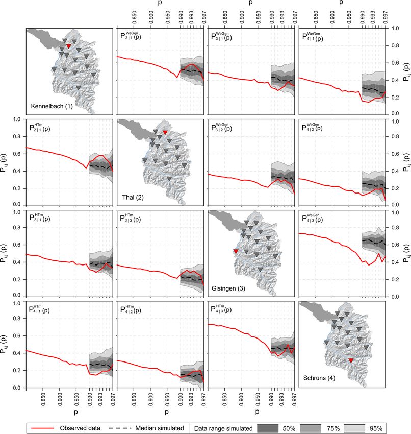
1690                                                  B. Winter et al.: Event generation for probabilistic flood risk modelling

often deployed (e.g. Lamb et al., 2010; Falter et al., 2015;        ferent in their nature. This leads to the key question of the
Schneeberger et al., 2019).                                         present study: does it matter which approach is chosen in
   In a traditional approach, the hydrological load is esti-        the context of flood risk modelling, and what are the advan-
mated by means of extreme-value statistics using river gauge        tages and disadvantages of the two? We answer this question
data and transformed into corresponding inundated areas by          by comparing the set of heterogeneous flood events from the
hydrodynamic models (Teng et al., 2017). The monetary               HT-model with the one resulting from a weather generator
damage can then be assessed in combination with suscepti-           and subsequent rainfall–runoff modelling. Both methods are
bility functions which describe the relationship between one        embedded in a probabilistic flood risk model used to estimate
or more flood hazard characteristics (e.g. inundation depth         the effect of chosen methods on flood losses. To the best of
and flow velocity) and damage for the elements at risk (Merz        the authors’ knowledge, there is no study to date in which
et al., 2010). This approach implies two strong assumptions.        the two approaches are directly compared. Additionally, the
First, the return period of flood discharge is assumed to be        flood risk corresponding to homogeneous flood scenarios of
equal to the return period of the resulting damage. Second, a       certain return periods (“traditional” approach) is derived and
uniform return period across the entire study area is consid-       compared to the other two approaches.
ered and resulting damage estimates are accumulated. The               This paper is organised as follows: first, the study area is
first assumption can be relaxed by modelling a continuous           shortly described. In Sect. 2 the flood risk model is intro-
series of synthetic flood events. As a result, a long series of     duced and the two different approaches for heterogeneous
damage values can be generated and used for analysing dam-          event generation are presented in details. Section 3 presents
age frequency distribution (Achleitner et al., 2016). The sec-      the results of the comparison, which are discussed in the
ond assumption of homogeneous flood return periods may be           following section. Finally, conclusions summarise the major
valid for small areas (de Moel et al., 2015). With increasing       findings.
scale, the assumption of a homogeneous return period be-
comes unlikely, as precipitation and flood footprints are inho-
mogeneous in space. This assumption can lead to an overesti-        2   Study area
mation of risk for specific return periods in large river basins
                                                                    The flood risk model is applied in the westernmost province
(Thieken et al., 2015; Vorogushyn et al., 2018; Metin et al.,
                                                                    of Austria, Vorarlberg. The region is characterised by a
2020). To overcome the second limitation, realistic spatially
                                                                    strong altitudinal gradient between the Rhine River valley
heterogeneous events need to be generated across the area of
                                                                    ( ≈ 400 m a.s.l.) and the high mountain ranges of the Alps
interest which fully represent the spatial variability of flood-
                                                                    (> 3000 m a.s.l.). As a result of the high relief energy, the
ing (Schneeberger et al., 2019).
                                                                    rivers are characterised by a fast hydrological response with
   Generation of spatially heterogeneous flood events in
                                                                    short concentration times. The mountainous landscape of in
terms of precipitation fields or discharges is of current sci-
                                                                    total 2600 km2 is dominated by forest, meadows and pastures
entific interest (Keef et al., 2013; Falter et al., 2015; Falter,
                                                                    with only small percentage of settlement area (Sauter et al.,
2016; de Moel et al., 2015; Speight et al., 2017; Diederen
                                                                    2019). Due to steep topography, asset values are concentrated
et al., 2019; Diederen and Liu, 2019; Schneeberger et al.,
                                                                    in the lowlands of larger valley floors, especially alongside
2019). There are different approaches to generating large
                                                                    the Rhine and Ill rivers. Vorarlberg is characterised by one of
event series of heterogeneous flood events. One possibil-
                                                                    the highest precipitation amounts in Austria, conditioned by
ity is the application of multi-variate statistical methods to
                                                                    predominantly westerly flows and strong orographic effects
discharge series, such as copula models (Jongman et al.,
                                                                    (BMLFUW, 2007). During the last decades, the province
2014; Serinaldi and Kilsby, 2017; Brunner et al., 2019) or
                                                                    was affected by several severe flood events in 1999, 2002,
the semi-parametric conditional model proposed by Heffer-
                                                                    2005 and 2013. The most devastating recent flood event in
nan and Tawn (2004) (hereinafter referred to as “HT-model”
                                                                    August 2005 caused about EUR 180 million direct tangible
or “HTm”). These models consider the pairwise dependence
                                                                    losses for the private and public sector, including infrastruc-
of peak discharges at multiple locations and generate syn-
                                                                    ture (Habersack and Krapesch, 2006). Figure 1 provides an
thetic series of multiple dependent flow peaks. The second
                                                                    overview of the study area, including the river network, set-
possibility is based on the generation of spatially distributed
                                                                    tlement areas and locations of river gauging stations as well
meteorological fields by a weather generator, either station-
                                                                    as meteorological stations.
based with subsequent interpolation (Falter et al., 2016; Fal-
ter, 2016; Breinl et al., 2017; Evin et al., 2018; Raynaud
et al., 2019) or raster-based (Buishand and Brandsma, 2001;         3   Methods and data
Peleg et al., 2017). Synthetic meteorological fields are sub-
sequently used to drive hydrological simulations to generate        The probabilistic flood risk model (PRAMo) used in the pre-
streamflow values across the study area.                            sented work consists of three different modules: the haz-
   The two presented approaches estimate the hydrological           ard module comprising the generation of long time series of
load in the river network at multiple locations but are dif-        flood events; the vulnerability module used to evaluate pos-

Nat. Hazards Earth Syst. Sci., 20, 1689–1703, 2020                                 https://doi.org/10.5194/nhess-20-1689-2020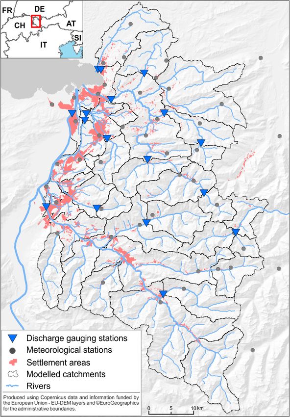
B. Winter et al.: Event generation for probabilistic flood risk modelling                                                    1691

                                                                    able. Stations without hourly information were interpolated
                                                                    by an inverse distance-weighting (IDW) scheme (for details
                                                                    see Winter et al., 2019).

                                                                    3.1   Hazard module I: HT-model

                                                                    The hazard module generates time series of spatially dis-
                                                                    tributed synthetic flood events. In the first approach, we ap-
                                                                    ply the conditional extreme-value model (HT-model) pro-
                                                                    posed by Heffernan and Tawn (2004) to peak flows. In this
                                                                    approach, flood events are understood as a set of spatially
                                                                    consistent peak discharges at multiple locations of stream
                                                                    gauges. Spatial consistency is ensured by considering the
                                                                    correlation structure of peak flows from the past observation
                                                                    period. Discharge time series at 17 gauges across the study
                                                                    area are used to parameterise the HT-model. In the first step,
                                                                    the observed data are standardised by a marginal model to a
                                                                    Laplace distribution. In the second step, the dependency be-
                                                                    tween the stations is modelled for the case of peak flow at one
                                                                    station being above a certain threshold. According to Lamb
                                                                    et al. (2010), the HT-model can be interpreted as a multi-site
                                                                    peak-over-threshold approach. Due to strong seasonality of
                                                                    streamflow in Vorarlberg, the HT-model is separately param-
                                                                    eterised for winter and summer periods (Schneeberger and
                                                                    Steinberger, 2018).
                                                                       For the set of synthetic flood peaks at each of the 17 gauge
                                                                    locations we estimate the return period based on the gener-
                                                                    alised extreme value (GEV). A flood event is characterised
                                                                    by exceedance of a certain streamflow at a single location or
Figure 1. Study area and the location of meteorological and river   multiple locations with a defined time period. As a thresh-
gauging stations.                                                   old for defining a widespread flood event, a return period
                                                                    of 30 years was selected in the present study. The output
                                                                    of the HT-model in terms of synthetic flood peaks is avail-
sible adverse consequences of flood events with a certain ex-       able at the locations of gauging stations. Hence, for the river
ceedance probability; and the risk assessment module, which         segments without observations, the flows and their respec-
combines the results of the hazard and vulnerability mod-           tive return periods need to be estimated. We apply the top-
ules to estimate the loss per event and resulting risk (Schnee-     kriging approach (Skøien et al., 2006) for the spatial inter-
berger et al., 2019). The output of the flood risk model con-       polation of model results to the entire river network. This
sists of expected annual damage and exceedance probabil-            method takes into account the nested structure of river catch-
ity curves of damage. PRAMo was previously driven by                ments, which makes the results more robust compared to tra-
the synthetic flood event series of coherent peak discharges        ditional regional regression-based approaches (Laaha et al.,
generated by the HT-model (Schneeberger and Steinberger,            2014; Archfield et al., 2013). A more detailed description of
2018). A second event generation approach based on a multi-         the HT-model is provided in Schneeberger and Steinberger
site, multi-variate weather generator and continuous rainfall–      (2018) and Schneeberger et al. (2019).
runoff modelling was recently introduced by Winter et al.
(2019) and is used for comparison with the HT-model-based           3.2   Hazard module II: WeGen
approach and the assumption of homogeneous return peri-
ods. Figure 2 provides an overview of the modules and the           The second approach is based on a stochastic weather gen-
simulation steps, which are described in more details in the        erator used to drive a hydrological model. Long-term daily
following.                                                          precipitation and temperature series are generated, with a
   In this study, data of 17 gauging stations (1971–2013) are       multi-site, multi-variate weather generator based on the auto-
applied for the HT approach. The continuous simulation of           regressive model (Hundecha et al., 2009). Daily precipitation
the WeGen approach is based on daily time series from 1971          amounts are generated from mixed gamma and generalised
to 2013 for 45 meteorological stations (cf. Fig. 1). At hourly      Pareto distributions fitted to individual weather stations. The
time steps data for only 23 sites starting from 2001 are avail-     mixed distribution is shown to better capture extreme pre-

https://doi.org/10.5194/nhess-20-1689-2020                                 Nat. Hazards Earth Syst. Sci., 20, 1689–1703, 2020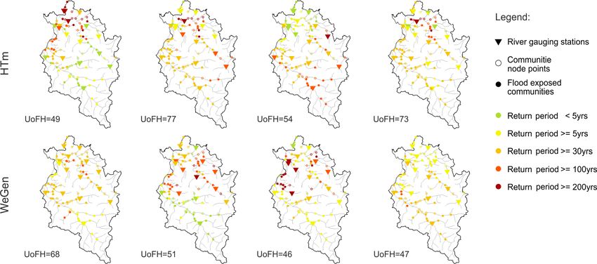
1692                                                  B. Winter et al.: Event generation for probabilistic flood risk modelling

Figure 2. Flowchart of the PRAMo flood risk model including two different approaches for flood event generation.

cipitation while robustly modelling the bulk of precipitation         the variability between the disaggregated days and reduces
amounts (Vrac and Naveau, 2007). With respect to seasonal             the maximum search distance on a temporal scale, especially
patterns, the fitting is applied on a monthly basis. Occur-           for days at the beginning and end of a month.
rence and amount of precipitation are modelled considering               Following the generation of meteorological data at the lo-
the autocorrelation and inter-site correlation structure. The         cations of the weather stations, a spatial interpolation to con-
mean temperature is then modelled conditioned to the simu-            tinuous meteorological fields is necessary for the application
lated precipitation (Hundecha and Merz, 2012). As the study           of the rainfall–runoff model. Complex methods for spatial
area is characterised by mostly alpine topography with short          interpolation can be applied (e.g. Goovaerts, 2000; Plouffe
catchment response times, the hydrological model needs to             et al., 2015); however, for the long-term simulation a compu-
be driven by meteorological input at sub-daily resolution to          tationally efficient approach is needed. The interpolation was
estimate realistic peak flows (e.g. Dastorani et al., 2013). A        carried out by a inverse distance-weighting scheme including
non-parametric k-nearest-neighbour algorithm based on the             a stepwise lapse rate to account for the complex topography
method of fragments is applied to disaggregate the gener-             (Bavay and Egger, 2014).
ated daily values to hourly time steps (Winter et al., 2019).            Finally, the semi-distributed conceptual rainfall–runoff
For a day to disaggregate, the generated daily values of tem-         model HQsim is applied to simulate streamflow across all
perature and precipitation from the weather generator are             catchments of the study area (Kleindienst, 1996). HQsim is
compared against observed daily data at all stations. Subse-          forced by precipitation and temperature data and has previ-
quently, k-nearest neighbours in terms of lowest Euclidean            ously been used in various studies in alpine catchment areas
distances between generated and observed daily values are             (e.g. Senfter et al., 2009; Achleitner et al., 2012; Dobler and
selected. Next, one matching day is randomly sampled from             Pappenberger, 2013; Bellinger, 2015; Winter et al., 2019). A
the selected neighbours, and the corresponding relative tem-          simulated annealing algorithm is used for the model calibra-
poral patterns from the match day are transferred to the input        tion against observed discharge data at the gauging stations
day (method of fragments). In contrast to the previous study          (Andrieu et al., 2003). From a long synthetic discharge se-
(Winter et al., 2019), a centred moving window of 30 d is ap-         ries, relevant flood events are identified and extracted. For
plied instead of the identical months in order to restrict the        this, a flood frequency analysis at all points of interest based
search of possible matching days. The modification increases          on fitting the GEV distribution using the L moments is car-

Nat. Hazards Earth Syst. Sci., 20, 1689–1703, 2020                                    https://doi.org/10.5194/nhess-20-1689-2020
B. Winter et al.: Event generation for probabilistic flood risk modelling                                                   1693

ried out. Analogously to the HT-model approach, a threshold         solute building values indexed to 2013 according to the con-
of a 30-year return period, at least at one site across the study   struction price index (Statistik Austria, 2019) are derived by
area is applied to define relevant flood events. A more de-         calculating mean cubature values from local insurance data
tailed description of the modelling chain, including the dis-       and transferred to the entire building stock of the study area
aggregation procedure, is given in Winter et al. (2019).            (Huttenlau et al., 2015). Since derived values are based on
                                                                    insurance data, they are consequently defined as replacement
3.3   Vulnerability module                                          values.

While the hazard module computes the hydrological load,             3.4   Risk assessment module
the vulnerability module assesses the possible negative con-
sequences in terms of exposed objects and monetary dam-             The risk assessment module brings together the results of the
age. The module is based on the widely used approach of             hazard and vulnerability modules to generate a time series
combining the exposure and susceptibility of elements at            of losses and calculates the resulting risk curve for the area
risk in the inundated areas (Koivumäki et al., 2010; Merz           of interest (Schneeberger et al., 2019). In order to combine
et al., 2010; Huttenlau and Stötter, 2011; Meyer et al., 2013;      the results, each spatial unit (community) is represented by
Cammerer et al., 2013; de Moel et al., 2015; Falter, 2016;          a defined model node point in the river network. For each
Wagenaar et al., 2016). The module calculates losses for            generated heterogeneous flood scenario, the recurrence in-
each community in the study area for a number of prede-             tervals are derived for all model node points (hazard mod-
fined return periods (or probabilities) (i.e. RP = 30, 50, 100,     ule) and combined with the respective loss–probability rela-
200 and 300 years). The results of the vulnerability module         tion to compute losses (vulnerability module). By integrating
are loss–probability relations for each community, describ-         the losses at all model node points, i.e. for each community,
ing the expected damage for the corresponding return peri-          the total loss for every generated event can be calculated. By
ods. To derive a continuous relation, a linear interpolation        evaluating the overall modelled time series of events, a con-
between available data points (RP damage) is applied. The           tinuous time series of damage is generated. Finally, the time
loss–probability relations are used as input in the risk assess-    series of damage can be statistically analysed to derive the
ment module and combined with the simulated return periods          expected annual damage (EAD) and to construct risk curves
(hazard module) at each community to derive risk curves.            (Schneeberger et al., 2019). More detailed information about
   At the scale of a community (on average 28 km2 ), a ho-          the vulnerability and risk assessment module, including a
mogeneous return period of hydrological load is assumed             schematic overview of the module interaction, is provided
and associated with the total community loss. For the loss          in Schneeberger et al. (2019).
calculation we use “official” inundation maps. The inunda-
                                                                    3.5   Assessment of spatial coherence of generated events
tion maps are based on 1-D hydrodynamic modelling in ru-
ral areas and 2-D modelling in urban areas (IAWG, 2010).            A core element of the probabilistic flood risk model is the
The boundary conditions for the hydrodynamic simulation             generation of plausible, spatially heterogeneous flood events.
are taken from the Austrian flood risk zoning project HORA          To investigate the spatial coherence of synthetic events gen-
(Merz et al., 2008).                                                erated by two different approaches, two spatial dependence
   The estimation of monetary damage for the elements at            measures proposed by Keef et al. (2009) are applied. The first
risk is based on the relative damage functions combined with        measure Pi,j (p) describes the probability that a dependent
the total asset values. A damage function describes the rela-       site i exceeds a certain threshold, given that a conditional
tive loss of value as a function of water depth (Merz et al.,       site j is exceeding a threshold qp (Qj ) as well:
2010). If available, additional damage influencing parame-
ters, such as flow velocity or contamination, can be con-           Pi,j (p) = Pr Qi > qp (Qi ) |Qj > qp Qj ,                  (1)
sidered for damage assessment (Merz et al., 2013). In ac-
cordance with Schneeberger et al. (2019), the one paramet-          where (p) is the level of extremeness (quantile) and Qi and
ric damage model of Borter (1999) is applied in the present         Qj are the dependent and conditioned runoff series, respec-
study. The damage model was derived for Switzerland, which          tively. The calculation of the thresholds is based on a 3 d
is a direct neighbour to the Austrian province Vorarlberg with      block maximum, which was found to be appropriate in this
a similar topography and building structure. More precise           region (Schneeberger and Steinberger, 2018). The second
site-specific damage functions are not available for the study      spatial dependence measure Nj (p) is an overall summary
region.                                                             metric and describes the average probability of all dependent
   The damage estimation is conducted on a single-object ba-        sites i to be high, given that the conditional site j is high,
sis for residential buildings only. To derive the flood losses,     defined as
the available inundation maps are combined with the as-                        P
                                                                                  Pr Qi > qp (Qi ) |Qj > qp Qj

set datasets and damage function. Subsequently, the object-                    i6=j
based loss data are aggregated for each community. The ab-          Nj (p) =                                        .          (2)
                                                                                              n−1

https://doi.org/10.5194/nhess-20-1689-2020                                 Nat. Hazards Earth Syst. Sci., 20, 1689–1703, 2020
1694 B. Winter et al.: Event generation for probabilistic flood risk modelling
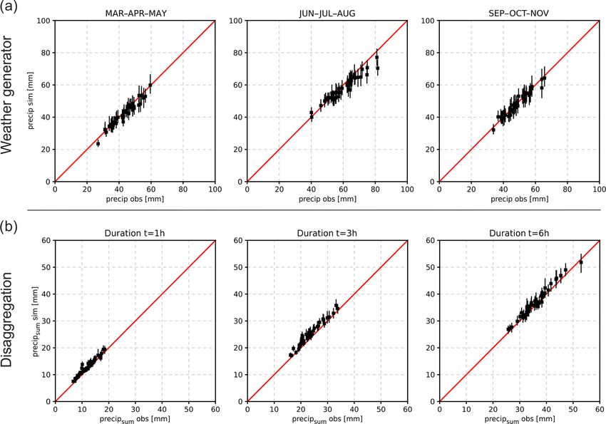
Figure 3. Validation results of the weather generator and the revised disaggregation procedure for all stations (n = 45). The bars represent
the median and the 5–95 % quantile range of 100 realisations for the weather generator and disaggregation. (a) Weather generator: 99 %
quantile of daily precipitation for generated data compared with observed data for spring, summer and autumn. (b) Disaggregation: 99.9 %
quantile of 13 years of disaggregated data is compared to observed data, for the precipitation sum of 1, 3 and 6 h duration.
In the case of the WeGen approach the dependence matri- months separately, including maximum and minimum simu-
ces were computed for the peak discharges at the gauging lated daily temperatures, are provided by Winter et al. (2019).
station locations resulting from the combined simulations of To validate the disaggregation procedure, the hourly data are
the weather generator and rainfall–runoff model. first aggregated to daily data and subsequently disaggregated
back to hourly time steps. For the comparison of disaggre-
gated precipitation, 99, 99.9 and 99.95 % quantiles are calcu-
4 Results lated and compared to the observed values. The results for the
99.9 % quantile show a good agreement between observed
4.1 Simulation results of the continuous modelling and simulated precipitation intensities for the three analysed
approach (WeGen) rainfall durations: 1, 3 and 6 h (Fig. 3b). Results for the 99
and 99.95 % quantile are shown in Winter et al. (2019).
To assess the performance of the continuous modelling ap- The rainfall–runoff model is calibrated (2001–2007) and
proach, extreme precipitation of simulated data is compared validated (2008–2013) in a classical split-sample approach
to observed station data (daily: 1971–2013; hourly: 2001– (Klemeš, 1986) for all catchments of the study area against
2013) for the weather generator and disaggregation proce- observed river gauging data. On average, a Nash–Sutcliffe
dure. The median and the uncertainty range represented by efficiency (NSE; Nash and Sutcliffe, 1970) of 0.68 and 0.67
the 5 and 95 % quantiles of 100 model realisations are com- and a Kling–Gupta efficiency (KGE; Kling et al., 2012)
pared to the observed data. Figure 3a shows the results for of 0.75 and 0.74 are achieved for the calibration and vali-
the 99 % quantile of daily precipitation (wet days) for all dation periods, respectively. Detailed results for the individ-
45 station and spring (March–April–May), summer (June– ual catchments, including a comparison of design flood es-
July–August) and autumn (September–October–November). timates with a flood frequency analysis and a design storm
In general, the characteristics of the observed daily precipi- approach, are given in Winter et al. (2019).
tation are well reproduced by the weather generator. A few
stations, however, show a slight underestimation in sum-
mer (mainly June and August). The validation results for all
Nat. Hazards Earth Syst. Sci., 20, 1689–1703, 2020 https://doi.org/10.5194/nhess-20-1689-2020B. Winter et al.: Event generation for probabilistic flood risk modelling 1695
Figure 4. Comparison of observed (42 years) and simulated conditioned exceedance probability Pi,j (p). The range of the simulated results
is based on 42 years of simulation with 100 realisations. The plots in the lower triangle correspond to the HT model, whereas those in the
upper triangle show the WeGen results.
4.2 Spatial patterns of generated flood events the maps in the principal diagonal. The gauges Kennelbach
and Gisingen are the two largest catchments of the study
For the analysis of spatial coherence, 100 simulations us- area (about 80 % of the total area). The examples Schruns
ing each of the two event generation approaches (HT-model and Thal are subcatchments of Gisingen and Kennelbach,
and WeGen) were carried out. Each simulation comprised respectively, and thus represent two strongly related gauge
42 years of data corresponding to the length of the observed pairs. The measure is calculated for discharge values with
discharge series. Figure 4 illustrates exemplary results for exceedance probability between p = 0.99 and p = 0.997,
four gauging stations and both methods. Each plot shows the above which the data are too few (n < 15) to calculate a
dependence measure between the two stations depicted on meaningful Pi,j value. Based on the empirical distribution
https://doi.org/10.5194/nhess-20-1689-2020 Nat. Hazards Earth Syst. Sci., 20, 1689–1703, 20201696 B. Winter et al.: Event generation for probabilistic flood risk modelling
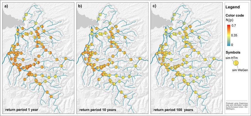
Figure 5. Spatial dependence measure Nj (p) for the community node points at the river network and three different return periods. The
results show the median for the HT-model and WeGen approach based on 30 realisations of 1000 years of simulation.
function of the 3 d block maxima series, a p value of 0.99 are visible. The node points downstream are characterised by
refers to a return period of approximately 1 year, and a a higher dependence. For a high return period of 100 years
p value of 0.997 refers to a return period of roughly 3 years. (Fig. 5c), the simulated spatial dependence is higher for the
In general, the spatial dependence declines with the level HT-model than for the WeGen results in contrast to the find-
of extremeness. For more extreme runoff situations, the de- ings for the lower return periods. The results are regionally
pendence structure is less stable and prone to a large vari- different. Whereas the dependence measure is higher for the
ability. The HT-model results in the lower triangle repro- HT-model in the western part of the study area, the north-
duce the observed spatial patterns between the stations well. eastern catchments show a higher degree of dependence for
The observed measure is in ≈ 90 % of the cases inside the WeGen approach.
the simulated data range (2.5–97.5 % quantile). The results
of the WeGen approach follow the general observed pat- 4.3 Comparison of risk curves
terns of lower dependence (e.g. Pi,j (p) ≈ 0.2 for Thal (2)
vs. Schruns (4)) and higher dependence (e.g. Pi,j (p) ≈ 0.5
for Kennelbach (1) vs. Thal (2)). However, the results are bi- To compare the effect of the two approaches of synthetic
ased towards a higher dependence, such that only half of the event generation on the overall estimated loss, flood risk
results correspond well to the observed data. curves are calculated. Confidence intervals are derived based
To analyse the dependence structure of high flows across on 30 realisations of 1000-year simulations. Furthermore,
the study area, the measure Nj (p) is calculated for all node the risk curve based on the assumption of homogeneous re-
points corresponding to different communities. The measure turn period floods across all catchments is derived based
is calculated for p values corresponding to the 1-, 10- and on five inundation maps corresponding to the return peri-
100-year return period. As the simulation of the two ap- ods between 30 and 300 years. The two synthetic event gen-
proaches is not limited to the length of the observed data, erators result in a comparable range of overall estimated
the results are based on the median of 30 realisations of flood risk (see Fig. 6). The WeGen approach systemati-
1000 years of HT-model and WeGen simulations (Fig. 5). cally overestimates the risk computed by the HT-model.
The length is chosen to be far above the highest return pe- The relative difference between the estimated median values
riod of available homogeneous inundation data (RP300), and ((WeGen−HTm) / WeGen) is approximately 17.5 %. The un-
the number of 30 realisations is dictated by the computa- certainty increases with increasing return period of damage
tional limitations of the continuous simulation at an hourly alongside the extrapolation of the input time series. On aver-
time step. Both approaches (see Fig. 5a–c) show a decline of age 172 damage events are generated per 1000 years of simu-
spatial dependence towards higher return periods. The gen- lation in the WeGen approach, compared to about 167 for the
eral patterns of lower spatial dependence in the southern part HT-model. Both approaches show a significantly lower dam-
of the study area and of the individual northern catchments age in comparison to the assumption of homogeneous sce-
narios for specific return periods. The estimated damage of
Nat. Hazards Earth Syst. Sci., 20, 1689–1703, 2020 https://doi.org/10.5194/nhess-20-1689-2020B. Winter et al.: Event generation for probabilistic flood risk modelling 1697
ing stations. The HT-model makes use of the observed river
gauging data and models their dependence structure directly.
In contrast, the WeGen approach models the dependence
structure only indirectly based on the meteorological input
data.
The overall river network and especially small ungauged
tributaries do however rely on the top-kriging interpolation in
the case of the HT-model approach and are not able to react
independently to the larger river system. This explains the
higher dependence structure on the community node points,
while at the river gauges the results do correspond well to the
observed values. Nevertheless, in both cases the capability to
capture spatial effects of a certain spatial scale in the end
Figure 6. Risk curves for WeGen and HT-model approach in com- depends on the density of the measuring network and its data
parison to the results of a homogeneous scenario. The median quality.
and quantile confidence intervals are based on 30 realisations of The WeGen approach seems to overestimate the overall
1000 years of simulation. Monetary values are normalised to the spatial dependence in the study area in comparison to the
year 2013. observed values. This was also found in a previous study,
comparing a different set of gauging stations (Winter et al.,
2019). One possible reason could be that the spatial interpo-
a homogeneous 100-year flood scenario is ≈ 50 % above the lation of the meteorological data by the rather simple IDW
HT-model results and still 40 % above the WeGen approach. approach, without consideration of shading or other effects,
The sets of generated heterogeneous flood events reflect a and the rather short length of hourly input data for the disag-
large variability of plausible spatial patterns. Hence the esti- gregation procedure might affect the spatial patterns towards
mated flood risk is the result of a combination of these pat- a stronger dependence. More importantly, the WeGen model
terns. Figure 7 shows multiple examples of generated flood itself seems to overestimate the dependence between stations
events corresponding to an estimated damage of EUR 100 ± particularly for higher return period thresholds. This is in line
1 million for both model approaches. The general severity in with the results of the recent evaluation of the weather gener-
terms of flood hazard (without consideration of flood risk) ator (Ullrich et al., 2019), which suggest an overestimation of
is given by the unit of flood hazard (UoFH). The measure correlation of extreme precipitation between individual sta-
UoFH is a simple proxy of hazard severity defined as the total tions leading to an overestimation of areal rainfall. The corre-
number of sites at which the threshold of 30 years return pe- lation structure of the weather generator is fitted on a monthly
riod is exceeded (Schneeberger et al., 2019). Even though the basis, independently of the rainfall intensities, and thus does
selected severity of displayed flood event is rather high, some mix low-intensity, large-scale rainfalls and small-scale con-
of the generated events are still spatially limited. The event vective events. The simulated stronger spatial dependence in
with the lowest UoFH of 46 corresponds to ≈ 50 % of all certain areas with high damage potential also contributes to
sites exceeding the 30-year threshold. The most widespread the higher flood risk estimate by the WeGen approach.
event (UoFH = 77) corresponds to about 90 % of the sites Only one possible combination of weather generator, dis-
exceeding the threshold. This result reflects the spatial dis- aggregation procedure and rainfall–runoff model was applied
tributions of elements at risk with a settlement concentration for the WeGen approach. Thus, by the application of an al-
alongside the larger valley areas in the study area (cf. Fig. 1). ternative weather generator with different assumptions about
Thus, the damage corresponding to an event is largely influ- the spatial dependence or tail distribution, the resulting risk
enced by the region affected. If the overall comparison is con- estimates may change. This counts as well for the applica-
ducted at hazard level only, the impact of widespread flood tion of a different rainfall–runoff model or alternative disag-
events may be overestimated, while the impact of spatially gregation procedure (e.g. Müller-Thomy et al., 2018). Thus,
limited events in densely populated areas is underestimated. the result of a higher risk estimate for the WeGen approach
in comparison to the HT approach can not be generalised to
other model combinations.
5 Discussion The two approaches to synthetic event generation differ
substantially in terms of estimated damage from the one as-
Both approaches, the HT-model and the WeGen approach, suming a uniform return period across the whole study area
simulate complex, spatially heterogeneous patterns of syn- (Fig. 6). The flood losses for individual return periods above
thetic flood events. In the present study, the HT-model out- the 30-year threshold under the homogeneous assumption are
performs the WeGen approach in terms of reproducing the largely overestimated. This result confirms the necessity to
observed dependence patterns of peak flows at the gaug- take heterogeneous spatial patterns into account. An event
https://doi.org/10.5194/nhess-20-1689-2020 Nat. Hazards Earth Syst. Sci., 20, 1689–1703, 20201698 B. Winter et al.: Event generation for probabilistic flood risk modelling
Figure 7. Examples of flood events with an estimated flood damage of EUR 100 ± 1 million flood damage for the HT-model and WeGen
approach. The general severity of flood events is characterised by the unit of flood hazard (UoFH).
where every community in the study area is affected by dis-
charges exceeding the 30-year return period during a single
event is rare. Based on a total of 30 000 years of simulation,
less then 10 % of the communities experience losses simul-
taneously in more than 50 % of events (Fig. 8). It can be ex-
pected that with increasing spatial scale the likelihood that
a large number of communities will experience high return
period discharges and losses in a single event will decrease
(Metin et al., 2020). Therefore, generation of spatially con-
sistent heterogeneous flood events is particularly important
with increasing spatial scale. At the same time, considering
dependence of meteorological and hydrological variables at
multiple locations with increasing scale and an increasing
number of dependent locations becomes more challenging.
A fundamental difference between the two approaches
resides in the way of considering the hydrological pro-
cesses. The HT-model takes a purely statistical approach by Figure 8. Relative number of flood events exceeding a 30-year flood
analysing the dependence of peak discharges above a cer- threshold and corresponding relative number of affected communi-
tain threshold. It does not explicitly consider hydrological ties. The results are based on 30 000 years of simulation.
processes which generate extremes. For instance, the non-
linearity of catchment response is not explicitly taken into
account, but only so far it is imprinted in the previously ob-
parameter identifiability, increase calibration effort and com-
served peaks used for model parameterisation. The combina-
putational burden, and increase input data demand (tempera-
tion of the weather generator and rainfall–runoff modelling
ture, precipitation, radiation, humidity and wind speed).
describes the hydrological processes in a spatially consis-
In general, continuous hydrological modelling generates
tent and time-continuous way. Hence, the effect of soil mois-
full hydrographs at all locations, which allows for direct cou-
ture accumulation and pre-event catchment conditions are
pling with hydraulic models as, for example, applied in Falter
explicitly modelled. By the application of a fully distributed,
et al. (2015) and Falter (2016). The direct coupling of the We-
physically based model, the hydrological process description
Gen approach with a 1-D to 2-D hydrodynamic model would
could even be improved, for example, by solving full en-
also allow consideration of hydrodynamic interactions in the
ergy balance equations for snow melt or evapotranspiration
river network and their possible effect on the risk estimates.
(e.g. Förster et al., 2014, 2018). On the downside, a further
This may, for example, be the reduction of risk downstream
increase in model complexity might compromise the model
due to dike overtopping and failure upstream. In the case of
Nat. Hazards Earth Syst. Sci., 20, 1689–1703, 2020 https://doi.org/10.5194/nhess-20-1689-2020B. Winter et al.: Event generation for probabilistic flood risk modelling 1699
Table 1. Summary of advantages and disadvantages of the WeGen and HT-model approach to generating heterogeneous flood events.
Categories HT-model WeGen
Computational complexity (+) Low processing costs (local processing) (−) Processing intensive (HPC necessary)
(−) Complex data interfaces between
different models
Output (−) Return periods at all sites for modelled (+) Continuous hydrographs at all modelled
events only sites
Hydraulic coupling (−) Event hydrographs need to be deducted (+) Continuous description of hydraulic
to drive a hydraulic model boundary conditions allows unsteady
hydraulic modelling
Processes (−) No information about individual (+) Continuous description of hydrological
hydrological processes system and modelled processes
Hydrological changes (−) No explicit modelling of scenarios (e.g. (+) Scenarios can be modelled explicitly
climate or land-use scenarios) possible (e.g. climate or land-use scenarios)
(+) Runoff trends can be integrated
Transferability (+) Model is well transferable to other study (−) Model chain is transferable; however
areas all components must be set up and
calibrated for new study areas
the HT-model, only peak discharge of events is estimated, not The presented approaches are subject to different uncer-
the entire hydrograph. Hence, these results cannot be used tainties. The confidence intervals presented in Fig. 6 are,
directly as a boundary condition for unsteady hydraulic sim- for example, based on the random processes generating het-
ulations. Assumptions on the shape of a hydrograph would erogeneous flood events of each method (multiple realisa-
be required. tions). However, there are other uncertainties which are not
In addition, the continuous modelling approach is capa- explicitly addressed, for example uncertainties related to the
ble of explicitly modelling scenarios of changing hydrolog- topological kriging of the HT-model results or uncertain-
ical boundary conditions. For instance, changes in the cli- ties related to the hydrological model in the WeGen ap-
mate system can be taken into account in the generation of proach. Some uncertainties pertain to both methods, such as
meteorological fields by conditioning the rainfall and tem- the choice and fitting of the extreme-value distributions. A
perature probability distributions (e.g. Hundecha and Merz, comprehensive assessment by propagating the uncertainties
2012). Also possible changes in land use can be considered of all sub-models throughout the model chain is currently
by parameterising hydrological models accordingly (Rogger precluded by computational constraints particularly relevant
et al., 2017). As the HT-model approach is based on observed for the WeGen approach.
streamflow only, change scenarios may be included in terms A further important point, currently not considered in both
of trends. However, they cannot be modelled explicitly. A approaches, is dike failure scenarios. In the study area, for
continuous simulation approach requires a vast amount of example, no inundation is considered for the Rhine River due
processed data, including multiple data interfaces between to its high protection level. Nonetheless, the probability of a
the different modelling steps and results in high computa- dike failure is non-zero and could have a devastating effect.
tional costs. This is especially true if sub-daily simulations In this sense, the consideration of flood volumes beside peak
are applied that require an additional disaggregation scheme. estimates could be another important extension to describe
In contrast, the purely statistical HT-model shows its merit the severity of flood events (e.g. Dung et al., 2015; Lamb
with its efficient data processing, easily applicable on local et al., 2016).
computers. A further advantage of the HT-model is the trans- A traditional validation of the overall risk model in terms
ferability of the approach. While each of the modelling steps of a comparison of observed to simulated data is hardly pos-
of the continuous approach, from the weather generator to sible as comprehensive databases of loss events are often not
the hydrological models, needs to be implemented, calibrated available (Thieken et al., 2015). In the present study, damage
and validated for every new study area, the HT-model only data based on an insurance portfolio were available for the
needs to be fitted to new discharge time series which is less 2005 event. The data are, however, only a subset of the over-
complex. Different advantages and disadvantages of both ap- all elements at risk, and, due to rather low sublimits (maxi-
proaches are summarised in Table 1. mum insurance payout), the full losses remain unknown. Fi-
nally, without a larger set of loss events it is not possible to
https://doi.org/10.5194/nhess-20-1689-2020 Nat. Hazards Earth Syst. Sci., 20, 1689–1703, 20201700 B. Winter et al.: Event generation for probabilistic flood risk modelling
assign a meaningful return period to the 2005 event to val- Author contributions. Based on the initial ideas of KS and SV, the
idate the risk outcome in a traditional way. Nonetheless, by study was designed in collaboration with all authors. BW prepared
applying and comparing different methods, the plausibility the initial data, implemented and applied the continuous modelling
of the results can be checked (Molinari et al., 2019). Fur- approach and analysed the results. KF programmed the spatial in-
thermore, the uncertainties related to the choice of methods terpolation scheme for the meteorological data and supported the
rainfall–runoff modelling. The risk model and the HT application
for generating heterogeneous flood events seem to be lower
were mainly developed by KS. The manuscript was drafted by BW
in comparison to other aspects of the probabilistic flood risk with support of SV. All authors contributed to the review and final
model, such as the choice of the applied damage functions version of the manuscript.
(Winter et al., 2018).
Competing interests. The authors declare that they have no conflict
6 Conclusions
of interest.
The question of whether the choice of method for generating
heterogeneous flood events for flood risk modelling matters
Acknowledgements. We thank all the institutions that pro-
can be answered in different ways. Both approaches, the HT-
vided data, the Zentralanstalt für Meteorologie and Geody-
model and continuous WeGen approach, were generally ca- namik (ZAMG), the Deutscher Wetterdienst (DWD), and particu-
pable of modelling spatially plausible flood events across the larly the Hydrographischer Dienst Vorarlberg. The simulations were
study area. By direct comparison to observed spatial patterns, conducted using the Vienna Scientific Cluster (VSC). Finally, we
the HT-model approach performed better than the WeGen ap- want to thank the editor, Margreth Keiler, and the two reviewers
proach in our study area in terms of correctly representing (Martina Kauzlaric and anonymous) for taking their time to criti-
the observed dependence structure. A stronger modelled de- cally evaluate this article and to provide valuable and constructive
pendence of extreme precipitation resulted in high areal rain- feedback.
fall in the WeGen approach and higher overall risk compared
to the HT-model. The median damage from 30 000 years of
simulation is about 17.5 % larger in the WeGen approach Financial support. This work results from the research project
than in the HT-model. The representation of the dependence HiFlow-CMA (KR15AC8K12522) funded by the Austrian Climate
structure for simulation of extremes needs to be further im- and Energy Fund (ACRP 8th call). Furthermore, we would like to
thank the vice-rectorate for research and the faculty of Geo- and
proved for the weather generator. Nevertheless, the choice
Atmospheric Sciences at the University of Innsbruck for providing
of method for generating heterogeneous flood events might
open-access funding.
have a smaller impact than, for example, the choice of the
applied damage functions (Winter et al., 2018).
To conclude, both methods are valid approaches to over- Review statement. This paper was edited by Margreth Keiler and
coming the simplified assumption of uniform return period reviewed by Martina Kauzlaric and one anonymous referee.
across a study area. Accordingly, when designing a flood risk
study, the choice of the approach should consider the specific
advantages and disadvantages of the two methods and data
availability. If computational efficiency and quick transfer- References
ability are in focus, the HT-model approach might be a bet-
ter choice. In contrast, if unsteady hydraulic modelling is re- Achleitner, S., Schöber, J., Rinderer, M., Leonhardt, G., Schöberl,
quired for the targeted application, the continuous modelling F., Kirnbauer, R., and Schönlaub, H.: Analyzing the op-
of generated meteorological fields is more appropriate. erational performance of the hydrological models in an
alpine flood forecasting system, J. Hydrol., 412–413, 90–100,
https://doi.org/10.1016/j.jhydrol.2011.07.047, 2012.
Achleitner, S., Huttenlau, M., Winter, B., Reiss, J., Plörer, M., and
Code and data availability. For Austria, daily meteorological and
Hofer, M.: Temporal development of flood risk considering set-
river gauging data are available at https://ehyd.gv.at (last access:
tlement dynamics and local flood protection measures on catch-
28 May 2020) (BMLRT, 2020). The applied meteorological data
ment scale: An Austrian case study, Int. J. River Basin Manage.,
for the Deutscher Wetterdienst (DWD) stations are freely avail-
14, 273–285, https://doi.org/10.1080/15715124.2016.1167061,
able at https://opendata.dwd.de (last access: 28 May 2020) (DWD,
2016.
2020). Underlying loss data are not publicly available. The Me-
Andrieu, C., Freitas, N., Doucet, A., and Jordan, M.: An Introduc-
teoIO is available at https://models.slf.ch/p/meteoio/ (last accss:
tion to MCMC for Machine Learning, Mach. Learn., 50, 5–43,
28 May 2020) (Bavay and Egger, 2014). The applied weather gener-
https://doi.org/10.1023/A:1020281327116, 2003.
ator and the rainfall–runoff model HQsim are currently not publicly
Archfield, S. A., Pugliese, A., Castellarin, A., Skøien, J. O., and
available.
Kiang, J. E.: Topological and canonical kriging for design flood
prediction in ungauged catchments: An improvement over a
traditional regional regression approach?, Hydrol. Earth Syst.
Nat. Hazards Earth Syst. Sci., 20, 1689–1703, 2020 https://doi.org/10.5194/nhess-20-1689-2020B. Winter et al.: Event generation for probabilistic flood risk modelling 1701 Sci., 17, 1575–1588, https://doi.org/10.5194/hess-17-1575-2013, DWD – Deutscher Wetterdienst: Open Data-Server, available at: 2013. https://opendata.dwd.de/, last access: 28 May 2020. Bavay, M. and Egger, T.: MeteoIO 2.4.2: a preprocessing library European Union: European Union on the assessment and manage- for meteorological data, Geosci. Model Dev., 7, 3135–3151, ment of flood risks: Directive 2007/60/EC of the European Par- https://doi.org/10.5194/gmd-7-3135-2014, 2014. liament and the Council, Official Journal of the European Com- Bellinger, J.: Uncertainty Analysis of a hydrological model within munity, Luxembourg, 2007. the Flood Forecasting of the Tyrolean River Inn, Dissertation, European Union: on the taking-up and pursuit of the business of University of Innsbruck, Innsbruck, 2015. Insurance and Reinsurance (Solvency II): Directive 2009/138/EC BMLFUW (Ed.): Hydrologischer Atlas Österreichs, 3. Lieferung, of the European Parliament and the Council, Official Journal of Wien, 2007. the European Union, Luxembourg, 2009. BMLRT – Bundesministerium für Landwirtschaft, Regionen und Evin, G., Favre, A.-C., and Hingray, B.: Stochastic generation of Tourismus: eHYD, available at: https://ehyd.gv.at/, last access: multi-site daily precipitation focusing on extreme events, Hy- 28 May 2020. drol. Earth Syst. Sci., 22, 655–672, https://doi.org/10.5194/hess- Borter, P.: Risikoanalyse bei gravitativen Naturgefahren: Fall- 22-655-2018, 2018. beispiele und Daten, Naturgefahren, Bern, 1999. Falter, D.: A novel approach for large-scale flood risk assessments: Breinl, K., Strasser, U., Bates, P., and Kienberger, S.: A joint mod- continuous and long-term simulation of the full flood risk chain, elling framework for daily extremes of river discharge and pre- Dissertation, University of Potsdam, Potsdam, 2016. cipitation in urban areas, J. Flood Risk Manage., 10, 97–114, Falter, D., Schröter, K., Dung, N. V., Vorogushyn, S., Kreibich, https://doi.org/10.1111/jfr3.12150, 2017. H., Hundecha, Y., Apel, H., and Merz, B.: Spatially coherent Brunner, M. I., Furrer, R., and Favre, A.-C.: Modeling the spa- flood risk assessment based on long-term continuous simula- tial dependence of floods using the Fisher copula, Hydrol. tion with a coupled model chain, J. Hydrol., 524, 182–193, Earth Syst. Sci., 23, 107–124, https://doi.org/10.5194/hess-23- https://doi.org/10.1016/j.jhydrol.2015.02.021, 2015. 107-2019, 2019. Falter, D., Dung, N. V., Vorogushyn, S., Schröter, K., Hundecha, Buishand, T. A. and Brandsma, T.: Multisite simulation of daily Y., Kreibich, H., Apel, H., Theisselmann, F., and Merz, B.: precipitation and temperature in the Rhine Basin by nearest- Continuous, large-scale simulation model for flood risk as- neighbor resampling, Water Resour. Res., 11, 2761–2776, sessments: proof-of-concept, J. Flood Risk Manage., 9, 3–21, https://doi.org/10.1029/2001WR000291, 2001. https://doi.org/10.1111/jfr3.12105, 2016. Cammerer, H., Thieken, A. H., and Lammel, J.: Adaptabil- Förster, K., Meon, G., Marke, T., and Strasser, U.: Effect of ity and transferability of flood loss functions in residen- meteorological forcing and snow model complexity on hy- tial areas, Nat. Hazards Earth Syst. Sci., 13, 3063–3081, drological simulations in the Sieber catchment (Harz Moun- https://doi.org/10.5194/nhess-13-3063-2013, 2013. tains, Germany), Hydrol. Earth Syst. Sci., 18, 4703–4720, Dastorani, M., Koochi, J., and Darani, H. S.: River instan- https://doi.org/10.5194/hess-18-4703-2014, 2014. taneous peak flow estimation using daily flow data and Förster, K., Garvelmann, J., Meißl, G., and Strasser, machine-learning-based models, J. Hydroinform., 15, 1089– U.: Modelling forest snow processes with a new ver- 1098, https://doi.org/10.2166/hydro.2013.245, 2013. sion of WaSiM, Hydrolog. Sci. J., 63, 1540–1557, de Moel, H., Jongman, B., Kreibich, H., Merz, B., Penning- https://doi.org/10.1080/02626667.2018.1518626, 2018. Rowsell, E., and Ward, P. J.: Flood risk assessments at different Goovaerts, P.: Geostatistical approaches for incorporating elevation spatial scales, Mitig. Adapt. Strat. Global Change, 20, 865–890, into the spatial interpolation of rainfall, J. Hydrol., 228, 113–129, https://doi.org/10.1007/s11027-015-9654-z, 2015. https://doi.org/10.1016/S0022-1694(00)00144-X, 2000. Diederen, D. and Liu, Y.: Dynamic spatio-temporal generation of Habersack, H. and Krapesch, G.: Hochwasser 2005 – Ereignis- large-scale synthetic gridded precipitation: with improved spa- dokumentation: der Bundeswasserbauverwaltung, des Forsttech- tial coherence of extremes, Stoch. Environ. Res. Risk Assess., nischen Dienstes für Wildbach- und Lawinenverbauung und des https://doi.org/10.1007/s00477-019-01724-9, in press, 2019. Hydrographischen Dienstes, BMLFUW, Wien, 2006. Diederen, D., Liu, Y., Gouldby, B., Diermanse, F., and Voro- Heffernan, J. E. and Tawn, J. A.: A conditional approach for mul- gushyn, S.: Stochastic generation of spatially coherent river tivariate extreme values (with discussion), J. Roy. Stat. Soc. B, discharge peaks for continental event-based flood risk as- 66, 497–546, https://doi.org/10.1111/j.1467-9868.2004.02050.x, sessment, Nat. Hazards Earth Syst. Sci., 19, 1041–1053, 2004. https://doi.org/10.5194/nhess-19-1041-2019, 2019. Hoegh-Guldberg, O., Jacob, D., Taylor, M., Bindi, M., Brown, S., Dobler, C. and Pappenberger, F.: Global sensitivity analyses for a Camilloni, I., Diedhiou, A., Djalante, R., Ebi, K. L., Engelbrecht, complex hydrological model applied in an Alpine watershed, Hy- F., Guiot, J., Hijioka, Y., Mehrotra, S., Payne, A., Seneviratne, drol. Process., 27, 3922–3940, https://doi.org/10.1002/hyp.9520, S. I., Thomas, A., Warren, R., and Zhou, G.: Impacts of 1.5 ◦ C 2013. Global Warming on Natural and Human Systems, in: Global Downton, M. W. and Pilke, R. A.: How Accurate are Disaster Loss Warming of 1.5 ◦ C. An IPCC Special Report on the impacts Data? The Case of U.S. Flood Damage, Nat. Hazards, 35, 211– of global warming of 1.5 ◦ C above pre-industrial levels and re- 228, https://doi.org/10.1007/s11069-004-4808-4, 2005. lated global greenhouse gas emission pathways, in the context of Dung, N. V., Merz, B., Bárdossy, A., and Apel, H.: Handling uncer- strengthening the global response to the threat of climate change, tainty in bivariate quantile estimation – An application to flood sustainable development, and efforts to eradicate poverty, edited hazard analysis in the Mekong Delta, J. Hydrol., 527, 704–717, by: Masson-Delmotte, V., Zhai, P., Pörtner, H.-O., Roberts, D., https://doi.org/10.1016/j.jhydrol.2015.05.033, 2015. Skea, J., Shukla, P. R., Pirani, A., Moufouma-Okia, W., Péan, https://doi.org/10.5194/nhess-20-1689-2020 Nat. Hazards Earth Syst. Sci., 20, 1689–1703, 2020
You can also read