NEPAL AMBIENT MONITORING AND SOURCE TESTING EXPERIMENT (NAMASTE): EMISSIONS OF PARTICULATE MATTER AND SULFUR DIOXIDE FROM VEHICLES AND BRICK KILNS ...
←
→
Page content transcription
If your browser does not render page correctly, please read the page content below
Atmos. Chem. Phys., 19, 8209–8228, 2019
https://doi.org/10.5194/acp-19-8209-2019
© Author(s) 2019. This work is distributed under
the Creative Commons Attribution 4.0 License.

Nepal Ambient Monitoring and Source Testing Experiment
(NAMaSTE): emissions of particulate matter and sulfur dioxide
from vehicles and brick kilns and their impacts on air quality in the
Kathmandu Valley, Nepal
Min Zhong1,a , Eri Saikawa1,2 , Alexander Avramov1 , Chen Chen1 , Boya Sun1,c , Wenlu Ye2 , William C. Keene3 ,
Robert J. Yokelson4 , Thilina Jayarathne5,b , Elizabeth A. Stone5 , Maheswar Rupakheti6 , and Arnico K. Panday7
1 Department    of Environmental Sciences, Emory University, Atlanta, GA, USA
2 Rollins  School of Public Health, Emory University, Atlanta, GA, USA
3 Department of Environmental Sciences, University of Virginia, Charlottesville, VA, USA
4 Department of Chemistry, University of Montana, Missoula, MT, USA
5 Department of Chemistry, University of Iowa, Iowa City, IA, USA
6 Institute for Advanced Sustainability Studies, Potsdam, Germany
7 International Centre for Integrated Mountain Development (ICIMOD), Khumaltar, Lalitpur, Nepal
a now at: Environmental Analysis and Outcomes Division, Minnesota Pollution Control Agency, MN, USA
b now at: Department of Chemistry, Purdue University, West Lafayette, IN, USA
c now at: Rubicon Global, Atlanta, GA, USA

Correspondence: Eri Saikawa (eri.saikawa@emory.edu)

Received: 19 June 2018 – Discussion started: 15 August 2018
Revised: 12 April 2019 – Accepted: 5 June 2019 – Published: 24 June 2019

Abstract. Air pollution is one of the most pressing environ-     SO2 emissions considered in HTAP_v2.2. Next, we simu-
mental issues in the Kathmandu Valley, where the capital city    lated air quality using the Weather Research and Forecast-
of Nepal is located. We estimated emissions from two of the      ing model coupled with Chemistry (WRF-Chem) for April
major source types in the valley (vehicles and brick kilns)      2015 based on three different emissions scenarios: HTAP
and analyzed the corresponding impacts on regional air qual-     only, HTAP with updated vehicle emissions, and HTAP with
ity. First, we estimated the on-road vehicle emissions in the    both updated vehicle and brick kilns emissions. Compar-
valley using the International Vehicle Emissions (IVE) model     isons between simulated results and observations indicate
with local emissions factors and the latest available data for   that the model underestimates observed surface elemental
vehicle registration. We also identified the locations of the    carbon (EC) and SO2 concentrations under all emissions sce-
brick kilns in the Kathmandu Valley and developed an emis-       narios. However, our updated estimates of vehicle emissions
sions inventory for these kilns using emissions factors mea-     significantly reduced model bias for EC, while updated emis-
sured during the Nepal Ambient Monitoring and Source Test-       sions from brick kilns improved model performance in simu-
ing Experiment (NAMaSTE) field campaign in April 2015.           lating SO2 . These results highlight the importance of improv-
Our results indicate that the commonly used global emis-         ing local emissions estimates for air quality modeling. We
sions inventory, the Hemispheric Transport of Air Pollu-         further find that model overestimation of surface wind leads
tion (HTAP_v2.2), underestimates particulate matter emis-        to underestimated air pollutant concentrations in the Kath-
sions from vehicles in the Kathmandu Valley by a factor          mandu Valley. Future work should focus on improving lo-
greater than 100. HTAP_v2.2 does not include the brick sec-      cal emissions estimates for other major and underrepresented
tor and we found that our sulfur dioxide (SO2 ) emissions es-    sources (e.g., crop residue burning and garbage burning) with
timates from brick kilns are comparable to 70 % of the total     a high spatial resolution, as well as the model’s boundary-

Published by Copernicus Publications on behalf of the European Geosciences Union.
8210                                                               M. Zhong et al.: Vehicle and brick kiln emissions in Nepal

layer representation, to capture strong spatial gradients of air    chimney Bull’s trench kiln (FCBTK) technology and its vari-
pollutant concentrations.                                           ations such as zigzag kilns. In the Kathmandu Valley, brick
                                                                    kilns typically operate for 6 months a year, generally from
                                                                    December to May. The main fuels burned in brick kilns are
                                                                    biomass and high-sulfur coal (Joshi and Dudani, 2008), both
1   Introduction                                                    of which emit SO2 and PM but in differing amounts. Burn-
                                                                    ing biomass emits relatively greater amounts of PM, whereas
Air pollution is one of the most pressing environmental is-         coal combustion emits relatively greater amounts of SO2
sues in South Asia. According to the 2016 Environmental             (Stockwell et al., 2016; Jayarathne et al., 2018). Weyant et al.
Performance Index, air quality in Nepal ranked fourth worst         (2014) estimate the total emissions from the brick industry
in the world (Angel and Alisa, 2016) and Kathmandu, its cap-        in South Asia to be 120 Tg yr−1 carbon dioxide, 2.5 Tg yr−1
ital and largest metropolis, is one of the most polluted cities     CO, 0.19 Tg yr−1 PM2.5 (PM with an aerodynamic diameter
in Asia. Kathmandu lies in a bowl-shaped valley with a floor        less than 2.5 µm), and 0.12 Tg yr−1 EC. Pariyar et al. (2013)
elevation of ∼ 1300 m surrounded by mountains of 2000 to            report that brick kilns contribute more than 60 % of total SO2
2800 m. It is inhabited by approximately 2.5 million people         and PM emissions in the Kathmandu Valley. Using a source
with a steady population growth of 4 % yr−1 (Muzzini and            apportionment method, Kim et al. (2015) found that brick
Aparicio, 2013). The primary sources of air pollution within        kilns contribute 40 % of EC concentrations in the Kathmandu
the valley are uncontrolled emissions from vehicles, brick          Valley in winter. Despite being one of the major sources of
kilns, and biomass and garbage combustion coupled with              air pollution, brick kiln emissions are not included in the
dust originating from both local fugitive emissions and long-       existing gridded inventory estimates. The developers of the
distance transport (Gronskei et al., 1996; Kim et al., 2015;        Regional Emission inventory in ASia version 2 (REAS v2;
Shakya et al., 2010; Stone et al., 2010, 2012). The unique          Kurokawa et al., 2013) discussed that brick kilns are one of
topography coupled with high emissions of pollutants con-           the major sources of EC, but their inventory did not include
tribute to low air quality in the valley.                           emissions from this sector. HTAP_v2.2 uses REAS v2 for
   The rapid growth of the vehicle fleet is of particular con-      Nepal and thus does not include emissions from brick kilns
cern. According to the Department of Transport Management           in their inventory either. Due to the lack of gridded emis-
(DoTM) in Nepal, the total number of registered vehicles in         sions estimates, to date, no studies have explicitly simulated
the Bagmati Zone (most of which operate in the Kathmandu            the impacts of brick kiln emissions on regional air quality.
Valley) increased from 292 697 to 922 831 (12 % yr−1 ), be-            The purpose of this study was to analyze the emissions and
tween 2005 and 2015 (DoTM, 2017). Approximately 80 % of             air quality impacts due to on-road vehicles and brick kilns in
the total registered vehicles are motorcycles, while cars and       the Kathmandu Valley. Mues et al. (2018) reported that an
pickup trucks account for another 13 %. These vehicles emit         emissions database is essential to improve the simulation of
air pollutants, including carbon monoxide (CO), nitrogen ox-        EC using regional chemical transport models in the Kath-
ides (NOx = NO + NO2 ), non-methane volatile organic com-           mandu region. We first estimated on-road traffic emissions
pounds (NMVOCs), particulate matter (PM), elemental car-            using the latest number of registered vehicles and emissions
bon (EC), and organic carbon (OC). Buses were estimated to          factors generated for local conditions. We also created a point
emit more than 90 % of OC, EC, and NOx among all vehi-              source emissions inventory for brick kilns using the newly
cles, while motorcycles were estimated to emit large amounts        measured emissions factors in the Kathmandu Valley. In the
of CO (50 %) and NMVOCs (66 %) by Shrestha et al. (2013).           recent Nepal Ambient Monitoring and Source Testing Ex-
In 2010, the annual emissions of EC and OC from diesel-             periment (NAMaSTE) in April 2015, in situ emissions from
powered vehicles in the Kathmandu Valley were estimated at          several important under-characterized combustion emissions
2117 and 570 t yr−1 , respectively (Shrestha et al., 2013). Rel-    sources were measured, including brick kilns and motorcy-
ative to estimates for the Kathmandu Valley in 2010 based on        cles (Jayarathne et al., 2018; Stockwell et al., 2016). Emis-
the global emissions inventory Hemispheric Transport of Air         sions factors obtained from NAMaSTE were used to create
Pollution (HTAP_v2.2; Janssens-Maenhout et al., 2015), the          the point source emissions inventory of brick kilns. We then
above estimates for vehicle emissions of EC and OC are 80           modified the HTAP_v2.2 estimates with updated emissions
and 20 times higher, respectively, than those estimated for all     from vehicles and brick kilns. Next, we conducted three sim-
sectors combined in HTAP. Considering that Shrestha et al.          ulations using Weather Research and Forecasting model cou-
(2013) did not include emissions from personal cars or trucks       pled with Chemistry (WRF-Chem) to explore the impacts of
in their estimates, vehicle emissions in the Kathmandu Valley       emissions from vehicles and brick kilns on the local air qual-
appear to be significantly underestimated in HTAP_v2.2.             ity. These three simulations differed only in emissions sce-
   More than 100 brick kilns of different types throughout the      narios for vehicles and brick kilns; all other model conditions
Kathmandu Valley produce over 600 million bricks per year           were kept the same.
(Quest Forum Pvt. Ltd, 2017; Gronskei et al., 1996; Weyant
et al., 2014). The majority of these kilns (97 %) use the fixed-

Atmos. Chem. Phys., 19, 8209–8228, 2019                                              www.atmos-chem-phys.net/19/8209/2019/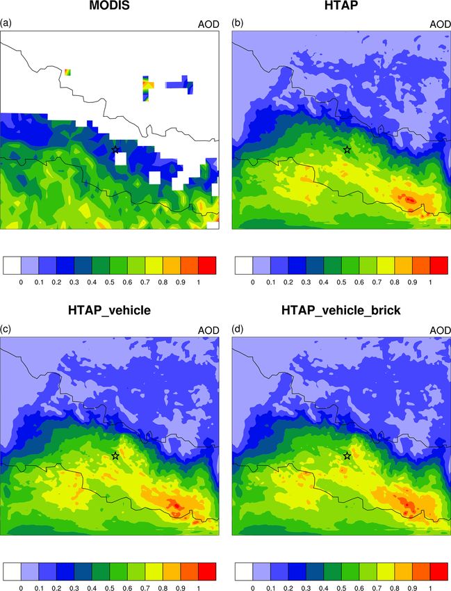
M. Zhong et al.: Vehicle and brick kiln emissions in Nepal                                                                   8211

2     Method                                                          To analyze the impact of emissions from vehicles and
                                                                   brick kilns on air quality in the Kathmandu Valley, we per-
2.1    WRF-Chem model description                                  formed a set of three nested model simulations, referred to as
                                                                   HTAP, HTAP_vehicle, and HTAP_vehicle_brick. The HTAP
We used the regional chemical transport model WRF-Chem             simulation used the original HTAP_v2.2 emissions inventory
version 3.5 in this study. The Regional Atmospheric Chem-          as inputs. The HTAP_vehicle simulation used HTAP_v2.2
istry Mechanism (RACM) (Stockwell et al., 1997) is used for        with updated vehicle emissions (Sect. 2.2.1) as inputs. The
gas-phase reactions. Aerosol chemistry is represented by the       HTAP_vehicle_brick simulation used the HTAP_v2.2 with
Model Aerosol Dynamics for Europe with the Secondary Or-           updated vehicle emissions and the additional brick kiln emis-
ganic Aerosol Model (MADE/SORGAM) (Ackermann et al.,               sions (Sect. 2.2.2) as inputs. The same meteorology and
1998; Schell et al., 2001). MADE/SORGAM predicts the               boundary inputs were used for all three nesting simulations
mass of several particulate-phase species, including sulfate,      as our focus is to understand the impact of emissions on the
ammonium, nitrate, sea salt, dust, EC, OC, and secondary           local air quality. We conducted each simulation for the 2-
organic aerosols in the three aerosol modes (Aitken, accu-         week period of 12–24 April 2015 during which observational
mulation, and coarse). This aerosol model has been widely          data from the NAMaSTE field campaign were available for
used in previous studies (e.g., Gao et al., 2014; Kumar et al.,    comparison (Sect. 2.3). The model was spun up for 5 d pre-
2012; Saikawa et al., 2011; Tuccella et al., 2012; Zhong et al.,   ceding the simulation period, which was sufficient to venti-
2016). Photolysis rates are based on the Fast-J photolysis         late the regional domain.
scheme (Wild et al., 2000). The Rapid Radiative Transfer
Model (RRTM) (Mlawer et al., 1997) accounts for aerosol            2.2     Emissions
radiative feedbacks. Lin et al. (1983) and one and a half lo-
cal Mellor–Yamada–Nakanishi–Niino Level 2.5 (Nakanishi             2.2.1    Emissions scenarios in 2015
and Niino, 2006) schemes are used to parameterize cloud
microphysical and sub-grid processes in the planetary bound-       We used three emissions scenarios (Table 1) to investigate
ary layer (PBL), respectively. The horizontal winds, temper-       the impact of emissions on local air quality in the Kath-
ature, and moisture at all vertical levels are nudged to the       mandu Valley. The first emissions scenario is the same as
large-scale meteorological fields from the National Centers        the original HTAP_v2.2 (Janssens-Maenhout et al., 2015).
for Environmental Prediction (NCEP) Global Forecast Sys-           HTAP is a gridded global emissions inventory combined
tem final gridded analysis datasets.                               with the regional inventories and gap-filled with the Emis-
   The model domain covered large parts of the Himalayas,          sions Database for Global Atmospheric Research (EDGAR
India, Nepal, and southwest China (Fig. 1). The domain in-         v4.3) (Janssens-Maenhout et al., 2013). In Asia, HTAP_v2.2
cluded three levels of one-way nesting with horizontal grid        uses the MIX inventory, a regional emissions inventory in
spacing of 27, 9, and 3 km, each of which was centered             Asia, which is also developed based on the “mosaic” ap-
on the Kathmandu Valley. The topography of the innermost           proach including multiple existing national inventories (Li
model domain is complicated, with the Himalayan range sit-         et al., 2017). The second emissions scenario utilizes the origi-
ting across west to east and separating the Indian subcon-         nal HTAP_v2.2 with updated vehicle emissions (Sect. 2.2.2).
tinent from the Tibetan Plateau. Even when we use 3 km             The third scenario is built on the second scenario and adding
spacing for the nested domain, the model is unable to re-          emissions from brick kilns (Sect. 2.2.3). We used the latest
solve the very steep topographic features but this was the         available HTAP_v2.2 for 2010 as the baseline inventory, as
best we could do with this project, given the resolution of        this is the closest year to 2015 that we have the data for. The
emissions available. There are 31 vertical levels from the sur-    vehicle and brick kiln emissions were developed for the year
face to 50 mbar. The Model for Ozone and Related Chemical          2015.
Tracers (MOZART) global chemical transport model (Em-
mons et al., 2010) was used to provide initial and lateral         2.2.2    Emissions from vehicles
boundary conditions for chemical species in the outermost
domain. We found that the inclusion of dust from MOZART            Emissions from the road transport sector in the Kathmandu
led to overestimated aerosol optical depth (AOD) at Jomsom         Valley were estimated using the International Vehicle Emis-
in Nepal and at Qomolangma (Mt. Everest) station for Atmo-         sions (IVE) model version 2.0 (Davis et al., 2005). The IVE
spheric and Environmental Observation and Research, Chi-           model is specifically designed to calculate emissions from
nese Academy of Sciences (QOMS_CAS) in Tibet, China.               motor vehicles in developing countries for local conditions
Therefore, in our simulations, dust concentrations were cal-       and has been used extensively in several countries world-
culated online, using the Air Force Weather Agency (AFWA)          wide, including Nepal (Shrestha et al., 2013), India (Barth
emissions scheme (Marticorena and Bergametti, 1995) with           et al., 2007), China (Guo et al., 2007; Wang et al., 2008), and
zero initial conditions.                                           Iran (Shahbazi et al., 2016). Emissions were estimated by
                                                                   the product of the base emissions factors, the correction fac-

www.atmos-chem-phys.net/19/8209/2019/                                                  Atmos. Chem. Phys., 19, 8209–8228, 2019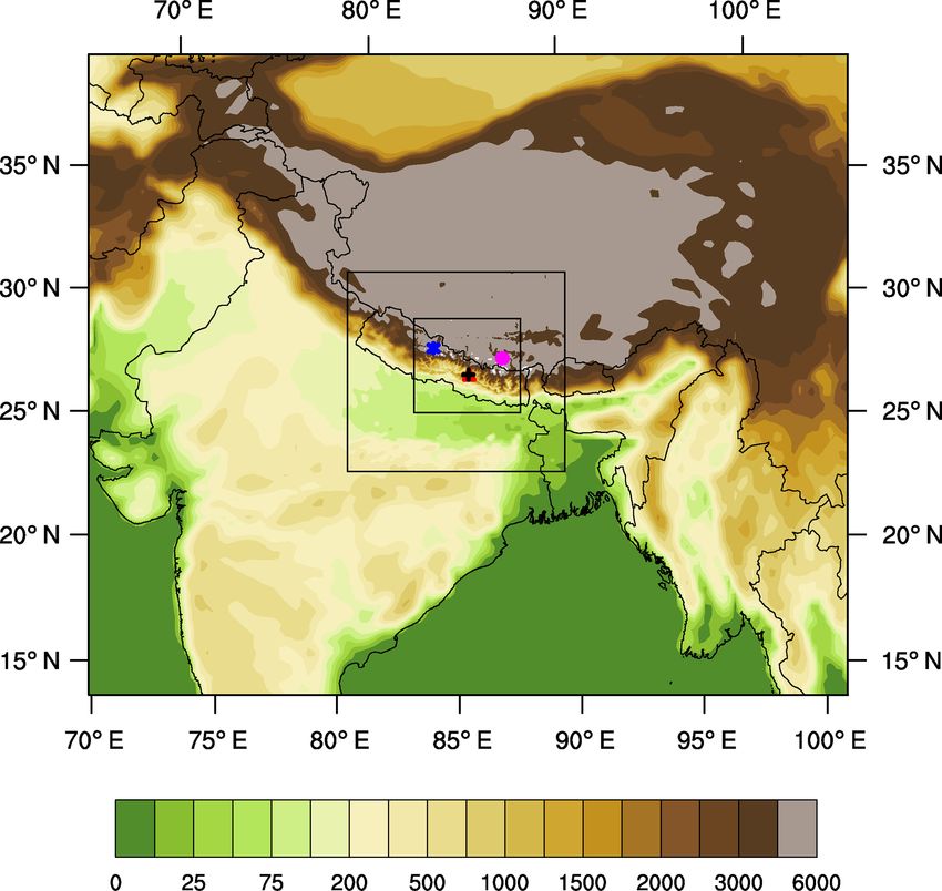
8212                                                                 M. Zhong et al.: Vehicle and brick kiln emissions in Nepal

Figure 1. Nested model domains with the terrain heights in meters (color shaded) and the locations of four measurement sites: Jomsom,
Nepal (blue asterisk); QOMS_CAS, China (pink dot); Bode, Nepal (red triangle); and the Tribhuvan International Airport, Nepal (black
cross).

Table 1. Description for each emissions scenario in 2015.

                     Emissions scenario      Description
                     HTAP                    Original HTAP_v2.2 emissions inventory
                     HTAP_vehicle            Original HTAP_v2.2 + updated vehicle emissions
                     HTAP_vehicle_brick      Original HTAP_v2.2 + updated vehicle emissions + brick kiln emissions

tors, and the distance traveled or the total starts for each of       as ambient temperature and relative humidity, were obtained
the vehicle categories. We classified vehicles into six over-         from Weather Underground for April 2015. Driving char-
all categories (motorcycles, buses, cars, trucks, taxis, and          acteristics for motorcycles, buses, taxis, and three-wheelers
three-wheelers), numerous technology-based subcategories,             were adopted from surveys in the Kathmandu Valley, docu-
and two fuel types (gasoline and diesel). For fuel quality in-        mented by Shrestha et al. (2013). Since we lack survey data
put values, we used unleaded gasoline with a sulfur content           for trucks and cars in Kathmandu, we used the data from
of 300 ppm and diesel with a sulfur content of 500 ppm. The           Pune, India, for these two types of vehicles (Barth et al.,
base emissions factors are derived from emissions tests con-          2007). Pune was the only representative city within South
ducted mainly in the USA, along with data collected in devel-         Asia, where the International Sustainable Systems Research
oping countries. The correction factors consider local con-           Center (ISSRC) conducted a detailed study of vehicle ac-
ditions (meteorology, altitude, inspection/maintenance pro-           tivity. The travel distances were obtained from the vehicle
gram, etc.), fuel quality, and power and driving characteris-         registration number and vehicle kilometers traveled (VKTs).
tics (vehicle specific power pattern, road grade, air condition-      Daily VKT and the number of starts per day were adopted
ing usage, and start pattern). Local meteorology data, such           from Shrestha et al. (2013), which is specific for vehicles in

Atmos. Chem. Phys., 19, 8209–8228, 2019                                                 www.atmos-chem-phys.net/19/8209/2019/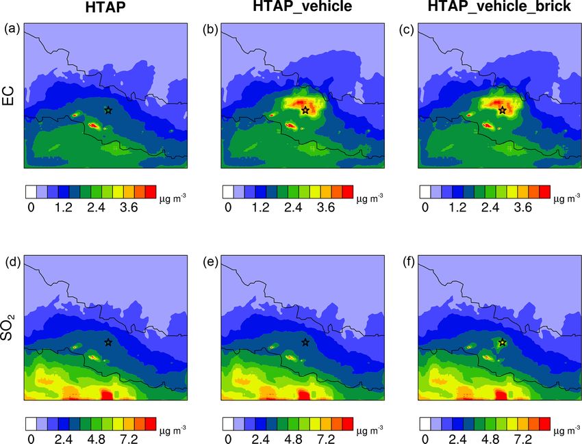
M. Zhong et al.: Vehicle and brick kiln emissions in Nepal                                                                                         8213

Table 2. Number of vehicles, daily mileage, and starts for vehicles                     2.2.3   Brick kiln emissions
in the Bagmati Zone, Nepal, in 2015.
                                                                                        We identified the kiln types in the Kathmandu Valley by com-
 Vehicle category                   Number of        Daily VKT           Number of      paring the specific images of brick kiln types with Google
                                vehicles, 2015a      (km d−1 )b       starts per day    Earth images dated April 2015. The monthly emissions of
 Motorcycle                              722 695               15                 3.8   compound i (Ei,j , g month−1 ) for a certain type of brick j
 Bus/mini bus                             20 207               96                   9   were calculated as the product of the amount of fuel con-
 Taxi                                      6206                87                  15   sumed (BKj , kg-fuel) and the corresponding emissions fac-
 Car/pickup/jeep                         136 391               44                  15   tor (EFi,j , g kg-fuel−1 ):
 Van/microbus                              2123                42                10.3
 Three-wheeler (tempo)                     2528                63                  12
                                                                                        Ei,j = BKj × EFi,j .                                         (1)
 Truck/mini-truck                         18 917              107                   9
a We obtained the number of vehicles in 2015 from the Department of Transport,          The calculated emissions were mapped based on the location
Nepal. b VKT of truck/mini-truck are from Malla (2014).
                                                                                        of each kiln.
                                                                                           The amount of fuel burned for each brick kiln BKj is esti-
                                                                                        mated using the following formula:
the Kathmandu Valley. The number of vehicles in 2015 was
taken from the government report of the DoTM (2017). Data
                                                                                        BKj = Pj × Wbrick × Ebrick /Ufuel ,                          (2)
used for the number of vehicles and VKTs for each vehicle
category in 2015 are summarized in Table 2. Table S1 in the                             where Pj is the production of brick kiln j (number of bricks
Supplement lists the detailed technology of each category,                              produced per month per kiln), Wbrick is the average weight
fraction of vehicles with different technology in fleet, and                            of a brick (kg brick−1 ), Ebrick is the specific energy con-
corresponding European vehicle emissions standards (Euro                                sumption of a brick (MJ kg−1 ), and Ufuel is the specific en-
Standards).                                                                             ergy density of fuel (MJ kg-fuel−1 ). Since the production of
   We used the IVE model to estimate emissions of CO, NOx ,                             each brick kiln was not available, we estimated the monthly
NMVOC, SO2 , PM, and some greenhouse gases. All emitted                                 mean production using one-sixth of the annual average pro-
PM was assumed to be PM2.5 because the ratio of PM2.5 to                                duction, as brick kilns in the Kathmandu Valley usually op-
PM10 is 0.92 for diesel vehicles and 0.88 for gasoline vehi-                            erate 6 months a year. The annual mean production was ob-
cles in the EPA 2014 MOVES model. Studies such as Gillies                               tained from a report submitted to the government of Nepal
et al. (2001) and Handler et al. (2008) have also found that                            (SMS Environment and Engineering Pvt. Ltd, 2017). Most
74 % and 67 % of PM10 is PM2.5 in on-road studies. Al-                                  brick kilns in the Kathmandu Valley are fueled by high-sulfur
though we understand that assuming all emitted PM10 to be                               coal (70 %), which is supplemented with sawdust (24 %), and
PM2.5 is potentially an overestimation, we believe that this is                         wood and other fuels (6 %) (Joshi and Dudani, 2008). Con-
acceptable, given the lack of observational data in Nepal or                            sidering that the dominant fuel for brick firing is coal and that
in South Asia.                                                                          the EFs used here correspond to emissions from coal-fueled
   Because the IVE model does not directly estimate emis-                               brick kilns, we used the specific energy density of coal to es-
sions of EC or OC, we used conversion factors derived from                              timate emissions. Values and references for each variable in
the study of Kim Oanh et al. (2010) to estimate these emis-                             Eq. (2) are presented in the Supplement (Table S2).
sions. Kim Oanh et al. (2010) specifically focused on the                                  EF values measured from a zigzag kiln during the NA-
emissions of diesel vehicles in developing countries and                                MaSTE field campaign are applied in Eq. (1) to calculate
tested a large number of vehicles. For vans, we used an                                 emissions estimates of various trace gases and PM. Table S1b
EC / PM mass ratio of 0.46 and OC / PM of 0.2, while for                                lists the species, associated EF, and references that we esti-
trucks and buses, we used EC / PM of 0.48 and OC / PM                                   mated the emissions for. We used EFs of a zigzag kiln rather
of 0.13. We collected a group of these conversion factors                               than a clamp kiln for all types of kilns in the valley because
from different studies in Table S3. Our EC / PM mass ratio is                           zigzag is the most common kiln type identified in the val-
close to the median value of all the studies listed below. The                          ley. We will provide more accurate emissions estimates in
total vehicle emissions from IVE were distributed spatially                             our emissions inventory when EFs of different types of kilns
and temporally based on HTAP_v2.2. While we acknowl-                                    become available.
edge that using conversion factors from one study ignores
the potential uncertainty due to driving pattern, weather con-                          2.2.4   Other emissions
ditions, fuel quality, and vehicle characteristics, we also feel
that our estimate provides a good middle ground, given the                              Anthropogenic emissions of other gaseous pollutants (CO,
existing study results.                                                                 NOx , NH3 , SO2 , and NMVOCs) and PM (EC, OC, PM2.5 ,
                                                                                        and PM10 ) from major sectors are taken from HTAP_v2.2
                                                                                        for 2010. HTAP_v2.2 is the most recent global emissions in-
                                                                                        ventory that includes emissions from various sectors such as

www.atmos-chem-phys.net/19/8209/2019/                                                                    Atmos. Chem. Phys., 19, 8209–8228, 2019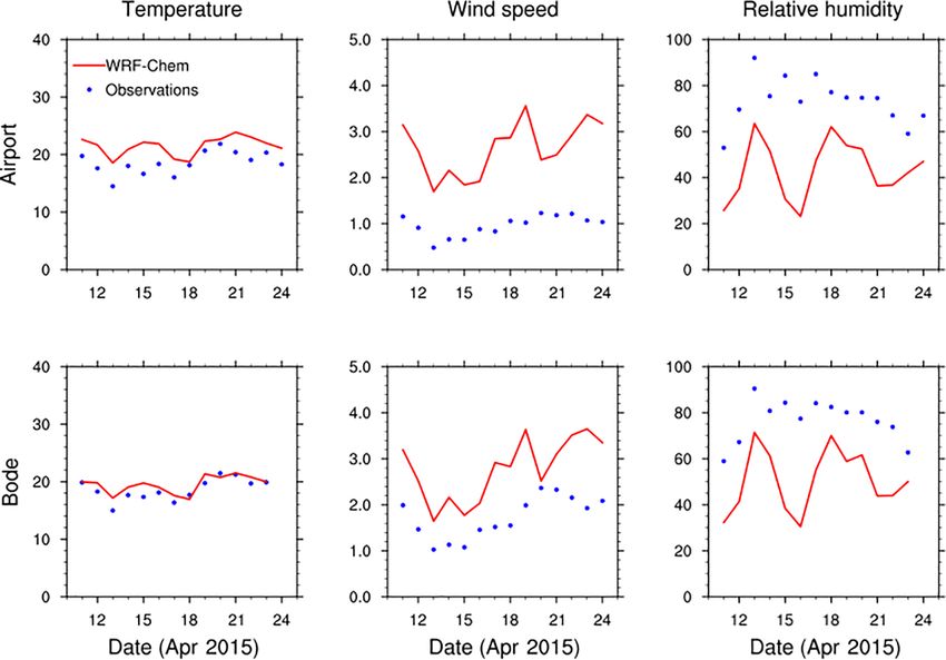
8214 M. Zhong et al.: Vehicle and brick kiln emissions in Nepal
energy, industry, agriculture, residential (including both heat- The overall performance of WRF-Chem in simulating me-
ing and cooking), aircraft, and shipping and has the highest teorological data and air pollutants against observations was
spatial resolution. However, as mentioned earlier, HTAP does evaluated using the correlation coefficient (r), the normal-
not currently include brick kiln emissions in their estimates ized mean bias (NMB), the mean fractional bias (MFB), the
and it also excludes large-scale biomass burning and crop mean fractional error (MFE), and the root-mean-square error
residue burning. For nonresidential “open” biomass burning (RMSE). The evaluation is based on 2-week statistics using
emissions, we therefore used emissions from the Fire IN- the daily mean values weighted for the day and night sam-
ventory from NCAR (FINN) inventory for the year 2015 pling times at each site.
(Wiedinmyer et al., 2011). For biogenic emissions, we used
the Model of Emissions of Gases and Aerosols from Na-
ture (MEGAN) version 2.1 (Guenther et al., 2012). Dust 3 Emissions comparison
emissions are calculated online, using the AFWA emissions
3.1 Vehicle emissions
scheme, as described above.
The numbers, mileage, and starts for different vehicle types
2.3 Observations and statistical methods for
in the Kathmandu Valley, based on the vehicle registration in-
comparisons
formation, are summarized in Table 2. Using the IVE model,
We compared our simulations with the surface observations we estimated monthly vehicle emissions for CO, SO2 , NOx ,
of air temperature, relative humidity, and wind speed at two NMVOCs, EC, OC, and PM2.5 (Table 3). Relative to the ve-
sites in the Kathmandu Valley. The meteorological data at hicle emissions estimates for 2010 by Shrestha et al. (2013),
the Bode site at a height of 23 m were collected during the our estimates are about 2 to 4 times higher due to (1) the in-
NAMaSTE field campaign and the data at the Tribhuvan In- creases in numbers of vehicles between 2010 and 2015, and
ternational Airport site at standard meteorological monitor- (2) the inclusion of diesel trucks that were not considered in
ing heights (2 m for air temperature and relative humidity, the earlier study. The total number of vehicles in this study
and 10 m for wind speed and direction) were provided by the is about 70 % higher than that of Shrestha et al. (2013). In
Department of Hydrology and Meteorology of the Ministry addition, the estimated running EFs for trucks are the highest
of Population and Environment of the government of Nepal. among seven categories of vehicles for all air pollutants, with
The Bode site is located in the eastern part of the Kathmandu values 4 to 5 times higher than those for buses, which ranked
Valley at a latitude of 27.689◦ N and longitude of 85.395◦ E. the second highest (Tables S0 and S1). Although trucks ac-
The altitude is about 1337 m. The airport is approximately count for only 2.3 % of the total numbers of vehicles, they are
4 km west of Bode (Fig. 2), at approximately the same alti- the major contributor to pollutant emissions due to their sub-
tude. stantially higher EFs. Trucks account for more than 80 % of
The daily ground-based AOD values at 550 nm were ob- monthly total emissions for both PM2.5 and NOx , and 50 %
tained from the AErosol RObotic NETwork (AERONET). or more for the other pollutants.
We used Level 2.0 for the QOMS_CAS site in China and Comparison of these new emissions estimates with those
the Level 1.5 for the Jomsom site in Nepal. In addition, we from the ground transport sector in the HTAP_v2.2 emissions
also compared the space-based AOD values retrieved from inventory reveals that CO, NOx , NMVOCs, EC, OC, and
the MODerate Resolution Imaging Spectrometer (MODIS) PM2.5 are significantly underestimated in HTAP (Table 3).
instrument aboard the Terra satellite with the simulated AOD For example, the emissions estimates of PM2.5 , OC, and EC
from WRF-Chem. MODIS provides AOD retrievals at a res- calculated using the IVE model were factors of 186, 100,
olution of 10 km ×10 km. In this study, we used Level 2 and and 375, respectively, greater than those in HTAP. In con-
Collection 6 aerosol optical thickness at 550 nm. Concentra- trast, SO2 emissions estimates agreed well and only differed
tions of EC and SO2 at Bode, Kathmandu, were sampled at a by 17 %. Our revised emissions of PM2.5 , EC, CO, and NOx
height of 20 m during the NAMaSTE field campaign on 12– from vehicles drive the substantially greater total emissions
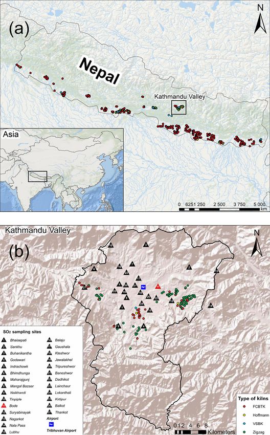
24 April 2015. We also compared simulated and observed of these species in the Bagmati Zone relative to those based
surface SO2 concentrations at several other sites in the val- on the HTAP (Fig. 3).
ley (Kiros et al., 2016). The observed surface SO2 is 8-week
3.2 Brick kiln emissions
mean concentrations between 23 March and 18 May 2013
from Kiros et al. (2016). They were measured at 15 sites We found 112 brick kilns in the Kathmandu Valley, con-
in the valley, including five urban sites (Bode, Indrachowk, sistent with a previously reported total of 110 (SMS Envi-
Maharajgunj, Mangal Bazaar, Suryabinayak), four suburban ronment and Engineering Pvt. Ltd, 2017). Figure 2 shows
sites (Bhaisepati, Budhanilkantha, Kirtipur, Lubhu), and six the spatial distribution of these brick kilns. Approximately
rural sites (Bhimdhunga, Nagarkot, Naikhandi, Nala Pass, 40 % of brick kilns are located in the southern portion of
Sankhu, Tinpiple) (Kiros et al., 2016). the valley, 35 % in the eastern portion, and the rest are in
the western portion. We identified four types of brick kilns,
Atmos. Chem. Phys., 19, 8209–8228, 2019 www.atmos-chem-phys.net/19/8209/2019/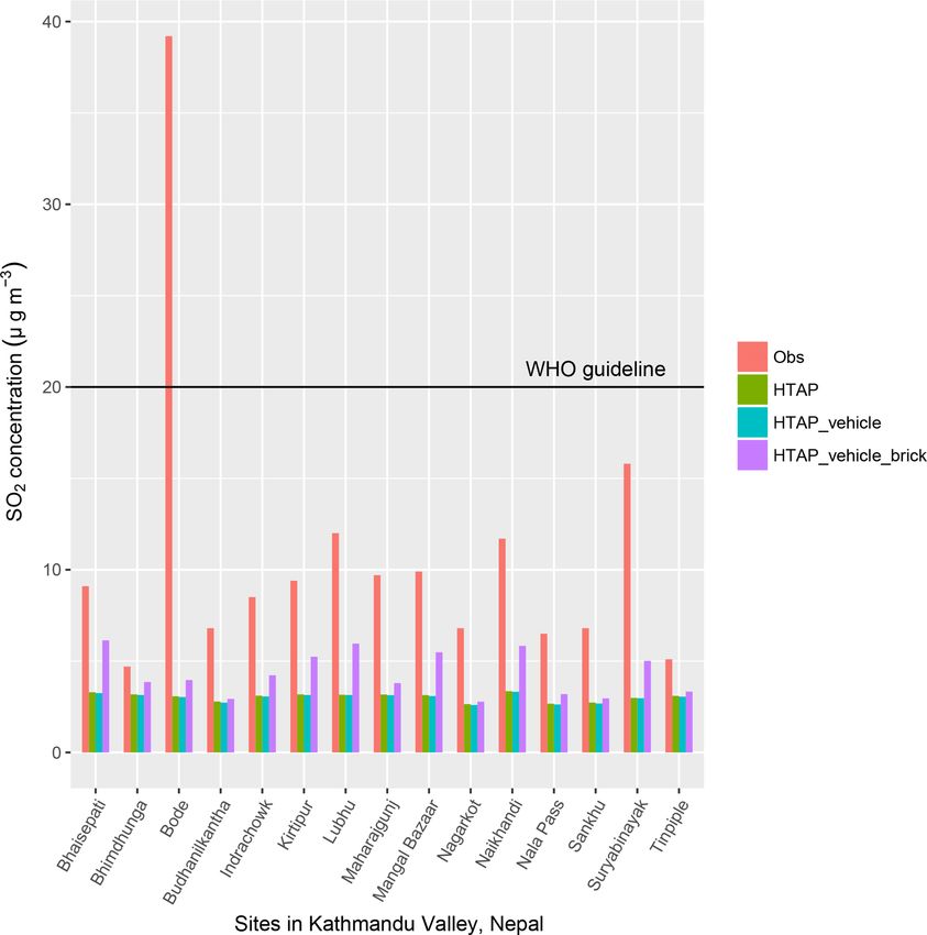
M. Zhong et al.: Vehicle and brick kiln emissions in Nepal                                                                        8215

Figure 2. Spatial distribution of brick kilns in Nepal (a) and Kathmandu Valley (b). Red, orange, blue, and green dots denote the fixed-
chimney Bull’s trench kiln (FCBTK), Hoffmann kiln, vertical shaft brick kiln (VSBK), and zigzag kiln, respectively.

www.atmos-chem-phys.net/19/8209/2019/                                                   Atmos. Chem. Phys., 19, 8209–8228, 2019
8216                                                                M. Zhong et al.: Vehicle and brick kiln emissions in Nepal

Figure 3. The monthly mean surface emissions of five pollutants, PM2.5 , EC, CO, NOx , and SO2 , from all sources in April 2015 used in
WRF-Chem for the three simulations. The star indicates the location of the Bode site.

Atmos. Chem. Phys., 19, 8209–8228, 2019                                                 www.atmos-chem-phys.net/19/8209/2019/
M. Zhong et al.: Vehicle and brick kiln emissions in Nepal 8217
Table 3. Total emissions from vehicles, brick kilns in the Kathmandu Valley during April 2015 estimated by this study versus corresponding
emissions from vehicles, and all sources considered in HTAP emissions inventory.
Unit (t month−1 ) CO SO2 NOx NMVOCs EC OC PM2.5
Total vehicle emissions, this study 6551 41 6152 1413 827 234 1852
Total brick kilns emissions, this study 98 123 13 13 1.08 10 135
Total emissions from all sectors, this study 18 668 308 6565 3978 976 839 2796
Total transport sector emissions in HTAP, 2010 188 35 80 98 2.2 2.3 10
Total emissions from all sectors in HTAP, 2010 12 207 179 479 2651 150 598 819
including FCBTK, Hoffmann kiln, vertical shaft brick kiln humidity with a correlation of 0.5–0.6 and NMB of −40.8 %
(VSBK), and zigzag kiln. Out of the 112 kilns, the domi- to −34.0 %, due to an underestimation of both minima and
nant types were zigzag (63) and FCBTK (46), while there maxima. In a previous WRF-Chem study in the Kathmandu
were only three Hoffmann kilns and VSBK kilns combined. Valley (Mues et al., 2018), an underestimation of relative hu-
Based on Eq. (2), the average fuel consumption of these kilns midity was also clearly observed near the ground. The tem-
was about 9700 t month−1 or 58 200 t yr−1 , which is close to poral correlation coefficient of daily 10 m wind speed is 0.7
65 100 t yr−1 estimated in a previous report (SMS Environ- at the airport and 0.8 at Bode. Although the model reproduces
ment and Engineering Pvt. Ltd, 2017). the daily variability well, it overestimates the wind speed at
Table 3 summarizes the estimated monthly total emis- both sites. The model performs better at Bode (NMB = 67 %)
sions of major air pollutants from brick kilns in the Kath- than at the airport site (NMB = 176 %) in simulating wind
mandu Valley. Of these species, those with the greatest speed. The modeled mean wind speed at the airport site is
mass emitted were PM2.5 (135 t month−1 ), followed by SO2 about 1.68 m s−1 higher than the observation, with a RMSE
(123 t month−1 ) and CO (98 t month−1 ), while emissions for of 1.74 m s−1 . WRF-Chem usually has difficulty simulating
other pollutants were less than 20 t month−1 . Table 3 also wind speed over complex mountain terrains; a larger bias
compares emissions from brick kilns and those from all other over mountain regions was also found in previous studies
sectors in the HTAP_v2.2 emissions inventory. Our brick kiln (Mar et al., 2016; Mues et al., 2018). Zhang et al. (2013)
SO2 and PM2.5 emissions estimates are each equivalent to explained that the overestimation in wind speeds is likely
68 % and 16 %, respectively, of the total emissions in the caused by poor representation of surface drag exerted by un-
HTAP estimates. The increase in PM2.5 and SO2 emissions resolved topographical features in WRF-Chem. A closer look
due to adding the brick kiln emissions can be seen clearly at the wind observational data reveals the presence of a lo-
in Fig. 3. For EC, OC, CO, NOx , and NMVOCs, the brick cal, thermally driven diurnal wind circulation that controls
kiln sector contribution is less than 3 % of our updated total the airflow regime in the Kathmandu Valley during weak
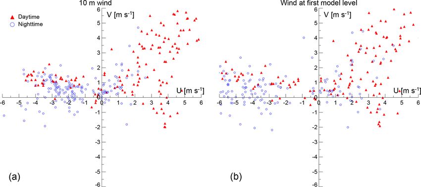
emissions. gradient synoptic-scale flow and arguably significantly im-
pacts the air quality in the valley (Fig. 5). During the day,
the winds at both Bode and the airport are predominantly
4 Model results and evaluation from the SW quadrant along the axis of the nearby river, with
hourly-averaged magnitudes of up to 5 m s−1 . In contrast, the
4.1 Meteorology katabatic winds during the night are much weaker, gener-
ally under 1 m s−1 and with a prevailing easterly component.
The different emissions scenarios did not impact simulated Note that winds at Bode are consistently stronger than those
meteorological conditions. Therefore, we only present the at the airport. One of the most likely reasons for that is the
statistical analysis of our HTAP_vehicle_brick simulation, differing measurement height at both sites: 23 m above sur-
using the HTAP inventory with updated emissions for both face at Bode and 10 m at the airport.
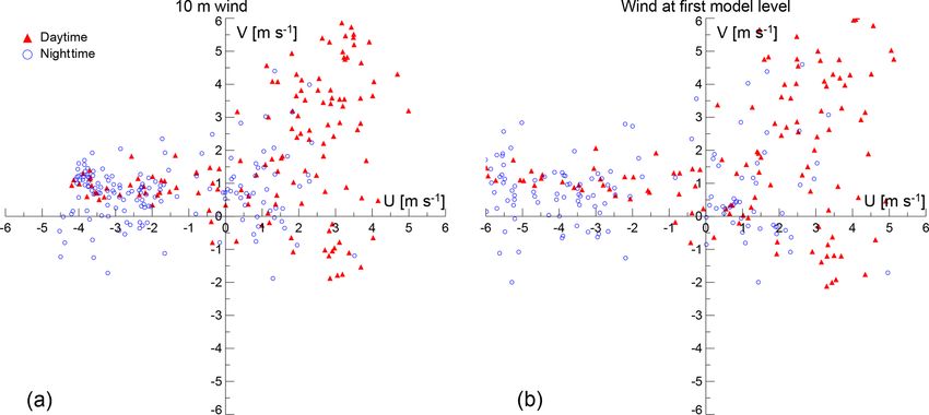
vehicles and brick kilns. Model-simulated 2 m temperature The model generally reproduces the wind direction shift at
and relative humidity, as well as 10 m wind speed, are com- both sites quite well (Figs. 6 and 7); however, the wind speed
pared to observations at two sites in the Kathmandu Val- magnitude is substantially overpredicted. The overestimation
ley: Bode and the Tribhuvan International Airport. Figure 4 is not that large during the day but it is severe during the
shows the comparisons of predicted daily-averaged quanti- nighttime hours, suggesting serious differences in the struc-
ties with observations and Table 4 presents the statistical in- ture of simulated and observed nighttime boundary layers.
dices of comparisons for each site. The temperature at Bode We should note here that the model does not directly predict
is simulated with a correlation of 0.8 and a small negative the wind field at 10 m height; instead it is extrapolated from
NMB of 4.7 %. At the airport, the correlation of 0.7 is close the first model level using Monin–Obukhov similarity theory
to that at Bode, but a larger bias is observed, with NMB
of 15.8 %. The model systematically underestimates relative
www.atmos-chem-phys.net/19/8209/2019/ Atmos. Chem. Phys., 19, 8209–8228, 2019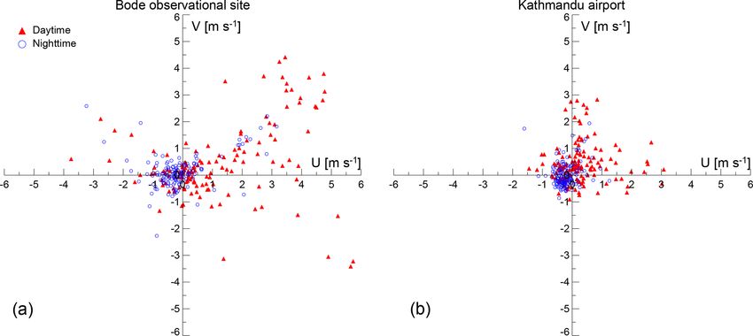
8218                                                                   M. Zhong et al.: Vehicle and brick kiln emissions in Nepal

Table 4. Statistical performance of model simulation for daily surface temperature, 10 m wind speed, and surface relative humidity at the
Tribhuvan International Airport (Airport) and Bode.

                                           Surface temperature (◦ C)    10 m wind speed (m s−1 )      Surface RH (%)
                  Statistical metrics
                                             Airport           Bode     Airport            Bode      Airport        Bode
                            Observation         18.6           18.7         1.0              1.7        73.3         76.9
               Mean
                            Modeled             21.5           19.6         2.6              2.8        43.5         50.7
                            Observation    14.5/21.9       15.0/21.5    0.5/1.2          1.0/2.4   53.0/92.1    59.0/90.5
               Min–max
                            Modeled        18.6/23.9       17.0/21.6    1.7/3.6          1.7/3.7   23.2/63.5    30.6/71.5
                      Mean bias                  2.9             0.9       1.7               1.1      −29.9        −26.2
                      NMB (%)                   15.8             4.7     176.0              61.2      −40.8        −34.0
                       RMSE                      3.2             1.3       1.7               1.1       32.0         28.2
                      Correlation                0.7             0.8       0.7               0.8        0.5          0.6

Figure 4. Comparisons of observed (blue dots) and modeled (red lines) daily mean 2 m temperature, 10 m wind speed, and 2 m relative
humidity at two sites (Airport and Bode) in the Kathmandu Valley.

(Jimenez et al., 2012), and therefore is highly influenced by           observed by MODIS and the modeled AOD at the 550 nm
the PBL scheme used in the simulations.                                 wavelength. In general, the simulated AOD values are higher
                                                                        in the southern part of the domain than those in the north-
4.2    AOD                                                              ern part. MODIS AOD also shows a similar spatial distribu-
                                                                        tion in the southern part but most data in the northern part
AOD is a column-integrated measurement and, thus, not di-               are missing due to cloud coverage. It is clear from the figure
rectly correlated with concentrations of near-surface PM.               that adding brick kiln emissions has little impact on AOD
However, in the context of model validation, AOD is use-                in the Kathmandu Valley, while modifying vehicle emissions
ful as a general indicator of near-surface air quality. Fig-            leads to a significant increase in modeled AOD. The average
ure 8 depicts the spatial pattern of the 2-week mean AOD

Atmos. Chem. Phys., 19, 8209–8228, 2019                                                  www.atmos-chem-phys.net/19/8209/2019/
M. Zhong et al.: Vehicle and brick kiln emissions in Nepal 8219 Figure 5. Hourly-averaged observed U- and V-wind components during the period of 11–24 April at the (a) Bode site and (b) Tribhuvan International Airport. Daytime winds are shown with red closed triangles and the open blue circles denote winds during the night. Note that the winds at the Bode site and the airport are measured at a height of 17 and 10 m above the surface, respectively. Figure 6. Hourly-averaged simulated U- and V-wind components during the period of 11–24 April: (a) at 10 m height above surface and (b) at the first model level (28 m height) at the model grid point closest to the Bode site. Daytime winds are shown with red closed triangles and the open blue circles denote winds during the night. difference in AOD between the simulations with and with- peak on 14 April, when the observed AOD is near 1.0, an in- out the revised vehicle emissions is 18 % in the Kathmandu dication of severe air pollution. Instead, our model predicts a Valley. As discussed in Sect. 3.2, diesel engines emit a large somewhat lower peak on the preceding day. This high AOD amount of EC. These aerosols strongly absorb sunlight at all value was driven by emissions from a wildfire located south- UV–vis wavelengths and, consequently, contribute to higher east of Jomsom. It can be seen clearly from the model simu- AOD values. lation (Fig. S1) that the fire caused high surface PM and CO The time series of simulated versus observed daily mean concentrations near the burning area on 12 April. Since the AOD at the two AERONET sites within the model domain prevailing wind direction on 13 April in the simulation was (Jomsom, Nepal and QOMS_CAS, China) and the corre- from the southeast and with the overestimated wind speed, sponding performance statistics are presented in Fig. 9. The the smoke was transported to the northwest and increased model tends to overestimate the lower observed values at the simulated AOD value at the Jomsom site earlier than ob- the QOMS_CAS site, with an MFB of 56 %. At Jomsom, served. the model predicts the lower measured AOD values reason- ably well during 15–24 April. However, the model misses the www.atmos-chem-phys.net/19/8209/2019/ Atmos. Chem. Phys., 19, 8209–8228, 2019
8220                                                                    M. Zhong et al.: Vehicle and brick kiln emissions in Nepal

Figure 7. Same as Fig. 6 but for the model grid point closest to the Tribhuvan International Airport.

4.3    EC                                                                turbance. During that period, the wind speeds are generally
                                                                         below 2 m s−1 even during the day, suggesting that the peak
Figure 10 shows the spatial pattern of simulated EC, aver-               in the surface concentrations (Fig. 11) could be related to
aged during the simulation period. The average simulated EC              suppressed boundary-layer mixing.
concentration in the Kathmandu Valley during the 2-week                     Observed EC concentrations are strongly underestimated
simulation period was approximately 6.2 µg m−3 , higher than             with poor correlation when the original HTAP emissions are
concentrations in the surrounding regions. Vehicles (primar-             used as model input (MFB = −125 %, r = 0.19 for 24 h aver-
ily diesel trucks and buses) contribute approximate 85 % of              aged EC, Table 5). This is similar to Mues et al. (2018), who
total EC emissions, whereas brick kilns account for only                 reported an underestimation of EC concentrations by a factor
about 0.11 %. Consequently, the simulation that includes                 of 5 when using HTAP emissions in their simulations. The
brick kiln emissions (HTAP_vehicle_brick) does not im-                   simulation with updated vehicle emissions (HTAP_vehicle)
prove the model performance in predicting EC at Bode rela-               shows reduced bias and better correlation (MFB = −73 %,
tive to that with updated vehicle emissions (HTAP_vehicle).              r = 0.61 for 24 h average), although the model still underes-
   Figure 11 depicts the time series of observed and sim-                timates EC concentrations.
ulated surface EC concentrations. The average EC con-                       The model captures the daytime low concentrations very
centration observed at Bode during the campaign was                      well during 18–21 April, but it fails to predict the observed
5.6 µg m−3 during daytime, 10.82 µg m−3 during nighttime,                peak on 15–16 April. Such high EC concentration episodes
and 8.32 µg m−3 for the 24 h average. Two factors con-                   can be caused by either stagnant meteorological conditions
tributed to the nighttime increase in surface concentrations:            or enhanced emissions. We examined the precipitation and
(1) the diminishing mixing-layer depth and (2) the air flow              wind speed at Bode during the high and low episode peri-
circulation shift in response to surface cooling. As the night           ods (Table S2). On 16 (high EC) and 19 April (low EC), no
progresses, the turbulent mixing in the developing nocturnal             rainfall was observed. The daytime wind speed on 16 April
boundary layer is suppressed and air pollutants are confined             (2.4 m s−1 ) was slightly lower than that on 19 April (2.7 m−1 )
in a shallow layer close to surface. The shift in the wind               but the EC concentration on 16 April was 6 times higher. This
direction is also conducive to increased surface concentra-              suggests that a sporadic emissions source (e.g., garbage or
tions as the Bode site is located downwind with respect to               biomass burning) that was not accounted for in our model
the major cluster of brick kilns in the area (Figs. 2 and 5).            could be responsible for the observed high concentration
In contrast, during daytime the mixing-layer depth increases             episode.
in response to solar heating and promotes the vertical mixing               The nighttime surface concentrations are significantly un-
throughout the depth of the whole boundary layer, leading to             derestimated by the model throughout the entire period.
a notable decrease in surface concentrations. The Bode site              One possible cause for this underestimation is illustrated in
during the day is also upwind from the brick kiln cluster,               Fig. S2, showing the diurnal evolution of the modeled mixing
which leads to further reduced concentrations. This idealized            layer height. During the night, the simulated boundary layer
scenario holds true for most of the simulation period with               remains well mixed up to a height of 500 m, which facilitates
the exception of the days between 13 and 16 April, when the              the vertical transport of pollutants, and consequently, leads
local air flow circulation is disrupted by a large-scale dis-            to lower surface concentrations.

Atmos. Chem. Phys., 19, 8209–8228, 2019                                                     www.atmos-chem-phys.net/19/8209/2019/
M. Zhong et al.: Vehicle and brick kiln emissions in Nepal 8221 Figure 8. The 2-week average AOD: (a) retrieved from the MODIS Terra satellite, (b) simulated using WRF-Chem with original HTAP emissions, (c) simulated using WRF-Chem with HTAP with updated vehicle emissions, and (d) simulated using WRF-Chem with HTAP emissions plus updated vehicles and brick kiln emissions. The star indicates the location of the Bode site. www.atmos-chem-phys.net/19/8209/2019/ Atmos. Chem. Phys., 19, 8209–8228, 2019
8222                                                                 M. Zhong et al.: Vehicle and brick kiln emissions in Nepal

Figure 9. Comparisons of observed (blue dots) and modeled (red lines) daily mean AOD at two AERONET sites (QOMS_CAS and Jomsom).

Figure 10. The 2-week average surface EC (a, b, c) and SO2 (d, e, f) concentrations obtained from three simulations: HTAP, HTAP_vehicle,
and HTAP_vehicle_brick. The star indicates the location of the Bode site.

Atmos. Chem. Phys., 19, 8209–8228, 2019                                                 www.atmos-chem-phys.net/19/8209/2019/
M. Zhong et al.: Vehicle and brick kiln emissions in Nepal                                                                        8223

Figure 11. Comparisons of observed (blue dots) and modeled EC concentrations in the daytime and nighttime and daily mean for the three
scenarios at Bode. Observed values are taken during the NAMaSTE campaign (Jayarathne et al., 2018)

Table 5. Statistical measures calculated for three model simulations with different emissions inputs for EC. Obs (µg m−3 ) and model
(µg m−3 ) are 2-week mean daily average values of observed and modeled EC, respectively. r is correlation coefficient between observa-
tion and model simulations; NMB (%) is the normalized mean bias between observations and model simulations; MFB (%) and MFE (%)
are the mean fractional bias and mean fractional error; RMSE is the root-mean-square error between observations and the model (µg m−3 ).

           Emissions               Day/night     Obs    Model          r      MB       NMB         MFB       MFE     RMSE
                                   Day           5.60      1.34   −0.21     −4.27    −76.15     −107.71    107.71       5.49
           HTAP                    Night        10.82      1.61    0.12     −9.20    −85.08     −142.45    142.45      10.25
                                   24 h          8.32      1.48    0.19     −6.83    −82.19     −125.77    125.77       8.31
                                   Day           5.60      2.56     0.28    −3.04    −54.32      −58.74      60.62      4.47
           HTAP_vehicle            Night        10.82      3.77     0.48    −7.05    −65.17      −90.56      90.56      8.20
                                   24 h          8.32      3.19     0.61    −5.13    −61.66      −75.29      76.19      6.67
                                   Day           5.60      2.62     0.25    −2.99    −53.31      −56.68      58.52      4.44
           HTAP_vehicle_brick      Night        10.82      3.85     0.47    −6.97    −64.45      −88.69      88.69      8.13
                                   24 h          8.32      3.26     0.61    −5.06    −60.85      −73.33      74.21      6.62

   It is also possible that we might have underestimated the          4.4    SO2
EC emissions from the brick kilns near Bode. In our emis-
sions inventory we use an average kiln productivity to esti-
mate the emissions; thus if the productivities of these kilns         Figure 10 presents the 2-week average SO2 concentra-
are higher than the average, or if their efficiency is lower,         tions for the three simulations. The average SO2 concentra-
their emissions could have been underestimated in the in-             tion in the HTAP_vehicle_brick simulation is approximately
ventory. Another possibility is that additional sources are           3.6 µg m−3 in the Kathmandu Valley, higher than the sur-
still missing, for example, garbage burning, biomass burn-            rounding areas in Nepal. Revised vehicle emissions have lit-
ing, and/or diesel generators. Stockwell et al. (2016) found          tle impact on SO2 concentration in the valley, but brick kiln
that garbage burning in the Kathmandu Valley may produce              emissions contribute 50 % of simulated SO2 concentrations.
significantly more EC emissions than previously thought.              The 2-week mean SO2 concentration measured at the Bode
Due to power outages, especially in the dry season, the use           site was 39.7 µg m−3 . The model largely underestimates the
of generators was still prevalent in the valley in 2015. A            observation, with the modeled mean SO2 concentration of
study conducted by the World Bank (2014) found that nearly            5.3 µg m−3 . SO2 is mainly a primary pollutant, directly emit-
200 000 small power generators, powered by diesel, were               ted from sources. SO2 concentrations are highly related to
used for pervasive power shortages in Nepal. Nevertheless,            its emissions. The large discrepancy between the model sim-
these comparisons suggest that there is still a need for fur-         ulation and observation at this site is probably because our
ther improvement of constructing local emissions inventories          model resolution is not able to capture spatially concentrated
in the Kathmandu Valley.                                              high emissions of SO2 near Bode. Kiros et al. (2016) mea-
                                                                      sured SO2 concentrations at 15 sites in 8 weeks from March
                                                                      to May 2013 in the Kathmandu Valley and observed high

www.atmos-chem-phys.net/19/8209/2019/                                                   Atmos. Chem. Phys., 19, 8209–8228, 2019
8224 M. Zhong et al.: Vehicle and brick kiln emissions in Nepal Figure 12. Comparisons of modeled and observed SO2 concentrations at 14 sites in the Kathmandu Valley. The modeled SO2 is the 2-week mean daily SO2 concentrations averaged from 12 to 24 April 2015. The observed SO2 is the 8-week mean SO2 concentrations between 23 March and 18 May 2013 reported in the study of Kiros et al. (2016). SO2 concentrations close to brick kilns. In particular, the av- kilns when more information on individual brick kilns be- erage SO2 concentration measured at Bode was the highest comes available. (39.2 µg m−3 ) and 2–6 times higher than those at the other 14 Figure 12 compares modeled 2-week mean SO2 concen- sites (4.7–15.8 µg m−3 ) in the Kathmandu Valley. They ex- trations with observed 8-week mean SO2 measured between plained that the elevated surface SO2 concentration at Bode 23 March and 18 May 2013, reported in the study of Kiros is mainly caused by nearby brick kilns, which are fueled by et al. (2016). None of these sites exceeded the Nepal na- coal. We found that there are 12 brick kilns located within tional air quality standard of 70 µg m−3 for the 24 h mean, the 4 km distance from the Bode site. Although we have in- but SO2 concentrations at the Bode site were almost twice as cluded emissions of these brick kilns in our model inputs, we high as the WHO standard of 20 µg m−3 . Since our own NA- may still have overestimated dilution and/or underestimated MaSTE campaign only collected SO2 at the Bode site, we emissions from these brick kilns by using monthly average also included the study of Kiros et al. (2016) to illustrate the productivity and average emissions factors of zigzag brick magnitude difference in observational data at different loca- kilns. We hope to improve our emissions inventory of brick tions within the Kathmandu Valley. The 2-week mean SO2 Atmos. Chem. Phys., 19, 8209–8228, 2019 www.atmos-chem-phys.net/19/8209/2019/
M. Zhong et al.: Vehicle and brick kiln emissions in Nepal                                                                     8225

concentration from NAMaSTE in 2015 was 39.7 µg m−3 at            kilns contribute 68 % of the total SO2 emissions in the Kath-
Bode, while the 8-week mean in 2013 by Kiros et al. (2016)       mandu Valley in the HTAP_v2.2 inventory.
was 39.2 µg m−3 , showing similarities, giving us confidence        Using the original HTAP emissions results in large under-
that comparing the magnitude difference among sites was          estimations of both surface EC and SO2 in the Kathmandu
possible, despite the difference in observed years. We used      Valley. Our revised vehicle emissions significantly reduced
these 2013 measurements to represent the ambient SO2 con-        model bias and improved model–observation correlation for
centrations during our simulation period. Including brick kiln   surface EC concentrations. We found that surface EC con-
emissions improves model prediction of SO2 concentrations        centrations increased by 50 % on average due to our revised
at all sites. The simulated SO2 concentrations with brick kiln   on-road vehicle emissions estimates. Conversely, brick kiln
emissions are closer to observations compared with those         emissions contributed approximately 50 % of the modeled
without them, although the model still underestimates SO2 .      surface SO2 concentrations in the Kathmandu Valley. Al-
This underestimation is probably due to brick kiln SO2 emis-     though model performance has been enhanced considerably,
sions. We applied an emissions factor of 12.7 g kg−1 of fuel     by using revised vehicle emissions and by adding newly cre-
measured from zigzag kilns (Stockwell et al., 2016) to all       ated brick kiln emissions, the model still underestimates the
types of brick kilns. These were the only available observa-     observed EC by 73 % and SO2 by 87 % at the Bode site dur-
tional data in Nepal at the time of this study. A more recent    ing the simulation period. The large underestimation at Bode
study by Nepal et al. (2019) reported that the mean value of     could be a result of the site’s proximity to large point sources
the SO2 emissions factor from zigzag kilns is 24 ± 22 g kg−1     or assuming average EFs for these point sources, but addi-
of fuel, which is almost twice as high as that used in our       tional sources not included in our inventory could also be
study. If we doubled our SO2 emissions for brick kilns,          important for improving the model performance. More infor-
the modeled SO2 concentrations would be much closer to           mation on the production rates of individual brick kilns and
the observations. Assuming the linear relationship in SO2 ,      emissions factors for each major type of brick kiln could sig-
the average difference between the observed and modeled          nificantly improve the inventory and comparisons. It is im-
SO2 concentrations would drop from 4.4 to 2.8 µg m−3 . We        portant that the complex topography and meteorology with
plan to revisit our brick kiln emissions inventory as more       limited observational data limit the degree of model evalu-
emissions factors become available. Our study highlights         ation currently possible in the Kathmandu Valley. The con-
the importance of improving the emissions factor of SO2          centrations of pollutants are highly dependent on the mea-
for brick kilns in Nepal. The difference between observa-        surement locations and topography of their surroundings and
tion and model simulation ranges from 0.8 to 10 µg m−3 for       more observational data at a finer scale within the valley are
all sites except Bode where the difference is 34.4 µg m−3 .      essential to better evaluate the local chemical transport mod-
This result suggests that surface SO2 concentrations in the      els. Despite the uncertainties, the results here suggest that
Kathmandu Valley are highly variable and are influenced          emissions from brick kilns are substantial and current esti-
by nearby sources. Future simulations with a higher spatial      mates of emissions underestimate total emissions by omitting
model resolution and emissions inputs may help to resolve        this source.
the strong spatial gradients in SO2 concentrations.                 Our main objective was to improve the emissions invento-
                                                                 ries for on-road vehicles and brick kilns and assess the im-
                                                                 pacts of revised emissions on local air quality. Our results
                                                                 demonstrate that the existing emissions inventories need sig-
5   Summary and future work                                      nificant modification for the road transportation sector. Miss-
                                                                 ing sources in the Kathmandu Valley such as brick kilns are
In this paper, we modified the HTAP emissions inventory          also important in predicting local air quality. We suggest that
for Kathmandu’s road transport sector. We also developed         more efforts are needed to improve local emissions infor-
a point source emissions inventory for brick kilns in the        mation by updating emissions estimates from major sources
Kathmandu Valley, and examined the impacts of emissions          and developing an emissions inventory including underrep-
from on-road vehicles and brick kilns on local air quality for   resented sources, such as crop residue and garbage burning.
April 2015. Emissions from vehicles were updated using the       A more comprehensive and accurate emissions inventory al-
IVE model to reflect the most recent vehicle registration in-    lows the local government to identify and define key emis-
formation and the local vehicle technology and driving con-      sions sources in the Kathmandu Valley. The improved emis-
ditions in the Kathmandu Valley. We found that PM emis-          sions inventory is urgently needed to robustly evaluate the
sions from the road transport sector in the HTAP_v2.2 inven-     effectiveness of various future policies on emissions mitiga-
tory are largely underestimated. The IVE-estimated EC emis-      tion in this region.
sions are 375 times higher than those estimated in HTAP.
Our brick kiln emissions estimates were created to account
for one of the most important missing sources in the existing    Code availability. The WRF-Chem model is an open-source, pub-
emissions inventories. We found that emissions from brick        licly available, and continually improved software. Version 3.5 used

www.atmos-chem-phys.net/19/8209/2019/                                              Atmos. Chem. Phys., 19, 8209–8228, 2019
8226 M. Zhong et al.: Vehicle and brick kiln emissions in Nepal
in this study can be downloaded at http://www2.mmm.ucar.edu/ mos. Environ., 32, 2981–2999, https://doi.org/10.1016/S1352-
wrf/users/download/get_source.html (last access: 15 June 2019). 2310(98)00006-5, 1998.
Known problems of the WRF-Chem version 3.5 have been fixed, Angel, H. and Alisa, Z.: Environmental Perfor-
using solutions provided online at http://www2.mmm.ucar.edu/wrf/ mance Index, 1–5, American Cancer Society,
users/wrfv3.5/known-prob-3.5.html (last access: 15 June 2019). https://doi.org/10.1002/9781118445112.stat03789.pub2, 2016.
Barth, M., Davis, N., Lents, J., and Nikkila, N.: Vehicle Ac-
tivity Patterns and Emissions in Pune, India, Transporta-
Data availability. The NCEP GFS data used for this study are tion Research Record, Transp. Res. Record, 2038, 156–166,
from the Research Data Archive (RDA), which is maintained by https://doi.org/10.3141/2038-20, 2007.
the Computational and Information Systems Laboratory (CISL) Davis, N., Lents, J., Osses, M., Nikkila, N., and Barth, M.: Part 3:
at the National Center for Atmospheric Research (NCAR). The Developing Countries: Development and Application of an Inter-
data are available at https://doi.org/10.5065/D6FB50XD (Na- national Vehicle Emissions Model, Transp. Res. Record, 1939,
tional Centers for Environmental Prediction/National Weather Ser- 155–165, https://doi.org/10.3141/1939-18, 2005.
vice/NOAA/U.S. Department of Commerce, 1997). The gridded DoTM: Vehicle Registered in Bagmati Zone in Fiscal
brick kiln emissions data for the Kathmandu Valley are avail- Year 072-73, available at: https://www.dotm.gov.np/en/
able at https://esaikawa.files.wordpress.com/2019/06/kathmandu_ vehicle-registration-record/ (last access: 15 June 2019),
brick_kiln_emissions.xlsx (last access: 21 June 2019). 2017.
Emmons, L. K., Walters, S., Hess, P. G., Lamarque, J.-F., Pfis-
ter, G. G., Fillmore, D., Granier, C., Guenther, A., Kinnison,
Supplement. The supplement related to this article is available D., Laepple, T., Orlando, J., Tie, X., Tyndall, G., Wiedinmyer,
online at: https://doi.org/10.5194/acp-19-8209-2019-supplement. C., Baughcum, S. L., and Kloster, S.: Description and eval-
uation of the Model for Ozone and Related chemical Trac-
ers, version 4 (MOZART-4), Geosci. Model Dev., 3, 43–67,
https://doi.org/10.5194/gmd-3-43-2010, 2010.
Author contributions. MZ ran the model simulations and drafted
Gao, Y., Zhao, C., Liu, X., Zhang, M., and Leung, L. R.: WRF-
the paper. ES and AA contributed to the analysis and the writing
Chem simulations of aerosols and anthropogenic aerosol ra-
of all versions of the paper. CC and BS contributed to developing
diative forcing in East Asia, Atmos. Environ., 92, 250–266,
a new brick kiln emissions inventory for Nepal. WY contributed
https://doi.org/10.1016/j.atmosenv.2014.04.038, 2014.
to transport emissions analysis. WC, RJY, TJ, EAS, MR, and AKP
Gillies, J. A., Gertler, A. W., Sagebiel, J. C., and Dippel, W. A.:
provided observational data and support throughout the paper pro-
On-Road Particulate Matter (PM2.5 and PM1 0) Emissions in the
duction. All authors contributed to revising the paper.
Sepulveda Tunnel, Los Angeles, California, Environ. Sci. Tech-
nol., 35, 1054–1063, https://doi.org/10.1021/es991320p, 2001.
Gronskei, K. E., Gram, F., Hagen, L. O., and Larssen, S.: Urban Air
Competing interests. The authors declare that they have no conflict Quality Management Strategy in Asia (URBAIR): Kathmandu
of interest. valley report, Tech. Rep. 52906, World Bank, 1996.
Guenther, A. B., Jiang, X., Heald, C. L., Sakulyanontvittaya,
T., Duhl, T., Emmons, L. K., and Wang, X.: The Model of
Acknowledgements. Maheswar Rupakheti acknowledges support Emissions of Gases and Aerosols from Nature version 2.1
from the IASS, which is funded by the German Federal Ministry for (MEGAN2.1): an extended and updated framework for mod-
Education and Research (BMBF) and the Brandenburg State Min- eling biogenic emissions, Geosci. Model Dev., 5, 1471–1492,
istry for Science, Research and Culture (MWFK). https://doi.org/10.5194/gmd-5-1471-2012, 2012.
Guo, H., Zhang, Q. Y., Shi, Y., and Wang, D. H.: Evaluation of
the International Vehicle Emission (IVE) model with on-road
Financial support. This research has been supported by the Na- remote sensing measurements, J. Environ. Sci., 19, 818–826,
tional Science Foundation, Division of Atmospheric and Geospace https://doi.org/10.1016/S1001-0742(07)60137-5, 2007.
Sciences (grant nos. AGS-1350021, AGS-1349976, AGS-1351616, Handler, M., Puls, C., Zbiral, J., Marr, I., Puxbaum, H.,
and AGS-1355551). Additional support was provided by ICIMOD and Limbeck, A.: Size and composition of particulate
through a contract with the University of Virginia. emissions from motor vehicles in the Kaisermühlen-
Tunnel, Vienna, Atmos. Environ., 42, 2173–2186,
https://doi.org/10.1016/j.atmosenv.2007.11.054, 2008.
Review statement. This paper was edited by Sachin S. Gunthe and Janssens-Maenhout, G., Pagliari, V., and Muntean, M.: Global
reviewed by two anonymous referees. emission inventories in the Emission Database for Global At-
mospheric Research (EDGAR) – Manual (I): Gridding: EDGAR
emissions distribution on global grid maps, Tech. Rep. 25785,
JRC, 2013.
References Janssens-Maenhout, G., Crippa, M., Guizzardi, D., Dentener, F.,
Muntean, M., Pouliot, G., Keating, T., Zhang, Q., Kurokawa,
Ackermann, I. J., Hass, H., Memmesheimer, M., Ebel, A., J., Wankmüller, R., Denier van der Gon, H., Kuenen, J. J.
Binkowski, F. S., and Shankar, U.: Modal aerosol dynam- P., Klimont, Z., Frost, G., Darras, S., Koffi, B., and Li,
ics model for Europe: development and first applications, At-
Atmos. Chem. Phys., 19, 8209–8228, 2019 www.atmos-chem-phys.net/19/8209/2019/You can also read