LoopStructural 1.0: time-aware geological modelling - GMD
←
→
Page content transcription
If your browser does not render page correctly, please read the page content below
Geosci. Model Dev., 14, 3915–3937, 2021
https://doi.org/10.5194/gmd-14-3915-2021
© Author(s) 2021. This work is distributed under
the Creative Commons Attribution 4.0 License.

LoopStructural 1.0: time-aware geological modelling
Lachlan Grose1 , Laurent Ailleres1 , Gautier Laurent2 , and Mark Jessell3
1 School of Earth Atmosphere and Environment, Monash University, Melbourne 3800, Australia
2 Universitéd’Orléans, CNRS, BRGM, ISTO, UMR 7327, Orleans, France
3 Mineral Exploration Cooperative Research Centre, School of Earth Sciences, UWA, Perth 6907, Australia

Correspondence: Lachlan Grose (lachlan.grose@monash.edu)

Received: 6 October 2020 – Discussion started: 16 December 2020
Revised: 10 April 2021 – Accepted: 10 May 2021 – Published: 29 June 2021

Abstract. In this contribution we introduce LoopStructural,       faces in 3D geological models: (1) one in which the surface
a new open-source 3D geological modelling Python pack-            is represented by directly triangulating control points defin-
age (http://www.github.com/Loop3d/LoopStructural, last ac-        ing the surface geometry or (2) one in which the surface is
cess: 15 June 2021). LoopStructural provides a generic API        extracted as an isovalue or level set of an implicit function
for 3D geological modelling applications harnessing the core      (Wellmann and Caumon, 2018). Explicit surface representa-
Python scientific libraries pandas, numpy and scipy. Six dif-     tion in geological modelling refers to manually drawn sur-
ferent interpolation algorithms, including three discrete in-     faces and is usually time consuming and requires significant
terpolators and 3 polynomial trend interpolators, can be used     subjective user input because surfaces are usually sculpted
from the same model design. This means that different in-         to the modellers conceptual idea in a similar way to draw-
terpolation algorithms can be mixed and matched within a          ing polylines in geographical information systems or using
geological model allowing for different geological objects,       computer-aided design software. Implicit surface representa-
e.g. different conformable foliations, fault surfaces and un-     tion involves approximating an unknown function that repre-
conformities to be modelled using different algorithms. Geo-      sents the distance to a geological surface. The implicit func-
logical features are incorporated into the model using a time-    tion can be queried anywhere throughout the model for the
aware approach, where the most recent features are modelled       value or gradient of the function. The implicit function is fit-
first and used to constrain the geometries of the older fea-      ted to observations that are used to infer the geometry of a
tures. For example, we use a fault frame for characterising       geological surface, for example the distance to the geological
the geometry of the fault surface and apply each fault se-        surface (for stratigraphic horizons this may be the cumula-
quentially to the faulted surfaces. In this contribution we use   tive thickness) or the gradient of the function (on contact or
LoopStructural to produce synthetic proof of concepts mod-        off contact) observations. The topological relationships be-
els and a 86 km × 52 km model of the Flinders Ranges in           tween different geological features, e.g. horizons, faults in-
South Australia using map2loop.                                   teractions, intrusions and unconformities, are incorporated
                                                                  using multiple implicit functions for different components of
                                                                  the model. Implicit surface representation removes the need
                                                                  to generate surfaces and allows for the geological features to
1   Introduction                                                  be represented directly by the implicit function value.
                                                                     All implicit surface modelling techniques involve finding a
Understanding and characterising the geometry and inter-          combination of weighted basis functions that fit the geolog-
action between geological features in the subsurface is an        ical observations. There are two main approaches used for
important stage in resource identification and management.        implicit surface modelling: (1) data-supported approaches
A surface or combination of surfaces can be used to repre-        where the basis functions are estimated at the data points
sent the subsurface geometry of geological features or struc-     (Calcagno et al., 2008a; Cowan et al., 2003; Gonçalves et
tural elements within 3D geological models (Caumon et al.,        al., 2017; Hillier et al., 2014; Lajaunie et al., 1997) and
2009). There are two main approaches for representing sur-

Published by Copernicus Publications on behalf of the European Geosciences Union.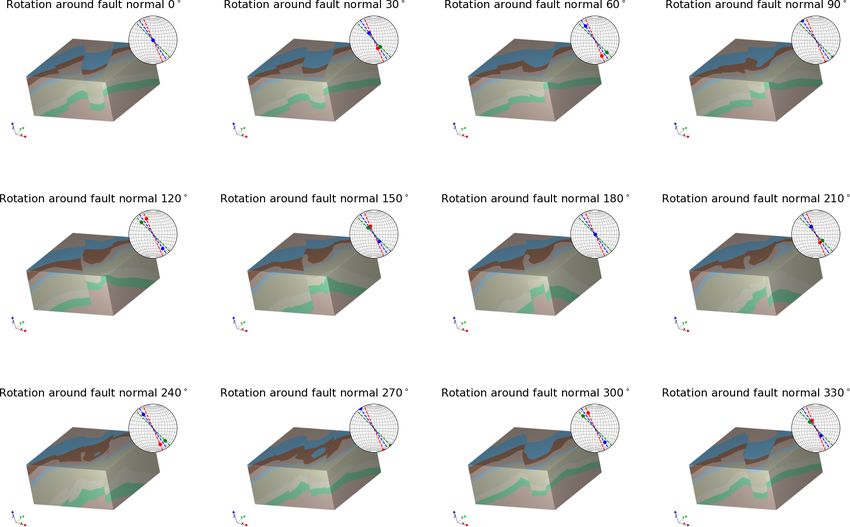
3916                                                    L. Grose et al.: LoopStructural 1.0: time-aware geological modelling

(2) discrete interpolation where the basis functions are lo-          This paper begins with a background analysis of 3D mod-
cated on a predefined support (Caumon et al., 2013; Frank et       elling methods and the algorithms used in implicit modelling,
al., 2007; Irakarama et al., 2018; Renaudeau et al., 2019).        with an overview of the mathematical and geological back-
The algorithms are often linked to commercial software,            grounds used in our implementation. A detailed overview of
e.g. Leapfrog1 , 3D GeoModeller2 and Gocad-SKUA3 . These           the specifics of the implementation can be found on (http://
packages will usually only provide one algorithm for interpo-      loop3d.github.io/LoopStructural, last access: 15 June 2021).
lation, making it difficult to compare different interpolation     To demonstrate the versatility of LoopStructural and to pro-
schemes. The algorithms are also usually black box algo-           vide a user guide we include four case studies in this paper
rithms with limited ability to change algorithm parameters,        with corresponding Jupyter notebooks. The first case study is
with no understanding of how the algorithm is implemented.         a synthetic example interpolating two planar surfaces where
A recent open-source Python library, Gempy (de la Varga et         the height of one surface has been perturbed to simulate un-
al., 2019), implements the dual co-kriging implicit interpo-       certainty in the surface location. In this example we use the
lation algorithm (Lajaunie et al., 1997) using a high perfor-      LoopStructural API to compare three different interpolation
mance computational library.                                       codes and investigate the parameters and how they are af-
   In this contribution we introduce the open-source Loop-         fected by noise. The second example is a synthetic refolded
Structural, a 3D geological modelling Python library based         type 3 interference pattern from Laurent et al. (2016), where
on the incremental contributions of Laurent et al. (2016) and      we apply the time-aware discrete fold interpolation method
Grose et al. (2017, 2018, 2019). LoopStructural is a new geo-      described by Laurent et al. (2016) for modelling the refolded
logical modelling engine developed within the Loop4 consor-        folds. In the third case study LoopStructural is applied to
tium (Ailleres et al., 2018). The core modelling library within    a real dataset from the Flinders Ranges in South Australia,
LoopStructural depends on scipy (Virtanen et al., 2020),           where the dataset has been prepared using the pre-processing
numpy (Van Der Walt et al., 2011) and pandas (pandas de-           module of the Loop workflow map2loop (Jessell et al., 2021).
velopment team, 2020), the core scientific Python libraries.       In the fourth and final case study we use map2loop to aug-
A visualisation module uses LavaVu (Kaluza et al., 2020),          ment an input dataset for a model in the Hamersley region in
a minimal OpenGL visualisation package allowing for mod-           Western Australia. We generate 10 unique models, demon-
els to be visualised within a Jupyter notebook environment.        strating the range of possible geometries when perturbing the
LoopStructural has been written using an object-oriented           fault geometry.
program design with class structures designed to allow for
powerful inheritance and modularity. The design of Loop-
Structural allows development and research into geological         2    Materials and methods
modelling methods to be easily performed without having to
rewrite boiler plate code for interpolation algorithms, visual-    A 3D geological model can be represented by a collection of
isation and model interaction. LoopStructural is a modelling       surfaces representing geological features (e.g. fault surfaces,
package allowing for multiple stratigraphic groups, faults,        stratigraphic horizons, axial surfaces of folds, unconformi-
folds and unconformities to be represented using implicit sur-     ties) (Wellmann and Caumon, 2018). There are two main
faces. Different interpolation algorithms can be used for in-      tasks for a 3D modelling software package:
terpolating these surfaces with the ability to mix and match
                                                                       – the creation of the surfaces from geological observa-
interpolation algorithms depending on the surface type be-
                                                                         tions and knowledge, this is known as interpolation;
ing modelled. LoopStructural has native implementation of
discrete implicit modelling using a piecewise linear interpo-          – the incorporation of geological concepts into the surface
lation on a tetrahedral mesh (Caumon et al., 2013; Frank et              description, e.g. faulted surfaces should show displace-
al., 2007; Mallet, 2014, 2002), finite-difference interpolation          ment and unconformities should be a boundary between
on a Cartesian grid (Irakarama et al., 2018; Renaudeau et al.,           units.
2018), fold interpolation using tetrahedral meshes (Laurent
et al., 2016) and an interface to a generalised radial basis in-   In LoopStructural surfaces are implicitly represented by an
terpolation (Hillier et al., 2014).                                isovalue of one or more volumetric scalar fields (Calcagno et
                                                                   al., 2008a; Caumon et al., 2013; Cowan et al., 2003; Frank et
                                                                   al., 2007; Gonçalves et al., 2017; Hillier et al., 2014; Jessell,
   1 https://www.seequent.com/products-solutions/                  1981; de la Varga et al., 2019; Lajaunie et al., 1997; Mal-
leapfrog-software/; last access: 15 June 2021                      let, 2002, 2014; Manchuk and Deutsch, 2019; Maxelon et al.,
    2 https://www.intrepid-geophysics.com/product/geomodeller/;    2009; Moyen et al., 2004; Renaudeau et al., 2019; Yang et al.,
last access: 15 June 2021                                          2019). The geological rules are managed by adding the geo-
    3 https://www.pdgm.com/products/skua-gocad/; last access:      logical event (folding event, one fault, another fault, an un-
15 June 2021                                                       conformity) structural parameters in a time-aware approach,
    4 https://www.loop3d.org; last access: 15 June 2021            where the most recent event is added first and the constraints

Geosci. Model Dev., 14, 3915–3937, 2021                                             https://doi.org/10.5194/gmd-14-3915-2021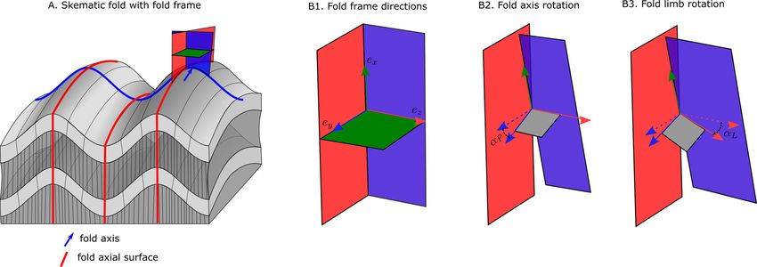
L. Grose et al.: LoopStructural 1.0: time-aware geological modelling                                                         3917

are added backwards in time. Complex geological features           2.1.1     Input data
such as folds and faults are integrated into LoopStructural by
building a structural frame around the principal structural di-    Geological observations that are directly incorporated into
rections of the feature being modelled. Using these structural     3D modelling can generally be divided into two categories:
frames geological rules can be integrated into the modelling       observations that describe the orientation of a geological fea-
workflows – e.g. fault kinematics can be added to the faulted      ture (on contact and off contact) and observations that de-
feature because the fault geometry is known before interpo-        scribe the location within a geological feature (cumulative
lating the faulted feature or fold overprinting relationships      thickness for conformable stratigraphic horizons, or location
can be incorporated using multiple structural frames (Lau-         of fault surface). In the context of a geological map, location
rent et al., 2016).                                                observations may be the trace of a geological surface on the
                                                                   geological map, or a single point observation at an outcrop or
2.1   Implicit surface modelling                                   from a borehole. Orientation observations generally record a
                                                                   geometrical property of the surface – e.g. a vector that is tan-
Implicit surface modelling involves the representation of the      gential to the plane or the vector that is normal to the plane
geometry of a geological feature using a function f (xyz)          (black and dashed arrows in Fig. 1).
where the value of the function is the same along the obser-          When modelling using the potential field approach, the
vation of the surface. There are two possible ways of framing      value of the scalar field is inferred through the magnitude
this question. The first approach uses the scalar field value as   of the normal control points. Using the signed distance ap-
a distance from a reference horizon, e.g. the location of the      proach, the value of the scalar field is defined by the value of
horizon for a single surface would be the value of the scalar      the observations and effectively controls the thickness of the
field. Using this approach, which we will call the signed dis-     layers. Orientation constraints either control a component of
tance approach, the same implicit function can represent con-      the orientation, e.g. specifying that the gradient of the func-
formable horizons where the value of each horizon is the cu-       tion should be orthogonal to the observation or constrain the
mulative thickness from the base of the series (Caumon et          magnitude and direction of the norm of the gradient of the
al., 2013; Hillier et al., 2014; Jessell, 1981; Manchuk and        implicit function.
Deutsch, 2019; Wellmann and Caumon, 2018). The second                 All geological observations constrain a component of the
approach, often referred to as the potential field approach,       implicit function at a location in the model:
does not specify the value of the scalar field. The potential
field approach only defines the potential field to have the          – Observations for the location of the geological feature
same value for specific interfaces, such as contacts between           will constrain the value of the scalar field f (x, y, z) =
geological units and fault traces (Calcagno et al., 2008a; de          v.
la Varga et al., 2019). As with the signed distance field, the
potential field can represent conformable horizons – where           – Observations for the orientation of the contact can either
the value of the implicit function evaluated on the input ob-
servations can be used to infer the potential field value for
these horizons.                                                            • constrain the partial derivatives of the function
   These implicit functions have no known analytical solu-                     ∇f (x, y, z) = n or
tion, which means that they need to be approximated from
                                                                           • constrain a vector which is parallel to the contact
the observations that are provided. The implicit function is
                                                                               ∇f (x, y, z) · t = 0.
represented by a weighted combination of basis functions:

            N
            X                                                      It is worth noting that when constraining the partial deriva-
f (xyz) =         wi · ϕi (x, y, z),                        (1)    tive of the scalar field, the norm of the vector defines the
            i=0                                                    norm of the implicit function which controls the distance be-
                                                                   tween isosurfaces. The sign of the vector must be consistent
where N is the number of basis functions, w are the weights        with the polarity of the structural observation, e.g. for bed-
and ϕ are the basis functions. There are two approaches for        ding this must be the younging direction. Structural orien-
approximating the implicit function: the first approach uses       tations can also be incorporated into the model using two
a discrete formulation for the interpolation where N is de-        tangent constraints where t 1 × t 2 = n, where × is the vector
fined by some sort of mesh (Caumon et al., 2013; Frank et          product. In the following sections we will outline the the-
al., 2007; Mallet, 1992; Moyen et al., 2004), and the second       oretical background for the piecewise linear interpolation,
approach uses data-supported basis functions where N is de-        finite-difference interpolation and data-supported interpola-
fined by the number of data points (Calcagno et al., 2008a;        tion. Within all approaches, the observations are incorporated
Cowan et al., 2003; Gonçalves et al., 2017; Hillier et al.,        by adding observations as constraints into a linear system of
2014; de la Varga et al., 2019; Lajaunie et al., 1997).            equations.

https://doi.org/10.5194/gmd-14-3915-2021                                               Geosci. Model Dev., 14, 3915–3937, 2021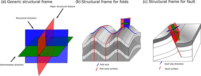
3918                                                         L. Grose et al.: LoopStructural 1.0: time-aware geological modelling

Figure 1. Schematic showing different types of interpolation constraints that can be applied to an implicit interpolation scheme in 2-D. There
are two interfaces: the reference horizon with a value of 0 and the next interface with a value of 1. Here we show three types of constraints:
(1) scalar field norm constraints constrain the orientation of the scalar field and the norm of the implicit function at that location; (2) scalar
field value constraints control the value of the scalar field; and (3) tangent constraints constrain only the orientation of the implicit function
not the norm. Figure adapted from Hillier et al. (2014).

2.1.2   Piece-wise linear interpolation                                    of the point within the cell. Different regularisation terms can
                                                                           be used; for example Irakarama et al. (2018) minimise the
The volumetric scalar field is defined by a piece-wise lin-                sum of the second derivatives:
ear function on a volumetric tetrahedral mesh. In LoopStruc-
tural the volumetric tetrahedral mesh creation is simplified                ∂2   ∂2   ∂2    ∂2     ∂2     ∂2
                                                                               +    +    +2     +2     +2     = 0.                            (3)
by subdividing a regular Cartesian grid into a tetrahedral                  ∂xx ∂yy ∂zz     ∂xy    ∂yz    ∂zx
mesh where one cubic element is divided into five tetrahe-
dra (see Appendix A). The linear tetrahedron is the basis of               Alternatively, a partial differential equation such as the bend-
the piecewise linear interpolation algorithm, where the prop-              ing energy (Renaudeau et al., 2019) or Gaussian curvature
erty within the tetrahedron is interpolated using a linear func-           could be used. In LoopStructural 1.0, currently only the sum
tion; see Appendix A for a detailed description of the linear              of the second derivatives can be used. The object-oriented
basis function. We use constant gradient regularisation (Cau-              program design would allow for different regularisation con-
mon et al., 2013; Frank et al., 2007; Mallet, 1992), where                 straints to be implemented without requiring any boiler plate
the change in gradient of the implicit function is minimised               code.
between tetrahedra with a shared face. The constant gradient
regularisation is as follows:                                              2.1.4    Solving discrete interpolation

∇ϕ T1 · n − ∇ϕ T2 · n = 0,                                        (2)      Using either the piecewise linear interpolator or the finite-
                                                                           difference interpolator the scalar field is defined by the node
where ∂ϕ T1 is the gradient of the first tetrahedron, ∂ϕ T2 is             values of the support. These can be found by solving a system
the gradient of the second tetrahedron and n is the normal                 of equations with M unknowns x1 , . . ., xM (Caumon et al.,
vector to the shared face.                                                 2013; Frank et al., 2007; Mallet, 2004). The unknowns can
                                                                           be found by solving the linear system of equations:
2.1.3   Finite-difference interpolation
                                                                           A · x = b,                                                         (4)
The second discrete interpolation approach approximates the
interpolant using a combination of tri-linear basis functions              where A is an N ×M sparse matrix containing the linear con-
on a Cartesian grid. The basis functions describe the interpo-             straints and b the right-hand side vector containing the obser-
lation as a function of the corners of the cell within which               vation of constraint value. For example, to integrate value
the point where the function is to be estimated falls; see Ap-             observations the row in the interpolation matrix A would
pendix B for the trilinear basis functions. For example, to                contain the shape parameters for the cell in which the point
evaluate the value of the implicit function at a point xi yi zi ,          is contained. The right-hand side would be the value of the
first the cell c is found using integer division of the point              scalar field.
coordinates and the grid step vector, where the integer corre-                The interpolation problem is over-constrained, i.e. N >
sponds to the index of the cell in the grid. The local coordi-             M, and can be solved in a least squares sense. The least
nates (ξ , η, ζ ) are determined by finding the relative location          squares problem can be solved using a number of different

Geosci. Model Dev., 14, 3915–3937, 2021                                                       https://doi.org/10.5194/gmd-14-3915-2021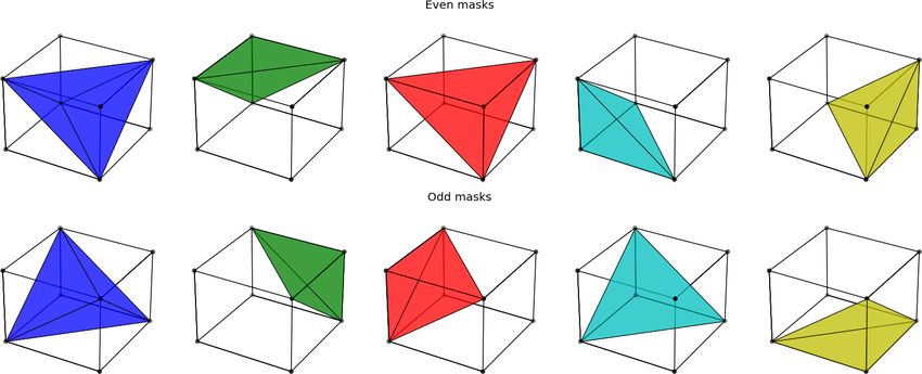
L. Grose et al.: LoopStructural 1.0: time-aware geological modelling                                                          3919

algorithms either directly where AT · A is directly inverted,       These geological interfaces can all be affected by deforma-
e.g. using lower–upper decomposition, or using an iterative         tional structures such as folds, faults and shear zones. In the
algorithm such as conjugate gradient. Generally, for large          following sections we will describe how these different geo-
problems an iterative approach is recommended because it            logical features are integrated into 3D modelling workflows
requires less memory. LoopStructural allows for multiple            by describing how different scalar fields interact and how the
different solvers to be used for the least squares problem.         structural geology of faults and folds are added into the im-
The default solver is the conjugate gradient algorithm imple-       plicit surface description.
mented in scipy. To speed up the solver and in some cases
improve the stability of the solution we provide the option of      2.2.1   Stratigraphic contacts
adding a small value (the smallest representable float) to the
diagonal of the square matrix (AT · A).                             In an implicit geological model, the distribution of strati-
                                                                    graphic packages is defined by the values of a volumetric
2.1.5    Data-supported interpolation                               scalar field. The scalar field is defined by an implicit func-
                                                                    tion that is fitted to observations (location and orientation)
Another approach for implicit surface modelling is to use           defining the geometry of the top or base of a geological unit.
basis functions that are located at the same location as data       A single geological interface can be modelled using a sin-
points.                                                             gle scalar field, or multiple conformable interfaces can be
   This can be done using radial basis interpolation where          modelled using a single scalar field where different isovalues
the interpolation problem is attempting to approximate the          are used to represent the different contacts. A stratigraphic
signed distance field:                                              group can be considered as a collection of stratigraphic sur-
                N
                X                                                   faces that are conformable. When modelling a stratigraphic
f (x, y, z) =         wi · ϕ (X) + P (x, y, z).              (5)    group, the value of the scalar field represents the distance
                i=0                                                 away from the base of a group of conformable layers.
                                                                       An unconformity is a geological interface where the rock
Alternatively, the problem can be represented using dual co-
                                                                    units on either side are of significantly different ages, usu-
kriging (Calcagno et al., 2008b; de la Varga et al., 2019; La-
                                                                    ally representing a period of erosion. In Fig. 3 the three con-
jaunie et al., 1997), where the interpolation algorithm esti-
                                                                    ventional types of unconformity are shown. In Fig. 3a. the
mates the potential field, which estimates incremental differ-
                                                                    unconformity between the units is a disconformity and the
ences between the scalar field for different horizons. Using
                                                                    geometry of the disconformity is not associated with either
this approach, the system is separated into two parts: (1) the
                                                                    stratigraphic package. The disconformity is usually identi-
orientation observations which are incorporated using the di-
                                                                    fied by the significant gap between the ages of the rocks. In
rection and magnitude and (2) the difference between the po-
                                                                    this type of contact the layers actually share a similar ge-
tential field for different horizons.
                                                                    ometry and for the purpose of 3D modelling the units could
   LoopStructural uses SurfE, a C++ implementation of the
                                                                    be represented by a single stratigraphic group. Angular un-
generalised radial basis interpolation (Hillier et al., 2014) for
                                                                    conformities (Fig. 3b) are observed when erosion occurs af-
all data-supported interpolations. SurfE has three approaches
                                                                    ter some deformation (the older beds are not horizontal any-
for implicit surface reconstruction (1) signed distance inter-
                                                                    more) and before the next deposition of sedimentary layers.
polation using radial basis functions, (2) potential field in-
                                                                    As the name suggests the angular unconformity represents a
terpolation using dual co-kriging (Lajaunie et al., 1997) and
                                                                    boundary between two differently oriented stratigraphic se-
(3) signed distance interpolation using a separate scalar field
                                                                    quences. In a 3D model an angular unconformity can be in-
for each surface. The interface between LoopStructural and
                                                                    troduced by setting the boundary between the two sequences
SurfE allows the user to access all of the interpolation pa-
                                                                    to be the base of the younger package. In practice, this means
rameters used by SurfE. These include access to more so-
                                                                    that the two groups are modelled with two separate scalar
phisticated solvers, as well as the addition of a smoothing
                                                                    fields. In Fig. 3c a nonconformity is shown; in this type of
parameter into the interpolation.
                                                                    unconformity the geometry of the older unit defines the base
2.2     Modelling geological features                               of the younger unit. This could occur when a stratigraphic
                                                                    package is deposited on top of a crystalline basement.
There are three ways that the geometry of rock packages can
structurally interact in a geological model:                        2.2.2   Structural frames

  1. stratigraphic contacts – the contact between sedimen-          A structural frame (Fig. 4) is a local coordinate system that
     tary layers;                                                   is built around the major structural elements of a geological
  2. fault contacts;                                                event. In LoopStructural structural frames are used for char-
                                                                    acterising the geometry of folds where the major structural
  3. intrusive contacts.                                            element is the fold axial foliation (Fig. 4b) and the structural

https://doi.org/10.5194/gmd-14-3915-2021                                              Geosci. Model Dev., 14, 3915–3937, 2021
3920                                                       L. Grose et al.: LoopStructural 1.0: time-aware geological modelling

Figure 2. Unconformities interfaces (red lines) and geological interfaces (black lines) represent a break in depositional history. There are
different possible geometries that an unconformity can have: (a) disconformity contact between two stratigraphic packages that share a
similar geometry, (b) an angular unconformity where the younger stratigraphic package defines the geometry of the unconformity and (c) a
nonconformity where the older stratigraphic package defines the geometry of the unconformity.

direction is roughly the fold axis. A fault frame is a structural       the surfaces displaced by the fault. The fault surface can be
frame where the major structural feature is the fault surface,          interpolated by building a scalar field where the fault surface
the structural direction is the fault slip and the intermedi-           is represented by an isovalue.
ate direction is the fault extent (Fig. 4). In LoopStructural,             In LoopStructural there are two ways of representing
structural frames are built by first building the major struc-          faults: (1) the fault kinematics are added into the implicit de-
tural feature which will typically have more observations,              scription of the scalar field of the faults and applied to the
e.g. fault surface location or axial foliations. The structural         affected scalar field(s) (Grose et al., 2021a) and (2) faults
direction is then built using any available observations of the         are treated as domain boundaries and separate scalar fields
structural direction, e.g. local observations of the fault slip or      are used to model the hanging wall and footwall of the fault.
the fold axis, combined with an additional constraint which             The kinematics of the fault are added into the implicit de-
sets the gradient of the scalar field to be orthogonal to the ma-       scription of the faulted surface. To do this a fault frame is
jor structural feature. The third coordinate can be built with          built (Fig. 4c) where three coordinates are interpolated: (1) a
an arbitrary value constraint, or value constraints to specify          scalar field representing the distance to the fault surface, (2) a
the extent of the field in this direction (e.g. for faults −1 and 1     scalar field representing the distance along the slip direction
specify the edges of the fault). This value constraint is com-          of the fault and (3) a scalar field representing the extent of the
bined with two global orthogonality constraints specifying              fault. These coordinates can then be used to define the fault
that the scalar field should be orthogonal to both the major            ellipsoid, which is a volumetric representation of the area de-
structural feature and the structural direction.                        formed by the fault. The displacement of the fault can be de-
                                                                        fined relative to this coordinate system, e.g. the displacement
2.2.3   Faults                                                          of the fault should decay away from the fault centre along
                                                                        the fault extent and along the direction of displacement us-
“A fault is a tabular volume of rock consisting of a central            ing the bell-shaped curve (Fig. 5d). The displacement may
slip surface or core, formed by an intense shearing, and a              decrease with distance away from the fault centre perpendic-
surrounding volume of rock that has been affected by more               ular to the fault surface; this can be defined using the profile
gentle brittle deformation spatially and genetically related to         in Fig. 5c. If the displacement is constant within the model
the fault” (Fossen, 2010).                                              area the curves in Fig. 5a and b can be substituted for Fig. 5c
   When adding faults there are two aspects to modelling the            and d respectively. The displacement curves shown in Fig. 5
fault: (1) building the fault surface geometry and (2) integrat-        can be substituted for any function of the fault frame coor-
ing the fault displacement into older surfaces. Where possi-            dinates. The same approach for combining the fault profiles
ble, measurements of faults include the movement direction              (Fig. 5) within the fault frame has been used to define a vol-
and the magnitude of displacement. There are three broad                umetric fault displacement field (Jessell and Valenta, 1996;
approaches for integrating faults into the implicit modelling           Godefroy et al., 2018b), the latter of which was adapted from
framework: (1) add the fault into the implicit description of           the following Laurent et al. (2013):
the surface (Calcagno et al., 2008a; de la Varga et al., 2019);

(2) apply the fault after interpolating a continuous surface            δ (x) = D0 f0(X) · D1 (f1 (X)) · D2 (f2 (X)) ,                 (6)
(Godefroy et al., 2018a; Laurent et al., 2013) and (3) rep-
resent the foot wall and hanging wall by separate implicit              where D0,1,2 are 1-D curves (e.g. any of the curves in Fig. 5)
functions. Regardless of the approach used, the geometry of             describing the displacement of the fault within the fault
the fault surface is defined before defining the geometry of            frame.

Geosci. Model Dev., 14, 3915–3937, 2021                                                   https://doi.org/10.5194/gmd-14-3915-2021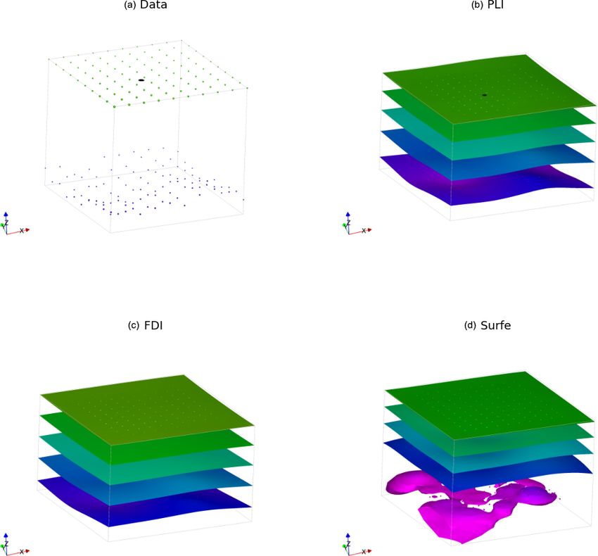
L. Grose et al.: LoopStructural 1.0: time-aware geological modelling                                                                      3921

Figure 3. (a) Generic structural frame showing isosurfaces for three coordinates. (b) Structural frame for characterising a fold. (c) Structural
frame for characterising fault geometry.

Figure 4. Fault displacement profiles: (a) constant displacement profile, (b) infinite-extent fault displacement showing no change in fault
displacement along the fault extent or in the slip direction, (c) finite-extent fault displacement showing fault displacement decreasing with
distance away from the fault, (d) finite-extent fault bell shaped profile for characterising fault displacement along the fault extent or in the
slip direction.

   The fault frame can be built using a discrete implicit mod-            trace and fault slip direction are known, the fault can be mod-
elling approach as additional constraints can be added into               elled. Where the fault slip is unknown, this can be substituted
the interpolation to enforce the orthogonality of the three co-           by conceptual knowledge, e.g. enforcing strike-slip faults or
ordinate systems. This is added into the interpolation matrix             reverse faults.
by adding a constraint for every element in the mesh where
∇φ0 (x, y, z)·∇φ1 (x, y, z) = 0. This constraint can be added             2.2.4    Folds
twice so that when modelling φ2 both φ0 and φ1 are orthog-
onal. In general, this means that if the fault orientation, fault         Folds are challenging to model using classical implicit inter-
                                                                          polation algorithms, because by definition a folded surface

https://doi.org/10.5194/gmd-14-3915-2021                                                       Geosci. Model Dev., 14, 3915–3937, 2021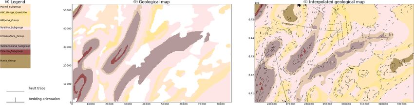
3922                                                     L. Grose et al.: LoopStructural 1.0: time-aware geological modelling

has a symmetry only defined by their axial surface. The sym-        The fold constraints require two angles to be known through-
metry is hard to reproduce by only interpolating orientations       out the model: the fold axis rotation angle (αP ) and the fold
of the folded foliation as this would require orientations to       limb rotation angle (αL ). The fold axis rotation angle (αP ) is
be sampled in a symmetrical way across the axial surface            the angle between the fold axis and ey (Grose et al., 2017).
(Laurent et al., 2016; Lisle et al., 2007; Mynatt et al., 2007).       The fold limb rotation angle (αL ) is the angle that defines
The regularisation of implicit algorithms are usually defined       the orientation of the folded foliation relative to fold axial fo-
to minimise some sort of curvature between observations             liation and will be 0 in the hinge of the fold and positive and
such as constant gradient regularisation, minimising second         negative in the limbs (Grose et al., 2017). Grose et al. (2017)
derivatives using finite differences or the weighted combi-         used the fold frame to calculate these angles for observations
nation of infinite basis functions (Calcagno et al., 2008a;         and then applied interpolation either using radial basis func-
Cowan et al., 2003; Frank et al., 2007; Jessell et al., 2014; La-   tions or by fitting an objective function (a Fourier series) to
jaunie et al., 1997; Laurent, 2016; Mallet, 2014). As a result,     the rotation angles within the fold frame coordinates. The
to model folded geometries the geologist is required to add         wavelength of the fold can be estimated by calculating an
interpretive constraints such as synthetic bore holes, cross        experimental semi-variogram of the fold rotation angle in
sections or simply synthetic constraints to produce model ge-       the fold frame coordinates. For periodic folding, the exper-
ometries that fit the geologist’s conceptual idea of the fold       imental variogram has a periodic curve where the first peak
(Caumon et al., 2003; Jessell et al., 2014, 2010).                  indicates the half-wavelength of the fold (Grose et al., 2017).
   There have been a number of different approaches to in-             In LoopStructural the default approach for fitting the fold
corporating folds into implicit modelling including incorpo-        rotation angle is to fit a Fourier series. The fold axis rota-
rating the fold axial surfaces (Laurent et al., 2016; Maxelon       tion angle is calculated first; the wavelength is first estimated
et al., 2009), the fold axis (Hillier et al., 2014; Laurent et      automatically using the gradient descent method on the ex-
al., 2016; Massiot and Caumon, 2010), both these structural         perimental variogram of the fold axis. The fold rotation an-
elements and fold overprinting relationships (Laurent et al.,       gle is optimised using the scipy.optimize.curve_fit method
2016).                                                              using non-linear least squares to fit wavelength and Fourier
   LoopStructural implements the following fold constraints:        coefficients. The fold axis can then be defined throughout the
the fold axis, fold axial surface and overprinting relationships    model by applying the rotation of ey · Rp . If the fold axis is
(Laurent et al., 2016) by adding additional constraints into a      constant (cylindrical folding), a constant fold axis vector can
discrete interpolation approach. A fold frame (Figs. 4b and 6)      be used.
is built where the principal axes of the fold frame correspond         The fold limb rotation angle is calculated by finding the
with the direction of the finite-strain ellipsoid. The fold frame   complementary angle between the normal to the folded fo-
allows for the geometry of the folded surface to be defined.        liation and ez in the plane perpendicular to the fold axis.
   The orientation of the fold axis (FTA ) can be defined within    The fold limb rotation angle can be interpolated by fitting
the fold frame by rotating the fold axis direction field by the     a Fourier series to the observations in the same way as fitting
fold axis rotation angle (Fig. 6b2). The fold direction (FTD ) is   the fold axis rotation angle.
defined by rotating the normal to the axial foliation around           Grose et al. (2018, 2019) use inverse problem theory to fit
the fold axis by the fold limb rotation angle. The orienta-         a forward model of the fold geometry to the observed fold
tion of the folded surface is the plane defined by the fold         rotation angles. The joint posterior distribution of the fold
axis vector and the fold direction vector (Fig. 6b3). The fold      parameters (Fourier series coefficients, fold wavelength and
constraints have been implemented into the piecewise linear         a misfit parameter) are sampled using Bayesian inference.
interpolator using four main constraints, where ϕ(xyz) rep-         This allows multiple fold geometries to be explored without
resents the implicit function, ∇ represents the gradient, t rep-    perturbing the datasets. LoopStructural does not provide a di-
resents a tetrahedron where the constraint is applied and T1        rect probabilistic interface; however, it is possible to define a
and T2 are two tetrahedrons that share a face, and hs is the        probabilistic representation of the fold geometry curves and
expected magnitude of the gradient norm:                            add this into the modelling workflow. An example using the
  – The folded surface should contain the orientation of the        Python library emcee (Foreman-Mackey et al., 2013) is pro-
    fold axis: FTA · ∇ϕ(xyz) = 0.                                   vided in the LoopStructural documentation.

  – The folded surface will contain the fold direction (solid
    red arrow in Fig. 6b3) vector: FTD · ∇ϕ(xyz) = 0.               3     Implementation in LoopStructural
  – The regularisation should only occur within the inter-
    mediate structural direction (ex ) etx0 · ∇ϕT1 (xyz) − etx1 ·   3.1    Loop structural design
    ∇ϕT2 (xyz) = 0.
                                                                    LoopStructural is written using Python 3.6+, using numpy
  – A similar fold constraint is as follows: etx · ∇ϕ(xyz) =        data structures and operations. The design of LoopStructural
    1
    hs .                                                            follows an object-oriented architecture with multiple levels

Geosci. Model Dev., 14, 3915–3937, 2021                                              https://doi.org/10.5194/gmd-14-3915-2021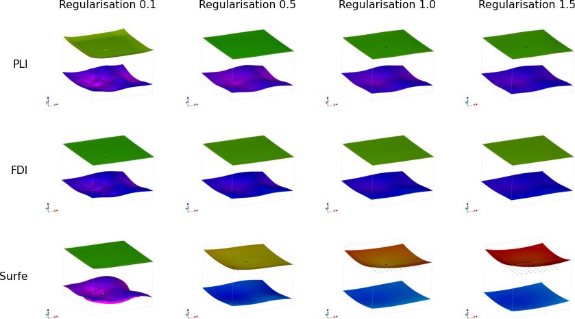
L. Grose et al.: LoopStructural 1.0: time-aware geological modelling                                                                   3923

Figure 5. Schematic diagram of a fold adapted from Laurent et al. (2016) showing (a) fold frame, (b1) fold frame direction vectors, (b2) fold
axis defined by fold axis rotation angle, (b3) folded foliation defined by fold limb rotation around fold axis.

of inheritance. Object-oriented design allows for LoopStruc-               3. tangent is the scalar field and should be orthogonal to a
tural to be used as a development platform for 3D geological                  vector.
modelling, where new features can be added without needing
to implement boiler plate code. There are five submodules                  4. norm constrains the direction and magnitude of the
that can be imported into a Python environment:                               scalar field norm.

  1. core contains the core modelling functionalities and the            The data can be associated with the GeologicalModel us-
     management of the geological concepts.                              ing the set_data(data) method where “data” is a pandas data
                                                                         frame. When added into the model the data points are trans-
  2. interpolation contains the various interpolation code               formed into the model coordinate system.
     and supports used to build scalar fields.
                                                                         3.2   Adding geological objects
  3. datasets contains the test and reference datasets.
                                                                         Within LoopStructural geological objects such as stratigra-
  4. utils contains miscellaneous functions.                             phy, faults, folding event and unconformities are all repre-
  5. visualisation contains model visualisation tools.                   sented by a GeologicalFeature. A GeologicalFeature can be
                                                                         evaluated for the value of the scalar field and/or the gradient
The creation and management of different geological ob-                  of the scalar field at a location.
jects is managed by the GeologicalModel. To initialise an                   The GeologicalModel contains an ordered collection of
instance, the required arguments are the minimum and maxi-               geological features and determines how the features interact.
mum extents of the bounding box, which are specified by two              For example, unconformity geological features act as a mask
separate vectors. The default behaviour is to define a rescal-           to determine where the interface between packages should
ing coefficient as follows:                                              be. The ordering of the GeologicalFeatures inside the model
                                                                         reflects the timing of the geological events being modelled.
scale = max(xmax − xmin , ymax − ymin zmax − zmin ).            (7)      The most recent features are added first as their geometry is
                                                                         used to constrain the older features.
Adding different geological objects can be done through us-                 There are different ways a GeologicalFeature can be added
ing an instance of GeologicalModel. There are four different             to a GeologicalModel depending on the type of geological
types of observations that can be incorporated into an inter-            object that is being modelled. The LoopStructural Geologi-
polation algorithm:                                                      calModel class provides an interface for creating geological
  1. value constrains the value of the scalar field at a partic-         objects, where different types of geological features can be
     ular location and can either represent the location of a            added using different functions. All geological objects are
     surface or the distance away from the surface.                      represented by one or multiple volumetric scalar field. These
                                                                         scalar fields can be built using an implicit interpolation algo-
  2. gradient constrains only the gradient of the scalar field;          rithm where the implicit function is approximated from ob-
     e.g. the normal to the scalar field should be orthogonal            servations of the scalar field. Alternatively, a GeologicalFea-
     to two vectors within the gradient plane.                           ture can be represented by an analytical function (or a com-

https://doi.org/10.5194/gmd-14-3915-2021                                                     Geosci. Model Dev., 14, 3915–3937, 2021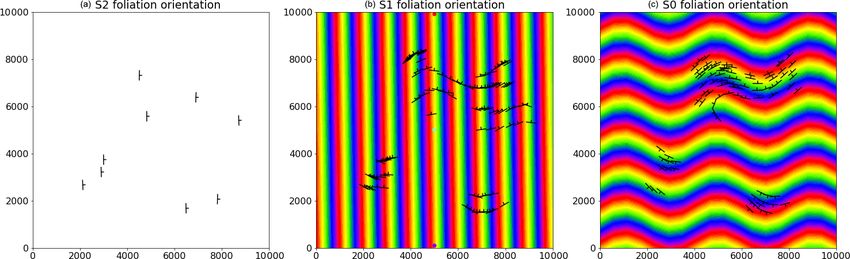
3924                                                        L. Grose et al.: LoopStructural 1.0: time-aware geological modelling

Figure 6. Comparison of interpolation methods for synthetic surfaces where two isosurfaces are shown coloured by the local z coordinate:
(a) input data, (b) surfaces interpolated using PLI, (c) surfaces interpolated using FDI, (d) surfaces interpolated using SurfE; note the lower
isosurface has a non-manifold geometry.

bination of existing GeologicalFeatures). LoopStructural al-              within the model. The following functions can be called from
lows for different interpolation algorithms to be specified for           a GeologicalModel as shown in the code below.
different GeologicalFeatures within the same model. The in-
terpolation algorithm and any parameter definitions are spec-                – To evaluate the lithology value at a location the function
ified by adding additional keyword arguments to the func-                      evaluate_model(xyz) returns a numpy array containing
tion. Table 1 outlines the possible arguments that can be spec-                the integer ID of the stratigraphy that was specified in
ified for the interpolator.                                                    the stratigraphic column.

3.3    Model output                                                          – To evaluate the value of a GeologicalFeature at
                                                                               a location within the model the function evalu-
LoopStructural includes a number of helper functions for                       ate_feature_value(feature_name,xyz) returns the value
evaluating the GeologicalModel on an array of coordinates                      of the scalar field that represents the geological feature.

Geosci. Model Dev., 14, 3915–3937, 2021                                                     https://doi.org/10.5194/gmd-14-3915-2021
L. Grose et al.: LoopStructural 1.0: time-aware geological modelling 3925
Table 1. Interpolation keyword arguments. Default values are highlighted by bold text.
Keyword arguments Description Possible values
Interpolator_type A choice for what interpolator to use “PLI”, “FDI”, “Surfe”, “DFI”
solver Which algorithm to solve the least squares “cg”, “lu”, “pyamg”, “lsqr”, “lsmr”, “custom”
problem (for PLI, FDI and DFI)
nelements Number of elements in the discrete interpola- 100 : ∞, 100 000
tion approach
buffer How much bigger to mesh around the model ex- 0 : ∞, 0.2
tents
cpw Weighting of value constraints in discrete least 0 : ∞, 1
squares problem
gpw Weighting of gradient constraints in discrete 0 : ∞, 1
least squares problem
npw Weighting of norm constraints in discrete least 0 : ∞, 1
squares problem
tpw Weighting of tangent constraints in discrete 0 : ∞, 1
least squares problem
regularisation Weighting of regularisation constraints in least 0 : ∞, 1
squares problem
data_region Buffer around the observations to interpolate Boolean function, None
scalar field only on a subsection of the mesh
– To evaluate the gradient of a GeologicalFeature the eval- geological map from the resulting geological model. In-
uate_feature_gradient(feature_name,xyz) can be called. put datasets can be plotted drawing the location of con-
tacts and the orientation of the contacts using the strike
Triangulated surfaces can be extracted from a Geologi- and dip symbology. The scalar field can be evaluated on
calFeature within LoopStructural and exported into common the map surface, contours can be drawn or the geologi-
mesh formats, e.g. Visualisation ToolKit (.vtk) or Wavefront cal model can be plotted onto the map.
(.obj). These surfaces can then be imported into external soft-
ware, e.g. ParaView5 . 3. FoldRotationAnglePlotter. This is a visualisation mod-
ule for producing S plots and S-variogram plots for a
3.4 Model visualisation folded geological feature. Plotting is handled using mat-
plotlib.
LoopStructural has three different visualisation tools that can
be accessed from the LoopStructural.visualisation module:
4 Examples
1. LavaVuModelViewer. LavaVu (Kaluza et al., 2020) is
a visualisation module that provides interactive visuali- 4.1 Implicit surface modelling
sation. We use LavaVu for visualising triangulated sur-
faces representing the geological interfaces as well as In the first example we will demonstrate modelling two syn-
the scalar field representing the implicit function. The thetic surfaces using the same scalar field within a model vol-
creation and manipulation of LavaVu objects is wrapped ume of (−0.1, −0.1, −0.1) and (5.1, 5.1, 5.1). The observa-
by the LavaVuModelViewer class which provides an in- tions are two sets of points. The first set forms a surface at
terface to the GeologicalModel. This is an interactive points on a regular grid for z = 4 and the second set forms a
(and static) 3D visualisation using LavaVu. surface at z = 0.2·sin (x · 10)+0.2·cos (y)+0.15·N (0, 0.1)
where N (0, 0.1) is a normal distribution with a mean of 0
2. MapView. This is a 2D visualisation (cross section, and standard deviation of 0.1.
map) using matplotlib (Hunter, 2007) that can create a In Fig. 7a the data points are shown, and in Fig. 7b, c and
d the same surfaces are interpolated using the three default
5 https://www.paraview.org/, last access: 15 June 2021 interpolation algorithms in LoopStructural (PLI – piecewise
https://doi.org/10.5194/gmd-14-3915-2021 Geosci. Model Dev., 14, 3915–3937, 20213926 L. Grose et al.: LoopStructural 1.0: time-aware geological modelling
Figure 7. Implicit surfaces calculated for regularisation constraints (0.1,0.5,1,1.5) using piecewise linear interpolator (PLI), finite-difference
interpolator (FDI) and radial basis function (SurfE).
linear interpolator, FDI – finite-difference interpolator and a surface where the underlying process causing the varia-
SurfE – radial basis interpolation). The results for the inter- tion in the data points is non-stationary, a higher regulari-
polation using PLI and FDI are very similar, as both interpo- sation constraint is appealing as the goal of the modelling is
lation algorithms use least squares to fit observations whilst to reproduce the effect of this process. However, if the per-
minimising a global regularisation term that effectively min- turbations are the result of a process we are trying to model
imises the second derivative of the implicit function. This (probably a stationary process) then a lower regularisation
means that the interpolant balances fitting the observations constraint would be appealing. A smoothing constraint can
with minimising the roughness of the resulting surfaces. The be added into the radial basis interpolation which aims to in-
radial basis interpolation used by SurfE is a direct interpo- crease the smoothness of the resulting surface. The smooth-
lation approach, which means that the interpolant must fit ing constraint for data-supported methods adds a buffer to
all of the observations (although a smoothing constraint can how closely the function must fit the observations. In Fig. 8
be used). In this example, because the surfaces are over- increasing regularisation results in smoother surfaces; how-
constrained to a highly variable point set the resulting surface ever, with this approach the fit to both surfaces is impacted,
is non-manifold (cannot be unfolded into a flat plane). While which can be seen by the change in colour of the surface,
this does not necessarily mean the surface is incorrect it is which represents the local height of the surface.
geologically unlikely.
The weighting of the regularisation constraint generally 4.2 Modelling folds: type 3 interference
has the biggest impact on the resulting geometry when using
the discrete interpolation approaches. In Fig. 8 the regulari- To demonstrate the time-aware approach for modelling folds
sation constraint is varied from 0.1 (rougher surface) to 1.5 we reuse the case study from Laurent et al. (2016). The refer-
(smoother surface). Lower regularisation constraints result in ence model was generated using Noddy (Jessell and Valenta,
surfaces that more closely fit the observations at the cost of 1996) with two folding events forming a type 3 interference
a more irregular surface. However, even for the lowest reg- pattern:
ularisation constraints the surfaces still do not fit every ob- 1. F1 involves large-scale recumbent folding (wavelength:
servation. There is no explicit rule for choosing the relative 608 m, amplitude: 435 m, fold axis: N000E/45◦ ).
weighting of the regularisation, as it is often dependent on
the surfaces being modelled. For example, when modelling 2. F2 involves upright open folding (wavelength: 400 m,
amplitude: 30 m).
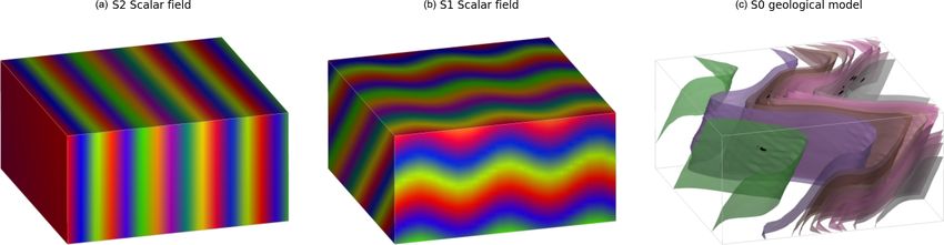
Geosci. Model Dev., 14, 3915–3937, 2021 https://doi.org/10.5194/gmd-14-3915-2021L. Grose et al.: LoopStructural 1.0: time-aware geological modelling 3927 Figure 8. Structural data for refolded fold: (a) observations of S2, (b) observations of S1 showing interpolated scalar field of S2 and (c) observations of S0 showing interpolated scalar field of S1. Figure 9. F2 S plot showing the fold rotation angle between observations of S1 and the fold frame S2. The structural observations were sampled from a synthetic 4.3 Integration with map2loop topographical horizon from three outcrop locations. The ax- ial foliation to F2, S2, is shown in Fig. 9a. The observations In the final examples we use map2loop (Jessell et al., 2021) of S2 are used to interpolate the major structural feature of as a pre-processor to generate an input dataset from regional the F2 fold frame (Fig. 12a). The axial foliation of F1, S1, geological survey maps, the national stratigraphic database is shown in Fig. 9b, and the scalar field value of the interpo- and a global digital elevation model. map2loop creates lated S2 is shown on the map. The fold rotation angle for F2 a set of augmented data files that can be used to build a is calculated by finding the angle between the interpolated geological model in LoopStructural. The class method (Ge- S2 field and the folded S1 field and is shown in the S plot ologicalModel.from_map2loop_directory(m2l_directory, for Fig. 10a. The red curve in Fig. 10a is a Fourier series that **kwargs)) creates an instance of a GeologicalModel from is automatically fitted to the observations. The wavelength of a root map2loop output directory. We will demonstrate the the fold is estimated by finding the first peak of the S vari- interface between map2loop and LoopStructural with two ogram (Fig. 10b). Fold constraints are added into the interpo- case studies (1) from the Flinders Ranges in South Australia lation algorithm using this curve to define the geometry of the and (2) from the Hamersley region in Western Australia. fold along the fold axis, and the average intersection lineation The first case study demonstrates the interface between between the S1 foliation and the interpolated S2 field is a map2loop and LoopStructural for a large regional model. proxy for the fold axis. The interpolated scalar field is shown The second case study shows how the conceptual model in Fig. 12b. The observations of S0 are shown in Fig. 9c, and used to generate the input dataset can be varied. the scalar value of the S1 field is shown on the map. The S The first example uses a small study area from South plot for F1 is shown in Fig. 11a and shows two opposing fold Australia using the Geological Survey of South Australia’s limbs in the data points. The red curve shows the Fourier se- open-access datasets (GSSA, 2020). The model area covers ries that characterises the geometry of the fold along the fold approximately 85 km by 53 km within the Finders Ranges in axis and indicates that there are two unobserved fold hinges South Australia. The stratigraphic units within this area are away from the data points. These constraints are added into shown in Fig. 13a, and the outcropping geology is shown the implicit model, and the scalar field is shown in Fig. 12c. in the geological map (Fig. 13b); the patches of the map https://doi.org/10.5194/gmd-14-3915-2021 Geosci. Model Dev., 14, 3915–3937, 2021
3928                                                        L. Grose et al.: LoopStructural 1.0: time-aware geological modelling

Figure 10. F1 S plot showing the fold rotation angle between observations of S0 and the fold frame S1.

Figure 11. Scalar fields: (a) S2, (b) S1 and (c) bedding.

without any geological units represent shallow Tertiary and            **kwargs)) class method, meaning the geological model can
Quaternary cover. map2loop extracts basal contacts from                be produced without any user input.
the outcropping geological units and estimates the layer                  The resulting geological model surfaces are shown in
thicknesses shown in the stratigraphic column. Within this             Fig. 14 where the surface represents the base of a strati-
map area all of the stratigraphic groups share a similar               graphic group and are coloured using the stratigraphic col-
deformation history and area modelled as a single super-               umn (Fig. 13a). The faults in the model are interpolated us-
group. The cumulative thickness is estimated for all of the            ing a Cartesian grid with 50 000 elements and are interpo-
stratigraphic horizons relative to the Pound Subgroup and is           lated using the finite-difference interpolator, and the interpo-
used to constrain the value of the implicit function. There            lation matrix is solved using the pyamg algorithmic multi-
are 15 faults within the model area with limited geometrical           grid solver (Olson and Schroder, 2018). Stratigraphy is inter-
information constraining only the map trace of the faults. As          polated using a finer mesh with 500 000 elements using the
a result, the faults are assumed to be vertical with a vertical        finite-difference interpolator and also using pyamg. Using a
slip direction, and the displacements are estimated from the           workstation laptop with an i7 processor and 32gb of RAM
geometry on the geological map using map2loop. The geom-               the data processing using map2loop takes approximately
etry of the fault can be changed within LoopStructural and             1 min, building the implicit model takes approximately 8 min
map2loop to explore the uncertainty space. The overprinting            and the rendering of the surfaces on a (200 × 200 × 100)
relationships of the faults are estimated from the geological          Cartesian grid takes 3 min. The intersection of the solid ge-
map using map2loop by analysing the intersection between               ological model and the map surface is shown in Fig. 13c,
faults on the geological map. The estimated overprinting               allowing for a comparison with the input dataset. The geo-
relationships are used to constrain the order of the faults            logical model has interpolated the geological packages un-
in the geological model. The scalar field representing the             derneath the surficial deposits.
supergroup is interpolated after the observations of the strati-          In the second example we use map2loop to process a small
graphic horizon (contacts and orientation measurements)                area of the Turner Syncline in the Hamersley region in West-
are un-faulted using the calculated fault displacements.               ern Australia using data provided by the Geological Sur-
The modelling workflow is all encapsulated in the (Ge-                 vey of Western Australia (GSWA) (2016). The model area
ologicalModel.from_map2loop_directory(m2l_directory,                   is 12 km × 13 km and includes three faults. The default as-
                                                                       sumption by map2loop is that the faults are vertical and are

Geosci. Model Dev., 14, 3915–3937, 2021                                                  https://doi.org/10.5194/gmd-14-3915-2021
You can also read