Joint estimation of atmospheric and instrumental defects using a parsimonious point spread function model - Astronomy & Astrophysics
←
→
Page content transcription
If your browser does not render page correctly, please read the page content below
A&A 643, A58 (2020)
https://doi.org/10.1051/0004-6361/202038679                                                                                                              Astronomy
c O. Beltramo-Martin et al. 2020                                                                                                                          &
                                                                                                                                                         Astrophysics

 Joint estimation of atmospheric and instrumental defects using a
            parsimonious point spread function model
    On-sky validation using state of the art worldwide adaptive-optics assisted
                                   instruments
                     Olivier Beltramo-Martin1,2 , Romain Fétick2,1 , Benoit Neichel1 , and Thierry Fusco2,1

     1
         Aix Marseille Univ, CNRS, CNES, LAM, Marseille, France
         e-mail: olivier.martin@lam.fr
     2
         DOTA, ONERA, Université Paris Saclay, 91123 Palaiseau, France

     Received 17 June 2020 / Accepted 31 July 2020

                                                                                    ABSTRACT

     Context. Modeling the optical point spread function (PSF) is particularly challenging for adaptive optics (AO)-assisted observations
     owing to the its complex shape and spatial variations.
     Aims. We aim to (i) exhaustively demonstrate the accuracy of a recent analytical model from comparison with a large sample of
     imaged PSFs, (ii) assess the conditions for which the model is optimal, and (iii) unleash the strength of this framework to enable the
     joint estimation of atmospheric parameters, AO performance and static aberrations.
     Methods. We gathered 4812 on-sky PSFs obtained from seven AO systems and used the same fitting algorithm to test the model
     on various AO PSFs and diagnose AO performance from the model outputs. Finally, we highlight how this framework enables the
     characterization of the so-called low wind effect on the Spectro-Polarimetic High contrast imager for Exoplanets REsearch (LWE;
     SPHERE) instrument and piston cophasing errors on the Keck II telescope.
     Results. Over 4812 PSFs, the model reaches down to 4% of error on both the Strehl-ratio (SR) and full width at half maximum
     (FWHM). We particularly illustrate that the estimation of the Fried’s parameter, which is one of the model parameters, is consistent
     with known seeing statistics and follows expected trends in wavelength using the Multi Unit Spectroscopic Explorer instrument
     (λ6/5 ) and field (no variations) from Gemini South Adaptive Optics Imager images with a standard deviation of 0.4 cm. Finally, we
     show that we can retrieve a combination of differential piston, tip, and tilt modes introduced by the LWE that compares to ZELDA
     measurements, as well as segment piston errors from the Keck II telescope and particularly the stair mode that has already been
     revealed from previous studies.
     Conclusions. This model matches all types of AO PSFs at the level of 4% error and can be used for AO diagnosis, post-processing,
     and wavefront sensing purposes.
     Key words. instrumentation: adaptive optics – methods: data analysis – techniques: image processing – atmospheric effects –
     methods: analytical

1. Introduction                                                                                 performance. From the PSF, we can identify the major con-
                                                                                                tributors to the AO residual error (Beltramo-Martin et al. 2019;
Adaptive optics (AO, Roddier 1999) is a game changer in                                         Ferreira et al. 2018; Martin et al. 2017). Secondly, the image
the quest for high-angular resolution, especially for ground-                                   delivered by an optical instrument depends on both the sci-
based astronomical observations that face the presence of wave-                                 ence object we want to characterize and the PSF. In order
front aberrations introduced by the atmosphere (Roddier 1981).                                  to estimate the interesting astrophysical quantities, one can
Thanks to AO, the point spread function (PSF) delivered by an                                   either use a deconvolution technique (Fétick et al. 2020, 2019a;
optical instrument is much narrower, by a factor up to 50 on the                                Benfenati et al. 2016; Flicker & Rigaut 2005; Mugnier et al.
full width at half maximum (FWHM), than the seeing-limited                                      2004; Fusco et al. 2003; Drummond 1998) or include the PSF
scenario (Roddier 1981). Still, some correction residuals per-                                  as part of a model, as is performed in PSF-fitting astrom-
sist and render the AO PSF shape complex to model. Conse-                                       etry/photometry retrieval techniques (Beltramo-Martin et al.
quently, standard parametric models that reliably reproduce the                                 2019; Witzel et al. 2016; Schreiber et al. 2012; Diolaiti et al.
seeing-limited PSFs, such as a Moffat function (Trujillo et al.                                 2000; Bertin & Arnouts 1996; Stetson 1987) and galaxy
2001; Moffat 1969), become inefficient at describing the AO                                     kinematics estimation (Puech et al. 2018; Bouché et al. 2015;
PSF. Moreover, contrary to seeing-limited observations, AO-                                     Epinat et al. 2010) for instance.
corrected images suffer from the anisoplanatism effect (Fried                                       Nevertheless, the PSF is not systematically straightfor-
1982) that strengthens the spatial variations of the PSF on                                     ward to determine from the focal-plane image, particularly for
top of instrument defects. Determining the AO PSF is neces-                                     observations made with a small field of view (FOV), or of
sary for two major reasons. Firstly, understanding and accu-                                    extended objects, crowded populations or with a low signal-
rately modeling the PSF morphology is key to diagnosing AO                                      to-noise ratio (S/N). Alternative methods exist, such as PSF
                                                                                                                                                                            A58, page 1 of 15

               Open Access article, published by EDP Sciences, under the terms of the Creative Commons Attribution License (https://creativecommons.org/licenses/by/4.0),
                                which permits unrestricted use, distribution, and reproduction in any medium, provided the original work is properly cited.
A&A 643, A58 (2020)

reconstruction (Beltramo-Martin et al. 2019, 2020; Wagner et al.       where ρ is the separation vector within the pupil, λ is the imaging
2018; Gilles et al. 2018; Ragland et al. 2018; Martin et al.           wavelength, and ρ/λ is the angular frequencies vector.
2016a; Ragland et al. 2016; Jolissaint et al. 2015; Exposito                The static OTF derives from the instrument pupil mask P(r)
2014; Clénet et al. 2008; Gendron et al. 2006; Veran et al. 1997),     and the optical path difference (OPD) map ∆Static in the pupil
which is potentially very accurate (1% error level). However,          plane, which gives for a monochromatic beam at wavelength λ
this process lacks science verification and requires years to be                        "
fully implemented and operational as a stand-alone pipeline.           h̃Static (ρ/λ) =     P(r)P∗ (r + ρ) exp (2iπ/λ(∆Static (r)
The inherent complexity has inspired several efforts to produce                           P                                            (2)
simpler but still efficient reconstruction techniques (Fusco et al.                     −∆Static (r + ρ))) dr.
2020; Fétick et al. 2019b) that have been fully validated and
are now in operation for Multi Unit Spectroscopic Explorer             The SPHERE/IRDIS data we have treated (see Sect. 3.1 for a
(MUSE) (Bacon et al. 2010) at the Very Large Telescope (VLT).          more complete description) were obtained during PSF calibra-
The analytic AO PSF model described by Fétick et al. (2019b)           tion procedure using an off-axis stars. Therefore, the incom-
has shown spectacular accuracy in reproducing the MUSE Nar-            ing beam was not getting through the focal-plane mask and the
row Field Mode (NFM) PSF as well as the PSF of the Zurich              pupil mask model results from the multiplication of the apodizer
Imaging Polarimeter (ZIMPOL) (Schmid et al. 2018) that equips          (amplitude) function A and the Lyot stop L (Soummer 2005) as
the Spectro-Polarimetic High contrast imager for Exoplanets            follows
REsearch (SPHERE) instrument (Beuzit et al. 2019) PSF and is
an excellent candidate to rethink the way we perform PSF recon-        P(r) = A(r).L(r).                                                 (3)
struction, with a single flexible algorithm that complies with all
kinds of AO correction. However, several questions arise as to         The 2D functions A(r) and L(r) are illustrated in Fig. 1.
its capabilities. Does this model really match any type of AO               In this paper, we split the static aberration contribution in two
PSF, regardless of the observing conditions and even at very           terms: the Non Common Path Aberrations (NCPA) calibration
high Strehl-ratio (SR)? How much accuracy can we expect in             (non-coronagraphic) noted ∆NCPA (Jia et al. 2020; Vigan et al.
a statistical sense and what are the fundamental limits? Can we        2019; Lamb et al. 2018; Vassallo et al. 2018; N’Diaye et al.
improve the description of the PSF in the presence of static aber-     2016; Sitarski et al. 2014; Jolissaint et al. 2012; Sauvage et al.
rations? The goal of this paper is to address these questions by (i)   2011; Robert et al. 2008; Mugnier et al. 2008; Blanc et al. 2003;
providing an exhaustive demonstration that this model complies         Fusco et al. 2003), to which is added another contribution
with any type of AO system, telescope, and in optical and near         decomposed over a modal basis M to be specified. This latter
infrared (NIR) wavelengths, (ii) assessing conditions for which        could be simply Zernike modes over the whole pupil or per pupil
the model is optimal for representing an AO PSF, and (iii) show-       area delimited by the spiders, so as to include potential LWE that
ing that this framework is robust enough to enable the joint esti-     may introduce severe asymmetries in the PSF structure. Analy-
mation of AO residual and instrumental aberrations. In Sect. 2,        ses of SPHERE images (Milli et al. 2018; Sauvage et al. 2016,
we present the theoretical background and the model description        2015) showed that the LWE mainly introduces piston, tip, and
as well as some upgrades we have implemented so as to treat            tilt differential aberrations between pupil areas separated by the
new types of data and include static-aberration fitting. In Sect. 3,   spiders, which represents 12 parameters to be adjusted. Also, for
we present a statistical analysis of the model accuracy over 4812      segmented pupil telescopes like Keck telescopes, this basis can
PSFs with a discussion on the parameter estimates. Finally, in         be segment piston or petal modes (Ragland 2018). We analyze
Sect. 4, we illustrate how the present model allows joint esti-        the capacity of this model to identify such aberrations in Sect. 4.
mation of atmospheric conditions, AO performance and static            The static OPD is calculated following
aberrations, caused by the low wind effect (LWE) on SPHERE                                         nm
or segment cophasing error at Keck.
                                                                                                   X
                                                                       ∆Static (r) = ∆NCPA (r) +         µStat (k)Mk (r),                (4)
                                                                                                   k=1

2. PSF model                                                           where µStat (k) and Mk are respectively the coefficient and 2D
This model was originally introduced by Fétick et al. (2019b)          shape of the kth mode over nm modes. To include segment piston
and validated on SPHERE/ZIMPOL and MUSE NFM data. In                   errors, Mk must be defined as the pattern formed by the kth seg-
order to increase the range of applicability of such a model, we       ment (36 in total for the Keck pupil) and ak is the piston value
upgraded it by including (i) the model of the Apodized Lyot            in meters. Eventually, one may estimate both the atmospheric
Coronagraph (APLC, Soummer 2005) used on SPHERE (focal-                parameters and static coefficients and we illustrate such a joint
plane mask not considered) (ii) additional degrees of freedom          estimation on Keck data in Sect. 4.1.
to adjust static aberrations over a specific modal basis, which            Finally, the description of the AO residual spatial filter k̃AO in
can be Zernike modes described on the pupil, tip-tilt and pis-         Eq. (1) relies on two assumptions, which are, (i) the exposure is
ton modes for each pupil area delimited by the spiders so as           infinitely long, and (ii) the residual phase is a Gaussian statistical
to describe the so-called LWE or piston modes for each pupil           process. Thus, k̃AO is fully described by the residual phase power
segment (Laginja et al. 2019; Leboulleux et al. 2018; Ragland          spectrum density (PSD) as follows (Roddier 1981):
2018).                                                                 k̃AO (ρ/λ) = exp (−0.5 × DAO (ρ, λ)) ,
    First of all, the model assumes the stationarity of the phase of
the electric field in the pupil plane (Roddier 1981), which allows     DAO (ρ, λ) = 2 × (BAO (0, λ) − BAO (ρ, λ)) ,                      (5)
the system optical transfer function (OTF) to be split into a static   BAO (ρ, λ) = F [WAO (k)] ,
part h̃Static (telescope + internal aberrations) and an AO residual
spatial filter k̃AO as follows,                                        where DAO , BAO , and WAO are the residual phase structure
                                                                       function, autocovariance function, and PSD respectively, k is the
h̃(ρ/λ) = h̃Static (ρ/λ)k̃AO (ρ/λ),                             (1)    spatial frequencies vector and F [x] is the 2D Fourier transform
A58, page 2 of 15
O. Beltramo-Martin et al.: Joint estimation of atmospheric and instrumental defects
contaminates wavefront measurements due to the WFS discrete
sampling (Bond et al. 2018a; Correia & Teixeira 2014; Jolissaint
2010; Rigaut et al. 1998).
– A is the total energy in nm2 contained in the Moffat PSD
model (constant C not included) and thus characterizes the AO
residual wavefront error that connects to the PSF SR, that is,
the intensity of the PSF peak compared to the diffraction-limit
scenario.
– α x , αy , and θ govern the elongation and skewness of the
PSD as well as the direction of the elongation thanks to the angle
θ. The PSD FWHM is proportional to α x , αy parameters; for the
Fig. 1. From left to right: pupil plane apodizer and Lyot stop used same amount of energy, a PSD with a larger FWHM indicates
during SPHERE/IRDIS observations with the N_ALC_YJH_S APLC that the PSD flattens and the correction homogenizes across spa-
(Vigan et al. 2010). tial frequencies.
– β represents the asymptotic slopes of the PSD at
large spatial frequencies within the AO correction radius.
of x. In Fétick et al. (2019b), the PSD is described as a split From Fourier analysis of AO performance (Bond et al. 2018a;
function to separate the AO-corrected spatial frequencies from Correia & Teixeira 2014; Jolissaint 2010; Rigaut et al. 1998), we
the uncorrected frequencies that follow a Kolmogorov’s −11/3 know that the PSD pattern introduced by the wavefront mea-
power law (Kolmogorov 1941) surement noise follows a k−2 power law for WFSs sensitive to
the first order derivative of the wavefront such as the Shack-
M(k, A, α x , αy , θ, β) + C for k ≤ kAO
Hartmann. Asymptotically, we would have β = 1 for a Shack-
WAO (k) = , (6)
0.023r−5/3 k−11/3 for k > kAO
0
Hartmann based AO system if the measurement noise is the
only error in the wavefront reconstruction process. Moreover, in
where k = |k|, r0 is the Fried parameter (Fried 1966), kAO the the situation of an AO system correcting all atmospheric aber-
equivalent AO cut-off frequency beyond which the AO correc- rations with the same relative level (which does not occur as
tion no longer occurd, C a constant value and M an asymmet- the sensitivity of the wavefront sensor is aberration-dependent
ric Moffat function (Moffat 1969) that depends on five shape Fauvarque et al. 2016), we would obtain β = 11/6 ' 1.83
parameters A, α x , αy , θ, and β and on the spatial frequency vector according to the von Kármánn expression of the atmospheric
k = (k x , ky ) as follows, PSD (von Karman 1948). Nevertheless, larger values of β can
be observed. Indeed, for very large values of β, the Moffat distri-
M(k, A, α x , αy , θ, β) = bution converges towards a Gaussian shape (Trujillo et al. 2001),
ψ×A as does the PSF consequently. We expect this behavior with poor
, tip-tilt correction for instance or in the presence of strong tele-
(1 + (k x cos(θ) + + (ky cos(θ) − k x sin(θ))2 /α2y )β
ky sin(θ))2 /α2x
scope wind-shake or telescope/dome vibrations. As a summary,
(7) β should usually range between 1 and 1.83 for nominal AO
correction but can reach higher values in the presence of non-
where ψ is a normalization factor that ensures that the integral
atmospheric aberrations.
of the Moffat function over the AO-corrected area is given by A:
We illustrate in Fig. 2 azimuthal profiles of PSDs and corre-
(Fétick et al. 2019b)
sponding PSFs for various sets of model parameters. This figure
β−1 1 shows clearly how r0 drives the PSF halo and how the param-
ψ= . (8) eter A increases the area underneath the PSD curve, which cor-
πα x αy (1 − (1 + kAO
2
/(α x αy ))1−β
responds to the residual wavefront error. We also observe that
Contrary to the classical use of a Moffat function in astron- a larger value of β sharpens the PSD. Knowing that the total
omy (Trujillo et al. 2001; Moffat 1969), we stress that the Mof- energy remains constant, this situation corresponds to less effi-
fat function used in the present model serves in the description cient low-order modes compensation. Finally, a larger value of
of the PSD and not the focal-plane PSF. This latter is deduced α increases the PSD FWHM and distributes more energy over
by the inverse Fourier transform of the OTF given in Eq. (1). the highest AO-correct modes. The shape of the PSF is mainly
Consequently, the PSF FWHM is actually driven by parameters conditioned by parameters A and r0 , which are the two most sig-
A and r0 rather than α x , αy , and β. In order to really capture the nificant parameters of this model. Parameters C, α, θ, and β are
physical meaning of this model, below we present a description secondary parameters that shape the PSD in order to more accu-
of each of the seven parameters that the model relies on and their rately reproduce the PSF structure in various observing condi-
impact on the PSF: tions and especially in the presence of sub-optimal AO control or
– r0 constrains the uncorrected PSD that corresponds to the non-atmospheric aberrations. Henceforth, this model is a combi-
PSF wings, that is, the part of the PSF that remains untouched nation of a PSF determination tool and an AO diagnosis facility
by any AO correction. For a system with nact × nact actuators to gathered up together into a single and parsimonious analytical
compensate for the incoming wavefront, this breaking occurs in framework.
the focal plane at approximately nact × λ/(2D), with D the pri-
mary mirror diameter and for a Nyquist-sampled PSF (Roddier
1999). 3. Model versus reality: statistical validation
– C is a constant value that changes the gap between the 3.1. Overview of data
AO-corrected part and the uncorrected high-spatial frequencies.
This parameter plays a major role near the AO cutoff in both We aim to provide the most exhaustive on-sky validation
the PSD and PSF planes, and compares to the aliasing error that of the PSF analytical and parsimonious model proposed by
A58, page 3 of 15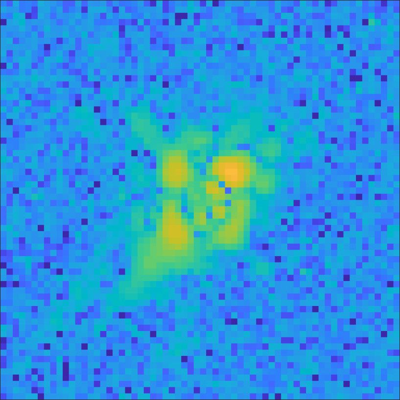
A&A 643, A58 (2020)

Fig. 2. Azimuthal average in log-log scale of the PSD (left) and the PSF (right) obtained with four different settings for the model parameters,
assuming that the PSD is symmetric, i.e. α x = αy = α and θ = 0. No static aberrations were added here and the parameter C was set to
C = 10−4 rad2 m2 . The PSF maximum is normalized to the SR value.

Fétick et al. (2019b). To achieve this goal, we collected 4812           frame, and correct for the flat-field. These data are particularly
PSFs obtained from different observatories, AO systems, AO               useful for testing the model in optical wavelengths and under
modes and spectral bands covering optical and NIR wavelengths.           strong atmospheric residual regime.
The GALACSI/MUSE and GeMS/GSAOI instruments deliver
simultaneous PSFs at different wavelengths and field positions               SPHERE/IRDIS@VLT.            A     total  of   237      PSFs
respectively. If we consider a single PSF for each observation           were obtained from the SPHERE Data Centre client
they produce, we obtain a total of 1880 PSFs. However, although          (Delorme et al. 2017) using the Keyword Frame type set
the realizations of atmospheric residual wavefront are not inde-         to IRD_SCIENCE_PSF_MASTER_CUBE. These PSFs were
pendent from a PSF to another within the same observation,               acquired over the last five years with the N_ALC_YJH_S APLC
these data allow to test the model in the presence of chro-              (Vigan et al. 2010) during PSF calibration and with a pixel scale
matic and field-dependent instrumental aberrations. In order to          of 12.5 mas pixel−1 . These data were collected using the dual
conserve the same fitting process for all data, we have fitted           band filters DB_H23, and DB_K12, and they are useful for
each PSF with the same starting point and regardless the results         testing the model under very high SR regime and for validating
obtained on another PSF acquired during the same observation.            the LWE retrieval presented in Sect. 4.2.
A description of each data set is given below
                                                                             Keck AO/NIRC2@Keck II. We obtained 355 PSFs using
    SPHERE/ZIMPOL@VLT. SPHERE is a facility at the VLT                   the narrow field mode of NIRC2 with a pixel scale of
that was installed in 2015 and relies on an extreme AO (EXAO)            9.94 mas pixel−1 and using the Fe II and K cont filters. The Keck
system (Sphere Ao for eXoplanets Observations; Fusco et al.              AO system on the Keck II telescope was operated in single con-
2016; Sauvage et al. 2015) to deliver a very efficient atmo-             jugated AO (SCAO) mode using a natural (Wizinowich et al.
spheric correction level to three science instruments, which             2000) or an on-axis laser (Wizinowich et al. 2006) guide star.
are ZIMPOL (Schmid et al. 2018), IRDIS (Dohlen et al. 2008),             These PSFs were obtained during PSF reconstruction engineer-
and IFS (Claudi et al. 2014). This set of data is composed of            ing nights in 2013 and 2017 (Ragland et al. 2018, 2016) and
two subsets of PSFs from SPHERE/ZIMPOL. The first (26                    such data are especially useful to validate the model under the
PSFs) was obtained from observations of NGC 6121 in 2019                 influence of remaining piston cophasing errors, as we discuss in
(Massari et al. 2020; Beltramo-Martin et al. 2020) with the ZIM-         Sect. 4.1.
POL V-filter (central wavelength 554 nm, width 80.6 nm) and
a pixel scale of 7.2 mas pixel−1 in the context of technical cal-            SOUL/LUCI@LBT. These data were delivered in 2020 from
ibrations1 granted after the 2017 ESO calibration workshop2 .            the to two LUCI NIR spectro-imagers assisted with the pyramid
The second set of 18 PSFs was acquired in 2018 with the N_R-             SCAO (PSCAO) SOUL AO system (Pinna et al. 2016) driven
filter (central wavelength 645.9 nm, width 56.7 nm) and a pixel          by a pyramid WFS (Ragazzoni & Farinato 1999). These PSFs
scale of 3.6 mas pixel−1 during the ESO Large Program (ID                were acquired using the H filter (1.653 µm) and with a sam-
199.C-0074, PI P. Vernazza) (Vernazza et al. 2018). The data             pling of 15 mas pixel−1 . Although few (11 for our purpose) data
were reduced using the SPHERE Data and Reduction Handling                sets have been obtained so far in comparison to others systems,
pipeline (DRH) to extract the intensity image, subtract a bias           these PSFs pave the way to a demonstration of PSF determina-
                                                                         tion strategies in the presence of a pyramid WFS, which will be
1
  ESO program ID of observations: 60.A-9801(S).                          the baseline for the SCAO mode of HARMONI (Thatte 2017),
2
  See              http://www.eso.org/sci/meetings/2017/                 MICADO (Davies et al. 2016) and METIS (Hippler et al. 2019)
calibration2017                                                          on the future 39 m Extremely Large Telescope (ELT).
A58, page 4 of 15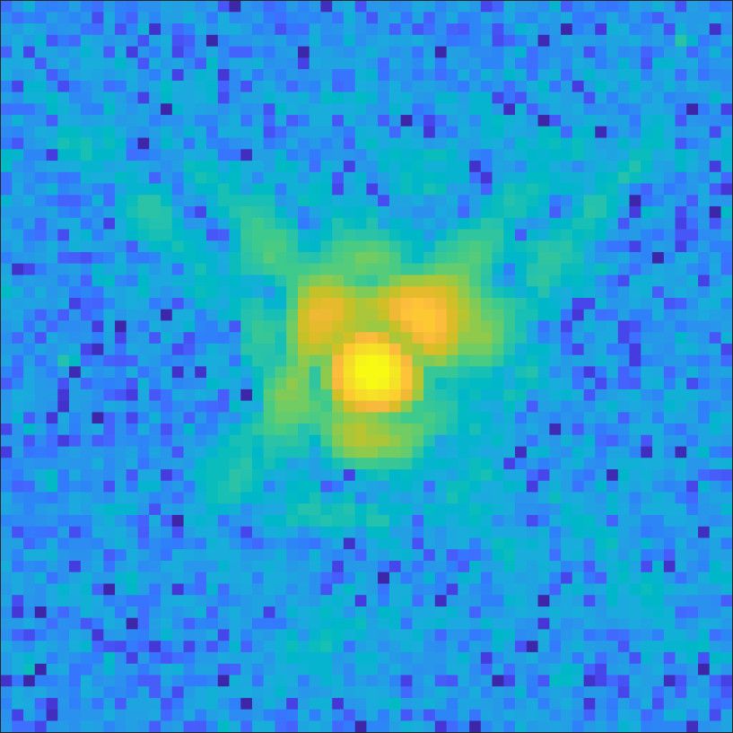
O. Beltramo-Martin et al.: Joint estimation of atmospheric and instrumental defects

    CANARY/CAMICAZ@WHT. CANARY (Gendron et al.                              – Define a model of the image including the PSD degrees
2010; Myers et al. 2008) was designed as a pathfinder for              of freedom (no static aberrations retrieval) µAO as well as four
demonstrating the reliability and robustness of the multi-object       additional scalar factors δ x , δy , γ, and ν in order to finely adjust
AO (MOAO) concept proposed for assisting very large field              the PSF position, flux, and constant background level,
(>10 ) multi-object spectrographs, such as MOSAIC for the ELT                                           h
(Hammer et al. 2016). Thanks to 26 nights of commissioning,             d̂(µAO , γ, δ x , δy , ν) = γ.F h̃Static .k̃AO (µAO )
tests, and validation, we collected 1268 PSFs in H-band and                                                                           i    (9)
with a sampling of 30 mas pixel−1 using the NIR detector                                            × exp 2iπ × (ρ x δ x /λ + ρy δy /λ) + ν.
CAMICAZ (Gratadour et al. 2014). These data were obtained
                                                                       The image model is calculated over a given number of pixels that
during phase B (Martin et al. 2017; Morris et al. 2014, 2013;
                                                                       is 10% larger than the on-sky images so as to mitigate aliasing
Martin et al. 2013), which was dedicated to the demonstration
                                                                       effects due to the Fast Fourier Transform algorithm. The size of
of MOAO relying jointly on four (Rayleigh) laser guide star
                                                                       the on-sky image support is instrument-dependent and truncated
(LGS) and up to three natural guide star (NGS) in a 1’ FOV to
                                                                       in order to mitigate the noise contamination. When possible, we
perform the tomography using the Learn & Apply technique
                                                                       crop the on-sky image to conserve a FOV up to twice the AO
(Laidlaw et al. 2019; Martin et al. 2016b; Vidal et al. 2010).
                                                                       cutoff.
Among this quite large set of data, we have 522 PSFs in SCAO
                                                                           – Define a criterion to minimize
mode, 128 PSFs in ground layer AO (GLAO) mode and 618
MOAO PSFs. Such an archive is useful for testing the model on
                                                                                                   X     h                                    i2
                                                                        ε(µAO , γ, δ x , δy , ν) =   Wi j d̂i j (µAO , γ, δ x , δy , ν) − di j , (10)
a 4.2 m class telescope and on tomographic and laser-assisted                                    i, j
AO-corrected-PSFs.
   GALACSI/MUSE NFM@VLT. MUSE is the ESO VLT
                                                                       where di j is the (i, j) pixel of the 2D image and Wi j the weight
second-generation wide-field integral field spectrograph operat-       matrix defined by
ing in the visible (Bacon et al. 2010), covering a simultaneous                          1
spectral range of 465–930 nm and assisted by the ESO Adap-             Wi j =                        .                                         (11)
                                                                                max di j , 0 + σ2ron
                                                                                   n        o
tive Optics Facility (AOF, Oberti et al. 2018; Arsenault et al.
2008) including the GALACSI module (Ströbele et al. 2012).
                                                                       The weight matrix accounts for the noise variance, that is, both
We focused our analysis on the narrow field mode (NFM)
                                                                       photon noise and read-out noise, and allows us to maximize the
of MUSE, which delivers a laser tomography AO (LTAO)-
                                                                       robustness of the fitting process (Mugnier et al. 2004).
corrected field covering a 7.500 × 7.500 FOV, providing near-
                                                                           – Perform the minimization using a nonlinear and iterative
diffraction-limited images with a sampling of 25 mas pixel−1 .
                                                                       recipe based on the trust-reflective-region algorithm (Conn et al.
These PSFs were obtained during the commissioning phase in
                                                                       2000). We did not use specific regularization techniques on top
2018 and are particularly useful for analyzing the model outputs
                                                                       of the weighting matrix as we have taken care of selecting good
with respect to the wavelength and demonstrating that the model
                                                                       S/N images.
also complies with under-sampled PSFs. Also, we performed a
spectral binning to reach a spectral width of 5 nm (91 PSFs per
cube if we remove the notch filter wavelengths), resulting in a        3.3. PSF model accuracy
total of 1986 PSFs.
                                                                       In Fig. 3, we present a visual comparison of on-sky PSFs, best-
   GEMS/GSAOI@GEMINI. The Gemini South Adaptive                        match model and residual map for the seven instruments con-
Optics Imager (GSAOI) is a NIRd camera that benefits the cor-          sidered in this analysis. The model adapts to any kind of AO
rection provided by the Gemini Multi-conjugate Adaptive Optics         correction; the maps of residuals are visually similar to first
(MCAO) System (GeMS, Neichel et al. 2014; Rigaut et al.                order among all systems. On the Keck AO/NIRC2 image, we
2014) on Gemini South. It delivers near-diffraction-limited            see some structures that are static speckles, probably introduced
images in the 0.9 – 2.4 µm wavelength range in a large FOV of          by a remaining cophasing error, and residual NCPA as illus-
8500 × 8500 . From the Gemini archive (Hirst & Cardenes 2017),         trated in Sect. 4.1. On SOUL/LUCI and CANARY/CAMICAZ
we assembled a catalog of 911 isolated and nonsaturated PSFs           images, we also see a persistent pattern that can be explained
extracted from 60 images of Trumpler 14 acquired in 2019               by the presence of static aberrations not included in the
and using the J, H, K, and Brγ filters with a pixel scale of           model and the exposure time that was not sufficiently long
20 mas pixel−1 (P.I. M. Andersen, observation program: GS-             (a few seconds of exposure) to average the atmospheric
2019A-DD107). These data are particularly useful for investi-          speckles.
gating model parameters variations across a MCAO-corrected                  In Fig. 4, we illustrate the SR and FWHM obtained from the
FOV.                                                                   fitted model versus sky image-based estimates. The same algo-
    In total, we created a dictionary of 4812 PSFs covering sev-       rithms (OTF integral for the SR, interpolation+contour for the
eral observatories, AO correction types, optical and NIR wave-         FWHM) were used to calculate these metrics regardless of the
lengths, as summarized in Table 1. Having this diversity of data       nature of the data, either sky image or model. For all systems,
is important for spanning the full range of possible AO cor-           we observe a remarkable correlation and a similar dispersion on
rection levels and assessing which conditions must be met to           both SR and FWHM and for all observing conditions, AO modes
achieve an accurate PSF representation.                                and AO correction levels. For very high SR values obtained with
                                                                       SPHERE/IRDIS, we start observing an overestimation of the SR
3.2. PSF fitting                                                       suggesting that the model cannot fully retrieve some patterns in
                                                                       the image. At this level of correction, the instrumental contribu-
In order to fit the model over the image and retrieve the associ-      tion (residual NCPA, LWE for instance) of the PSF may dom-
ated parameters, we followed the same strict process for each of       inate the PSF morphology while they are not included in the
the 4812 PSFs in our dictionary, which is described as follows         model, as for all 4812 handled data sets. Consequently, in order
                                                                                                                                 A58, page 5 of 15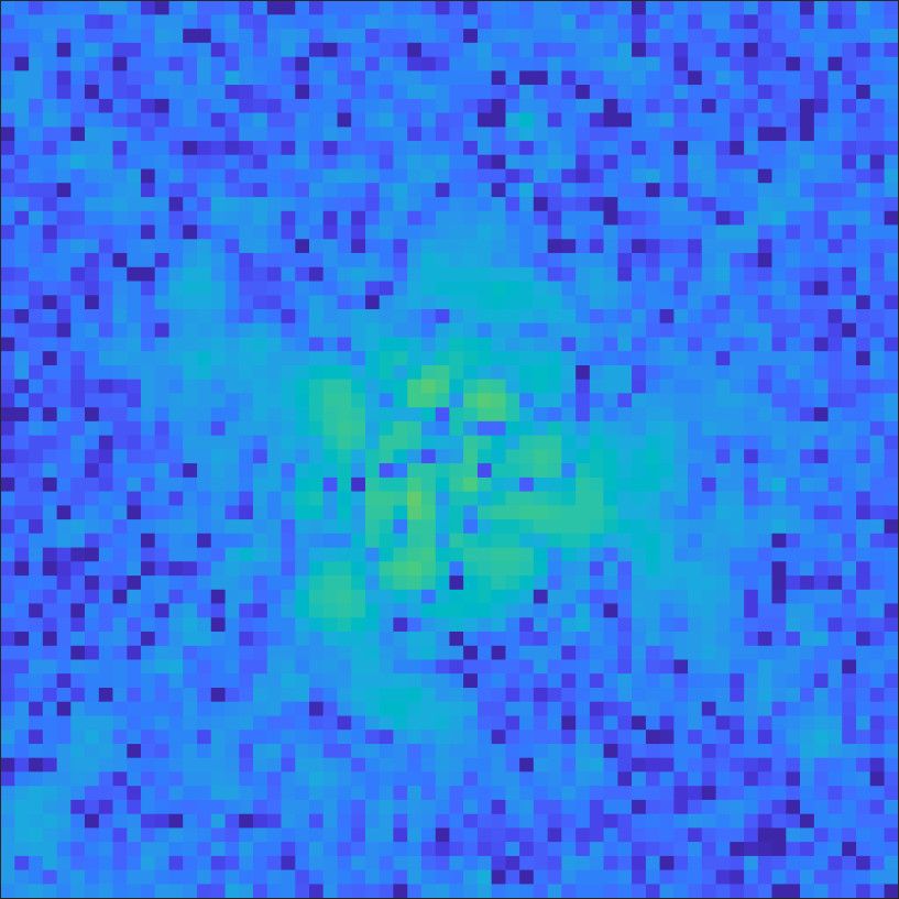
A&A 643, A58 (2020)

Table 1. Summary of PSFs obtained and processed for the analysis presented in this paper.

                    System              AO Mode       λ range (µm)     # PSFs                      Specificity
            SPHERE/ZIMPOL                EXAO          0.55 to 0.65      44              NGS, High Order AO system
             SPHERE/IRDIS                EXAO          1.65 to 2.2      237             NGS-AO residual NCPA/LWE
            KECK AO/NIRC2                 SCAO          1.65 to 2.2     355       Natural and Laser assisted AO/Segmentation
               SOUL/LUCI                 PSCAO             1.65          11                High Order Pyramid WFS
           CANARY/CAMICAZ                MOAO              1.65         1268                      4.2 m pupil
            GALACSI/MUSE                  LTAO         0.46 to 0.93     1986       Spectro-imager and undersampled image
              GEMS/GSAOI                 MCAO          1.12 to 2.2      911                        Large fov
Notes. In total, the model has been tested over 4812 PSFs.

Fig. 3. Two dimensional comparison in log scale and over 64 × 64 pixels of (top) observed PSFs, (middle) fitted model, and (bottom) residual
map for multiple types of AO systems and instruments working in either visible or NIR wavelengths. From left to right: SPHERE/ZIMPOL,
SPHERE/IRDIS with the apodizer and the Lyot stop (no focal plane mask), Keck AO/NIRC2, SOUL/LUCI, CANARY/CAMICAZ in MOAO
mode, GALACSI/MUSE NFM, and GEMS/GSAOI. All PSFs have been normalized to the sum of pixels.

to guarantee an SR and FWHM accuracy at a few percent, it is            3.4. Exploitation of the model outcomes for diagnosing
not necessary to include a precise model of these instrumental               observing conditions and AO performance
defects for AO systems delivering SR up to ∼80%. We confirm
this assumption in Sect. 4. By calculating the relative difference      As discussed above, fitting the shape of the residual phase PSD
((xmodel − xsky )/xsky ) on SR and FWHM values over all the 4812        allows to retrieve atmospheric parameters and AO performance.
data sets, we measure a bias and a standard deviation (std) value       Therefore, the goals in this section are to (i) confirm that the
of 0.7% and 4.0% on the SR estimation and −0.8% and 4.6%                output parameters r0 and A follow expected trends and give con-
on the FWHM estimation. These numbers indicate that there is            fidence in the retrieval process, and (ii) provide statistics on α, β
a marginal performance overestimation of 1% from the model              parameters to asses which values they should reach for a nominal
(larger SR, lower FWHM), which fits the measurements uncer-             AO correction and thus discriminate situations of sub-optimal
tainty envelopes. As a result, this model achieve a PSF recovery        AO correction. We have excluded the parameter θ from this anal-
at a 4% level.                                                          ysis as it corresponds to a PSF orientation only.
     Table 2 provides statistical results of the estimated SR and
FWHM PSFs for all instruments, including the median values for          3.4.1. Primary parameters estimates
all observations and the Pearson correlation factor. As suggested
by Fig. 4, there is no specific bias, except for SPHERE/IRDIS           The seeing is estimated from the PSF wings fitting relying on
for reasons mentioned above, as well as for SOUL/LUCI owing             a Kolmogorov expression of the PSD. This measurement tech-
to the small amount of data we have access to so far. Over-             nique has proven to be robust (Fétick et al. 2019b) as it consists
all, we conclude that (i) the model becomes biased for very             in determining a single parameter from a significant number of
high SR observations (SR > 80%), calling for the introduction           pixels. Thanks to the large redundancy across the pixels of the
of instrumental defects to improve the model accuracy, (ii) the         spatial signature that the algorithms is seeking out, this approach
SR is estimated with a 1-σ precision of 1%, and (iii) the FWHM          still gives meaningful results with moderate S/N in comparison
is estimated with a 1-σ precision of 3 mas, which correspond            to external profilers (Fétick et al. 2019b). However, contrary to
to approximately to one-fifth down to one-tenth the pixel scale         these latter, this focal-plane-based seeing determination includes
depending on the instrument.                                            all turbulence effects that contribute to impact the PSF wings,

A58, page 6 of 15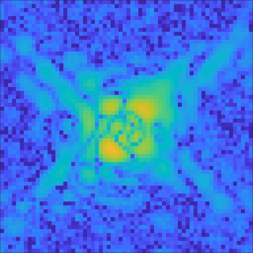
O. Beltramo-Martin et al.: Joint estimation of atmospheric and instrumental defects

Fig. 4. Image SR/FWHM versus the same metrics retrieved on the fitted image using the same estimation process and for the 4812 PSFs treated
for this analysis. Error bars on the SR are obtained from calculations presented in Martin et al. (2016a). Error bars on the FWHM are given from
the contour estimation on interpolated images that are oversampled by up to a factor four to quantify the FWHM more accurately.

Table 2. Individual statistics per system and imaging wavelength on SR and FWHM estimates.

        System                   λ (µm)                            SR (%)                                           FWHM (mas)
                                                 Median         Bias        Std       Pearson       Median          Bias     Std       Pearson
 SPHERE/ZIMPOL                    0.55             6.2          0.5         0.3        0.998           32           −4.2     0.9        0.995
                                  0.64            12.4           0         0.38        0.999           26             1      2.9         0.96
   SPHERE/IRDIS                   1.67             61          −0.2         2.0         0.98           52            0.2     1.4         0.90
                                  2.25            80.0          0.7         3.2         0.98           66            0.8     1.5         0.88
  GALACSI/MUSE                     0.5             2.4         −0.02        0.2        0.993           80           −1.4     2.9        0.997
                                   0.7            10.3          0.1         0.3        0.998           69           −1.7     3.2        0.980
                                   0.9            25.0          0.2         0.7        0.998           58           0.08     5.4         0.90
  KECK AO/NIRC2               1.65 (NGS)          39.4          1.1         0.9        0.998           37           −0.9     0.8        0.994
                               2.2 (LGS)           22           0.7         0.6        0.999           70           −1.9     1.3        0.995
   SOUL/LUCI                      1.65            36.0          1.2         0.5        0.990           55           −2.5     3.3        0.980
CANARY/CAMICAZ                    1.65            23.0          0.1         0.4        0.999          115           −0.1     3.7        0.993
  GEMS/GSAOI                      1.25            13.3           0          0.5        0.994          109           2.0      5.4        0.976
                                  1.64             7.6          0.4         0.5        0.990           98           −4.0     3.2         0.98
                                   2.2            15.6          0.4         0.7        0.994           94           −0.8     4.5        0.970
Notes. The columns “Median” give median values estimated on images, while columns “bias”, “std” and “Pearson” give the median of SR/FWHM
error (in percent) and the Pearson correlation coefficient respectively.

such as the dome seeing (Lai et al. 2019; Conan et al. 2019),            IMM (O’Mahony 2003). We also find consistency with anal-
which the external profilers are not sensitive to as they are apart      ysis by Masciadri et al. (2014) for the Paranal site and by
from the dome. Consequently, estimating the r0 from the focal-           Tokovinin & Travouillon (2006) for Cerro Pachón.
plane image allows to diagnose more accurately the AO perfor-                 In addition, we highlight in Fig. 5 the r0 estimates at zenith
mance in comparison to an external profiler.                             and 500 nm obtained on a single image of GeMS/GSAOI and
     The target here is to verify that the retrieved seeing val-         a single cube of GALACSI/MUSE. For the GEMS/GSAOI case,
ues are consistent with what we know about the observing                 we have r0 measurements obtained from several PSFs distributed
sites. The first verification we made is to analyze statistics on        over the field. Given that r0 is assessed from the PSF wings that
the seeing estimates presented in Table 3. Given that the Keck           contain the non-AO-corrected spatial frequencies, we expect r0
data were acquired in February, August, and September sea-               estimates to be independent of the PSF position in the FOV. Sim-
sons, the median seeing at Mauna Kea is consistent with the              ilarly, we multiplied r0 estimates obtained on GALACSI/MUSE
literature (Ono et al. 2016; Miyashita et al. 2004). Similar obser-      images by a factor (500/λc )6/5 , where λc is the central wave-
vations can be drawn for La Palma by comparing to either                 length of the considered image in the data cube, in order to dis-
CANARY telemetry data (Martin et al. 2016b) or the RoboD-                able the theoretical dependency of r0 with respect to λ.

                                                                                                                              A58, page 7 of 15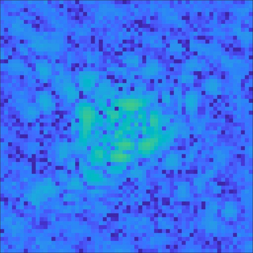
A&A 643, A58 (2020)

Table 3. Median and 1-σ standard-deviation of seeing values retrieved        Figure 7 presents histograms for each system; the β param-
from the PSF-fitting process.                                           eter has a relatively narrow histogram with a peak located at
                                                                        β = 1.82 and a 1-σ standard deviation of 0.6, while the α
                                                                        histograms seem particularly instrument-dependent with val-
           Observing site     Median seeing       1-σ std
                                                                        ues from 0.001 rad.m for efficient AO correction to 1 rad.m for
             Mauna Kea             0.60 00
                                                   0.1300               marginal AO correction (e.g., in the bluest visible wavelengths
            Cerro Pachón           0.6700          0.0900               of MUSE). Our first conclusion here is that an optimized AO
              Paranal              0.8500          0.1500               system should provide a PSD with a β parameter comprised
             La Palma              0.9000          0.2200               between 1 and 1.9, as discussed in Sect. 2. For larger values
                                                                        of β, there is an excess of residual error into low-order spa-
Notes. Seeing values are given at zenith and 500 nm.                    tial frequencies. For instance, we see that on Keck AO/NIRC2
                                                                        images the median β increases from 1.7 up to 2.1 in NGS and
                                                                        LGS modes, respectively, indicating the presence of additional
     Using our model, we retrieve r0 as 14.2 cm ± 0.4 and               low-order modes introduced here mainly from the focal aniso-
10.4 cm ± 0.2 cm for GEMS/GSAOI and GALACI/MUSE,                        planatism (Wizinowich 2012; van Dam et al. 2006). In addition,
respectively. The achieved 3% 1-σ error of our estimates                we have observed cases with β > 2.5 on Keck data due to a
shows that this method is robust and precise compared to                strong wind-shake effect that was enlarging the PSF FWHM by
telemetry-based techniques that typically reach 10% precision           a factor three compared to nominal performance. Both α and β
(Jolissaint et al. 2018).                                               parameters grow up in the presence of strong wind shake and
     For completeness, Fig. 6 shows histograms for the A param-         are wavelength dependent as we see on GALACSI/MUSE his-
eter (the wavefront error) and the function A = f (r0 ) for the         tograms. However, from GEMS/GSAOI data analysis, we do not
specific case of CANARY working in SCAO (i.e., the largest              find clear trend with respect to the field position, which may be
SCAO PSF dictionary we have). We clearly see that the wave-             owing to the uniform correction across the field provided by the
front standard-deviation error follows a r0−5/6 law as we expect        MCAO mode of GEMS.
from the von Kármán PSD (von Karman 1948), which is pro-                     We illustrate here that those two parameters carry additional
portional to r0−5/3 for a SCAO system whose on-axis PSF is not          and relevant information on the AO correction. However, the
influenced by the atmospheric turbulence profile. This illustrates      exact connection with the AO status is not straightforward to
the agreement between the different retrieved parameters.               identify. To enable this identification, we are currently develop-
     Moreover, the histogram of A estimates given in Fig. 6             ing a convolutionnal neural network (Herbel et al. 2018) that we
shows that the retrieved wavefront errors vary within a mean-           train to estimate the model parameters from the AO control loop
ingful range: the SPHERE AO system performs better than                 data, such as wavefront measurements. As we can collect a very
others, as expected from such an extreme AO system, with                large amount of data for the purpose of estimating a few tens
a median of 140 nm, which includes all the aberrations that             of parameters, solving this problem is definitely achievable with
blur the AO-corrected part of the PSF. The present SPHERE               dedicated simulations and on-sky data that we will continue to
results gather PSFs obtained with SPHERE/ZIMPOL, acquired               be collected regularly among observatories.
with a AO loop running at low frequency (300 Hz, mV '
11), and SPHERE/IRDIS fir which 25% were contaminated
by a strong LWE. Therefore, this wavefront error of 140                 3.5. Discussion on the influence of exposure time and
nm seems consistent with the literature (Sauvage et al. 2016).               spectral bandwidth
The Keck AO system reaches 230 nm, which also complies                  One of the major assumptions in the model proposed by
with Wizinowich (2012). From GALACSI/MUSE NFM images,                   Fétick et al. (2019b) concerns the infinitely long exposure
we retrieve 285 nm of wavefront error, which agrees with                hypothesis. This model is therefore not capable of reproduc-
the Oberti et al. (2018) analysis Moreover, the GALACSI sys-            ing atmospheric speckles that average when taking a sufficiently
tem was not yet fully optimized to operate in LTAO and a                long exposure. As the method relies on the second-order sta-
recent acquisition in 2019 already showed improvements on               tistical moment of the residual phase, the time necessary to
SR. For CANARY/CAMICAZ, we obtain a wavefront errors of                 achieve a convergence of the PSD shape is highly dependent
320 nm, 396 nm and 417 nm in SCAO, MOAO, and GLAO mode                  on atmospheric parameters but may be achieved in few sec-
respectively, which compares well with Martin et al. (2017) and         onds (Martin et al. 2012). Thanks to SOUL/LUCI data, we ana-
Vidal et al. (2014). Finally, GeMS/GSAOI data unveil a median           lyzed the PSF accuracy when fitted on short exposure images
wavefront error of 570 nm from PSFs extracted from the field at         with integration times from 0.157 s to 60 s. We find that the
2000 up to 6000 off-axis, which corresponds to a SR of 7.8% at the      model matches the PSF down to 1–2 s of exposure and for a
edges of the field and complies with analysis of the performance        PSF acquired at 1.6 µm, below which the parameters estimation
of GeMS (Neichel et al. 2014; Rigaut et al. 2012).                      begins to degenerate as illustrated in Fig. 8 (left) through the
     We stress that this value of wavefront error is not deduced        average of absolute parameters variations. We have also noticed
from the image SR but directly from the integral of the                 that the PSF shape remains stable from few seconds exposure,
PSD, which can be determined from the model parameters                  which explains the stability of retrieved parameters.
(Fétick et al. 2019b). This corresponds to the real mathematical             Moreover, using GALACSI/MUSE data, we tested the model
definition of the wavefront error and is not influenced by the          on a polychromatic image, from 2.5 nm up to 470 nm of spec-
Maréchal approximation (Parenti & Sasiela 1994) that is biased          tral width by binning monochromatic PSF observed simultane-
at low SR. Consequently, this model is also a robust focal plane-       ously with MUSE. When compensating for the beam dispersion
based wavefront error estimator.                                        (recentering PSFs and then stack), the parameter estimation does
                                                                        not deviate by more than 4% over the whole spectral width
                                                                        span as presented in Fig. 8 (right). Consequently, the presence
3.4.2. Secondary parameters estimates
                                                                        of chromatic static aberrations and atmosphere chromaticity do
We have emphasized in Sect. 2 that parameters α and β govern            not prevent the model from very accurate characterization of the
the PSD shape and assist in the AO correction diagnosis.                PSF. When including the beam dispersion (no recentering before

A58, page 8 of 15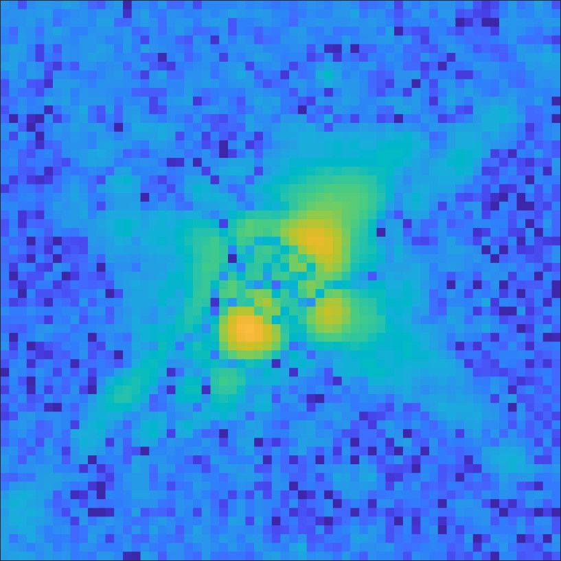
O. Beltramo-Martin et al.: Joint estimation of atmospheric and instrumental defects

Fig. 5. r0 estimates at zenith and 500 nm with respect to the GEMS/GSAOI PSF field position (left) and with respect to the PSF GALACSI/MUSE
wavelength (right).

Fig. 6. Left: histograms for the A parameter for each AO system. Right: wavefront error obtained on CANARY SCAO mode with respect to the
retrieved r0 . The solid line gives the trend in r0−5/6 .

stacking), which is 350 mas (14 pixels) for the largest spectral             a parametric OTF term. Besides, determining the wavefront from
width, the parameter estimation degrades up to 10% and goes                  a single long-exposure image suffer from strong degeneracies by
beyond the 4% threshold after 300 nm of spectral width. As a                 essence and this approach does not overcome this problem by
result, the model remains robust and reliable, even in the pres-             using a non-linear minimization algorithm to estimate the prob-
ence of such a strong beam dispersion.                                       lem solution. We distinguish two sorts of degeneracy
                                                                                  – Sign ambiguity : this occurs when trying to fit pair modes
4. Joint atmospheric, AO performance and static                              for which the PSF is not sensitive to the sign (Mugnier et al.
                                                                             2008). Therefore, we concentrate the static aberrations retrieval
   aberrations retrieval                                                     on piston, tip and tilt modes only. Moreover, we bound the solu-
The previous section illustrates that this model accurately and              tion domain between −λ/2 and λ/2 in order to overcome phase
reliably reproduces the AO residual component of the PSF.                    wrapping issues with piston modes.
Considering that the model is parsimonious (7 AO parameters                       – Local minima: two different wavefront patterns may
and 4 photometric and astrometric parameters) and the large                  produce a similar but slightly different PSF and make the PSF-
amount of pixels (10 000 for a 100 × 100 image) that the model-              fitting algorithm converge towards a local minimum of the cri-
fitting may rely on, one can attempt to retrieve more degrees of             terion. To assess how much this problem affect our algorithm,
freedom, such as static aberrations.                                         we have compared the PSF model with various conditions of
     In order to estimate the static coefficients, we replace in the         piston, tip and tilt levels in order to highlight possible combina-
criterion given in Eq. (10) h̃Static by h̃Static (µStatic ), which becomes   tions (10 000) of modes that could produce a similar PSF. From

                                                                                                                               A58, page 9 of 15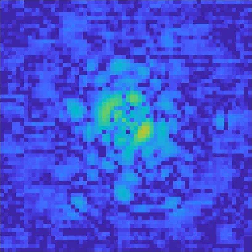
A&A 643, A58 (2020)

Fig. 7. Histograms for the β and α parameters for each system, as well as the averaged distribution.

Fig. 8. Left: average of absolute retrieved parameters with respect to the exposure time. The parameters are normalized by the value obtained
from the long-exposure PSF (60 frames). Error bars are assessed by averaging results over the SOUL/LUCI data sets. Right: average retrieved
parameters normalized by the median value over the whole span with respect to the spectral width. The envelope shows the ±4% of variations
around the median value and the spectral bandwidth is systematically centered around 700 nm. Error bars are assessed by averaging results over
the GALACSI/MUSE data sets.

a vector of aberrations, we have tested different permutations             aberration would be necessarily visible and mitigated as much as
of the elements of this vector and in 99% of cases, the rela-              possible.
tive PSF variation is larger than 1%, which is large enough to                 Henceforth, we are in a good situation to estimate piston, tip
change the structure of the PSF and retrieve the correct wave-             and tilt static modes on Keck and VLT images obtained on bright
front map, as long as the S/N is sufficient (>50). We also rely            star.
on an analysis from Gerwe et al. (2008) that shows that for a
fit of 35 Zernike polynomials on a segmented pupil, there are
                                                                           4.1. Keck cophasing error retrieval
no local minima as long as the initial guess for the static coef-
ficient remains within ±0.2λ = 330 nm rms in H-band from the               The analysis presented in this section focuses on a smaller sam-
optimal solution. We are in a situation where the static aberra-           ple of 129 Keck AO/NIRC2 data acquired in NGS mode and
tions we attempt to retrieve are already mitigated from the Keck           with a high SR (>40%) in 2013 (Ragland et al. 2016). The resid-
telescope active control (Chanan et al. 1988) and the VLT spi-             ual NCPA map was calibrated at the beginning of the night. We
ders coating (Milli et al. 2018). Consequently, the aberrations            compared model-fitting performance in three situations: (i) a fit
level we must retrieve remains sufficiently weak to mitigate the           of PSD and photometric and astrometric parameters (11 values),
presence of local minima. At a level greater than 300 nm (Keck             (ii) a fit of these parameters when including, following Eq. (2),
AO residual is 280 nm) would impact drastically the PSF and                the static aberration map calibrated at the beginning of the night
degrade the telescope science exploitation so much that this               and, (iii) a joint adjustment of the PSD, photometry/astrometry

A58, page 10 of 15
O. Beltramo-Martin et al.: Joint estimation of atmospheric and instrumental defects
Case 1 - February 2013 Case 2 - August 2013 Case 3 - September 2013
Sky
image
Model
Model
+
NCPA
Model
+
NCPA
+
Cophasing
Fig. 9. Comparison in log scale of on-sky PSFs and fitted model using the three implemented strategies. Each column correspond to a single data
sample acquired at different epochs. For each model configuration, we report both the adjusted PSF and the residual map. This figure illustrates
that the cophasing map retrieval improves drastically and consistently the residual on top of the gain brought by including the NCPA residual map.
Table 4. Median and 1-σ dispersion of SR and FWHM errors and sample we consider in the present analysis and that gathers only
mean square error obtained over the 129 H-band and high SR (>40%) high SR data for which the residual atmospheric aberrations are
Keck/NIRC2 images treated in this analysis for the three implemented weaker. This advocates for including the calibrated static aber-
strategies: (i) PSD/stellar parameters retrieval, (ii) including the resid- rations map into the model in order to mitigate this bias in the
ual NCPA map in the model, and (iii) also including the estimation of
Keck II cophasing errors.
model. From Fig. 9, we also observe that these static aberrations
manifest mainly as static speckles in the PSF and consequently
contribute marginally to shape the PSF core, which explain why
Strategy ∆ SR (pts) ∆ FWHM (mas) MSE (%) the statistics on the FWHM estimates are not influenced by the
(SR > 40%) Median Std Median Std reduction of the data sample. Moreover, the results shown in
both Fig. 9 and Table 4 highlight that the model accuracy is
(i) 1.4 1.9 −0.9 0.8 0.81 slightly improved by including the NCPA residual map in the
(ii) 1.0 1.8 −0.7 0.8 0.54 model, with still 50% improvement on the MSE. Furthermore,
(iii) 0.7 1.1 −0.5 0.4 0.32 the cophasing map retrieval allows to drastically enhance the
Notes. Systematically, accounting for the NCPA map allows us to model-fitting results, for example by up to a factor three on the
slightly reduce the biases on the estimates and diminish the MSE, MSE compared to the first scenario, as also illustrated in Fig. 9
but best model-fitting results are obtained thanks to cophasing error and Table 4. The fact that the model efficiently reproduces the
retrieval that decreases the MSE by almost a factor three. speckles observed on sky images suggests that these speckles
are mainly introduced by cophasing errors due to the telescope.
In addition, in order to further demonstrate the strength of
and the 36 piston values corresponding to each Keck pupil seg- this framework, we present in Fig. 10 the retrieved cophasing
ment (47 parameters in total), including the calibration static maps for three specific cases. The corresponding NCPA map
aberration map. used in the model is presented in Ragland et al. (2016). We
Figure 9 shows the PSFs and the residual maps produced unmistakably observe the presence of a stair mode, that intro-
from the three model-fitting strategies considered in this section duces a constant step between adjacent segment rows or columns
and obtained for three cases acquired in February, August, and and that has been already highlighted from data acquired in 2017
September, 2013. We firstly conclude that accounting for the using an alternative technique (Ragland 2018).
residual NCPA static aberrations improves the model fitting as Moreover, each of those three images was obtained with dif-
revealed by the residual map. This is also confirmed by the ferent elevation-azimuth telescope positions that are reported
results shown in Table 4 which gives the median and 1σ stan- in Table 5, which shows that the wavefront standard deviation
dard deviation of SR/FWHM estimates over the 129 data sam- value is very close to observations reported by Ragland (2018)
ples as well as the mean square error (MSE) determined from for a 45◦ telescope elevation. Also, the stair case peak-to-valley
the residual map. We firstly observe that biases and dispersion (PV) energy increases with low telescope elevation and rotates
values on the SR are larger than in Table 2, owing to the data with respect to the telescope azimuth. This observation reveals
A58, page 11 of 15A&A 643, A58 (2020)
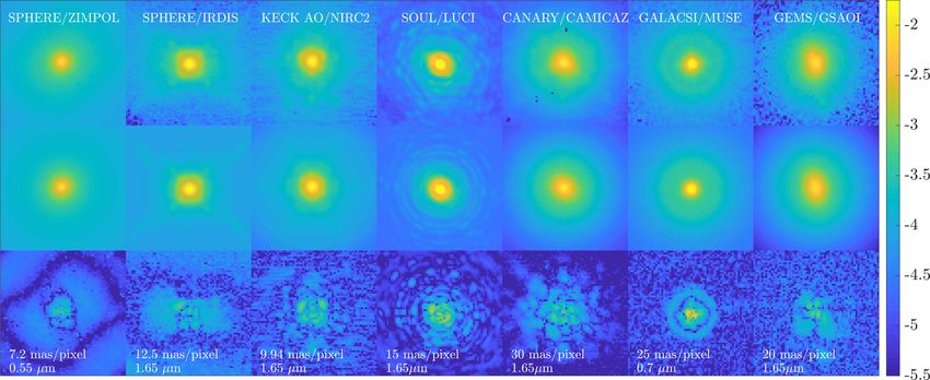
Fig. 10. Retrieved cophasing maps in nm from PSFs acquired during three different epochs in 2013. The telescope elevation and azimuth were
respectively (79,240), (85,−82) and (43,240) from left to right.
Table 5. Summary of peak-to-valley (PV) and 1-σ standard deviation Figure 11 presents the results of the two strategies imple-
of retrieved cophasing error map regarding the corresponding telescope mented in our study over three particular cases for which a strong
elevation/azimuth. LWE is observed. We observe, especially in Fig. 11, that the sole
parametrization of the PSD is not rich enough to precisely repro-
Case Elevation/Azimuth (◦ ) PV (nm) Std (nm) duce the strong asymmetry, which becomes a solved problem
thanks to the aberration parametrization we propose. Regarding
Feb. 2013 (79,240) 760 95 the estimated PSF shape and values given in Table 6, we show
Aug. 2013 (85,−82) 530 66 clear evidence that (i) describing the LWE as a combination of
Sept. 2013 (43,240) 1030 118 differential piston, tip, and tilt allows to accurately characterize
the PSF asymmetry, and (ii) accounting for this description in the
PSF model ensures that biases and dispersion on SR and FWHM
estimates are drastically mitigated. Moreover, the average MSE
a connection between the presence of this stair mode and global value over the 176 data samples is significantly diminished, that
flexure over the primary mirror that is controlled to compensate is, by a factor two. On the three cases illustrated in Fig. 11,
for the gravity effect. Deeper analyses will confirm the presence Table 7 also reports the SR and FWHM errors as well as the
of such a residual flexure on the Keck telescoped and whether or MSE obtained from the PSF-fitting. These results show clearly
not this framework now to allow us to correct for this stair mode a gain on accuracy for these particular cases for which the LWE
to generally improve the scientific exploitation of the Keck, but impact on the PSF is significant comparatively to the statistical
also future segmented telescopes. trend observed on the 176 data sets. This gain is partially miti-
Measuring the piston map from the focal-plane image is fea- gated on the statistical analysis owing to the fact that only 25% of
sible from results obtained with the present analysis, but neces- the data were noticeably contaminated by the LWE. Moreover,
sitates to have a star bright enough in the field to calibrate these the atmospheric part of the PSF model can mimic PSF asym-
aberrations. We must ensure that the shape of the primary mirror metries by modifying the ratio α x /αy in Eq. (7). Despite it leads
is controlled without the aid of a focal-plane-based technique in to an inaccurate representation of the LWE impact on the PSF,
order to achieve the best image quality regardless of the observed it permits to mitigate the SR and FWHM estimation error com-
field. We are again in a situation where we have to retrieve a few paratively to a symmetric atmospheric PSF model. As a sum-
parameters (47) from a potentially large amount of data delivered mary, fitting the twelve extra parameters to represent the LWE
by segment position sensors, temperature, pressure and humid- allows can enhance the PSF metrics estimation by a factor up to
ity sensors, atmospheric parameters near the dome and even AO five.
telemetry, which can deliver information about the piston error In order to confirm the robustness of the LWE retrieval, we
when using a pyramid WFS (Bond et al. 2018b; Schwartz et al. have compared the estimated static aberration map with ZELDA
2018). It is not easy to investigate the connection between this measurements (Vigan et al. 2019) taken during SPHERE com-
ensemble of data and the piston map, and the use of neural net-
missioning nights in 2014. The PSF-fitting was performed using
works for this purpose will be explored.
the differential tip-tilt sensor (DTTS) that delivers 32 × 32 pix-
els images (Baudoz et al. 2010; Sauvage et al. 2015) acquired
4.2. SPHERE low wind effect retrieval simultaneously with SPHERE/IRDIS using the ZELDA focal-
The analysis presented in this section focuses on 176 SPHERE/ plane mask to measure optical aberrations within the pupil-
IRDIS data obtained with good SR conditions (>40%) so as to plane. Moreover, in order to calibrate ZELDA measurements
test two different fitting strategies, namely (i) fitting the PSD and (that are in ADU) to reconstruct the phase, we followed
photometry/astrometry parameters (11 parameters) and (ii) fit- the process described by Sauvage et al. (2015) and removed
ting these latter 11, and 12 additional parameters correspond- the mean ADU value over the pupil and adjusted a multi-
ing to piston, tip, and tilt of each VLT pupil area delimited plicative factor to obtain the closest PSF possible from the
by the spiders in order to account for the LWE. According to DTTS observation as reported in Fig. 12. According to this
Sauvage et al. (2016), this description of the LWE allows the calibration, we obtained standard deviations of 173 nm rms
main impact of this effect to be reproduced, i.e., a strong PSF and 146 nm rms on the ZELDA map and the DTTS image-
asymmetry. based map,respectively, which leads to a quadratic difference
A58, page 12 of 15You can also read