Fast Dimensional Analysis for Root Cause Investigation in a Large-Scale Service Environment
←
→
Page content transcription
If your browser does not render page correctly, please read the page content below
Fast Dimensional Analysis for Root Cause Investigation in a
Large-Scale Service Environment

FRED LIN, Facebook, Inc.
KEYUR MUZUMDAR, Facebook, Inc.
NIKOLAY PAVLOVICH LAPTEV, Facebook, Inc.
MIHAI-VALENTIN CURELEA, Facebook, Inc.
SEUNGHAK LEE, Facebook, Inc.
SRIRAM SANKAR, Facebook, Inc.
Root cause analysis in a large-scale production environment is challenging due to the complexity of services
running across global data centers. Due to the distributed nature of a large-scale system, the various hardware,
software, and tooling logs are often maintained separately, making it difficult to review the logs jointly for
understanding production issues. Another challenge in reviewing the logs for identifying issues is the scale -
there could easily be millions of entities, each described by hundreds of features. In this paper we present a
fast dimensional analysis framework that automates the root cause analysis on structured logs with improved
scalability.
   We first explore item-sets, i.e. combinations of feature values, that could identify groups of samples with
sufficient support for the target failures using the Apriori algorithm and a subsequent improvement, FP-Growth.
These algorithms were designed for frequent item-set mining and association rule learning over transactional
databases. After applying them on structured logs, we select the item-sets that are most unique to the target
failures based on lift. We propose pre-processing steps with the use of a large-scale real-time database and
post-processing techniques and parallelism to further speed up the analysis and improve interpretability,
and demonstrate that such optimization is necessary for handling large-scale production datasets. We have
successfully rolled out this approach for root cause investigation purposes in a large-scale infrastructure. We
also present the setup and results from multiple production use cases in this paper.
CCS Concepts: • Information systems → Association rules; Collaborative filtering; • Computing method-
ologies → Feature selection; • Computer systems organization → Reliability; Maintainability and
maintenance; • Software and its engineering → Software maintenance tools; Software system models;
• Security and privacy → Intrusion detection systems.

Additional Key Words and Phrases: root cause analysis; anomaly detection; dimension correlation analysis;
investigation analysis; large-scale service environment
ACM Reference Format:
Fred Lin, Keyur Muzumdar, Nikolay Pavlovich Laptev, Mihai-Valentin Curelea, Seunghak Lee, and Sriram
Sankar. 2020. Fast Dimensional Analysis for Root Cause Investigation in a Large-Scale Service Environment.
Proc. ACM Meas. Anal. Comput. Syst. 4, 2, Article 31 (June 2020), 24 pages. https://doi.org/10.1145/3392149

Authors’ addresses: Fred Lin, Facebook, Inc. fanlin@fb.com; Keyur Muzumdar, Facebook, Inc. kmuzumdar@fb.com; Nikolay
Pavlovich Laptev, Facebook, Inc. nlaptev@fb.com; Mihai-Valentin Curelea, Facebook, Inc. mihaic@fb.com; Seunghak Lee,
Facebook, Inc. seunghak@fb.com; Sriram Sankar, Facebook, Inc. sriramsankar@fb.com.

Permission to make digital or hard copies of all or part of this work for personal or classroom use is granted without fee
provided that copies are not made or distributed for profit or commercial advantage and that copies bear this notice and          31
the full citation on the first page. Copyrights for components of this work owned by others than ACM must be honored.
Abstracting with credit is permitted. To copy otherwise, or republish, to post on servers or to redistribute to lists, requires
prior specific permission and/or a fee. Request permissions from permissions@acm.org.
© 2020 Association for Computing Machinery.
2476-1249/2020/6-ART31 $15.00
https://doi.org/10.1145/3392149

                               Proc. ACM Meas. Anal. Comput. Syst., Vol. 4, No. 2, Article 31. Publication date: June 2020.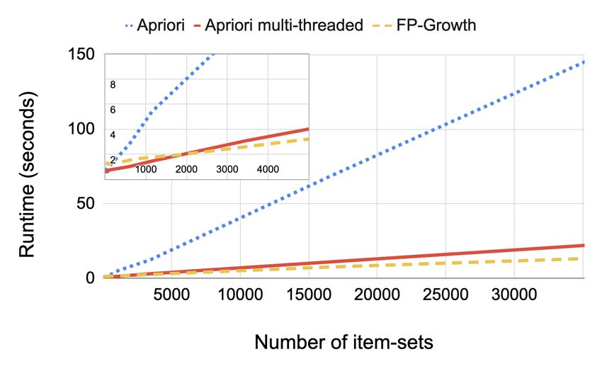
31:2                                                                                           Lin, et al.

1   INTRODUCTION
Companies running Internet services have been investing in autonomous systems for managing
large scale services, for better efficiency and scalability [12]. As some of the Internet services have
become utilities that the public relies on for transportation, communication, disaster response, etc.,
the reliability of the infrastructure is now emphasized more than before. There are various logs that
these systems record and act upon. The logs record events and configurations about the hardware,
the services, and the automated tooling, which are important in measuring the performance of the
system and tracing specific issues. Given the distributed nature and the scale of a modern service
environment, it is challenging to find and monitor patterns from the logs, because of the scale and
the complexity of the logs - each component in the system could record millions of entities that
are described by hundreds of features. An automated RCA (Root Cause Analysis) tool is therefore
needed for analyzing the logs at scale and finding strong associations to specific failure modes.
   Traditional supervised machine learning methods such as logistic regression are often not
interpretable and require manual feature engineering, making them impractical for this problem.
Castelluccio et al. proposed to use STUCCO, a tree-based algorithm for contrast set mining [4] for
analyzing software crash reports [11]. However, the pruning process in STUCCO could potentially
drop important associations, as illustrated in Section 3.7.
   In this paper, we explain how we modified the classical frequent pattern mining approach,
Apriori [2], to handle our root cause investigation use case at scale. While Apriori has been an
important algorithm historically, it suffers from a number of inefficiencies such as its runtime
and the expensive candidate generation process. The time and space complexity of the algorithm
are exponential O(2D ) where D is the total number of items, i.e. feature values, and therefore
it is practical only for datasets that can fit in memory. Furthermore, the candidate generation
process creates a large number of item-sets, i.e. combinations of feature values, and scans the
dataset multiple times leading to further performance loss. For these reasons, FP-Growth has been
introduced which significantly improves on Apriori’s efficiency.
   FP-Growth is a more efficient algorithm for frequent item-set generation [13]. Using the divide-
and-conquer strategy and a special frequent item-set data structure called FP-Tree, FP-Growth skips
the candidate generation process entirely, making the algorithm more scalable and applicable to
datasets that cannot fit in memory. As we show in the experimental results in Section 4, FP-Growth
can be 50% faster than a parallelized Apriori implementation when the number of item-sets is large.
   While FP-Growth is significantly more efficient than Apriori, some production datasets in large-
scale service environments are still too large for FP-Growth to mine all the item-sets quickly for
time-sensitive debugging. The huge amount of data could also become a blocker for memory IO or
the transfer between the database and local machines that run FP-Growth. To further speed up the
analysis, we use Scuba [1], a scalable in-memory database where many logs are stored and accessed
in real-time. As many recorded events in the production logs are identical except for the unique
identifiers such as timestamps and job IDs, we pre-aggregate the events using Scuba’s infrastructure
before querying them for the root cause analysis. The pre-aggregation step saves runtime and
memory usage significantly, and is necessary for enabling automatic RCA on production datasets
at this scale.
   The framework lets users specify irrelevant features, i.e. columns, in the structured log to be
excluded for avoiding unnecessary operations, thereby optimizing the performance. Users can
also specify the support and lift of the analysis for achieving the desired tradeoff between the
granularity of the analysis and the runtime. For example, a faster and less granular result is needed
for mission critical issues that need to remediated immediately; and more thorough results from a
slower run are useful for long-term analyses that are less sensitive to the runtime. Parallelism and

Proc. ACM Meas. Anal. Comput. Syst., Vol. 4, No. 2, Article 31. Publication date: June 2020.
Fast Dimensional Analysis for Root Cause Investigation                                                           31:3

automatic filtering of irrelevant columns are also features for achieving better efficiency, which we
discuss in Section 3.5.
   With the above optimizations, we have productionized a fast dimensional analysis framework
for the structured logs in a large-scale infrastructure. The fast dimensional analysis framework
has found various association rules based on structured logs in different applications, where the
association rules reveal hidden production issues such as anomalous behaviors in specific hardware
and software configurations, problematic kernel versions leading to failures in auto-remediations,
and abnormal tier configurations that led to an unexpectedly high number of exceptions in services.
   The rest of the paper is organized as follows: We discuss the requirements of a large-scale service
environment, the advantage of logging in a structured format, the typical RCA flow in Section 2.
We illustrate the proposed framework in Section 3. We demonstrate the experimental results in
Section 4, and the applications on large-scale production logs in Section 5. Section 6 concludes the
paper with a discussion on future work.

2     ROOT CAUSE ANALYSIS IN A LARGE-SCALE SERVICE ENVIRONMENT
2.1    Architecture of a Large-Scale Service Environment
Large scale service companies like Google, Microsoft, and Facebook have been investing in data
centers to serve globally distributed customers. These infrastructures typically have higher server-
to-administrator ratio and fault tolerance as a result of the automation that is required for running
the services at scale, and the flexibility to scale out over a large number of low-cost hardwares
instead of scaling up over a smaller set of costly machines [12]. Two important parts for keeping
such large-scale systems at high utilization and availability are resource scheduling and failure
recovery.
   Resource scheduling mainly focuses on optimizing the utilization over a large set of heterogeneous
machines with sufficient fault tolerance. Various designs of resource scheduling have been well-
documented in literature, such as Borg from Google [24], Apollo from Microsoft [9], Tupperware
from Facebook [29], Fuxi from Alibaba [32], Apache Mesos [15] and YARN [23].
   The ultimate goal for a failure recovery system is to maintain the fleet of machines at high
availability for serving applications. Timely failure detection and root cause analysis (RCA), fast and
effective remediation, and proper spare part planning are some of the keys for running the machines
at high availability. While physical repairs still need to be carried out by field engineers, most parts
in a large-scale failure recovery system have been fully automated to meet the requirements for
high availability. Examples of the failure handling systems are Autopilot from Microsoft [16] and
FBAR from Facebook [17].

2.2    Logs in a Large-Scale System
Proper logging is key to effectively optimizing and maintaining a large-scale system. In a service
environment composed of heterogeneous systems, logs come from three major sources:
      • Software - The logs populated from the services running on the servers are critical for
        debugging job failures. Job queue times and execution times are also essential for optimizing
        the scheduling system. Typically program developers have full control in how and where the
        events should be logged. Sometimes a program failure needs to be investigated together with
        the kernel messages reported on the server, e.g. out of memory or kernel panic.
      • Hardware - Hardware telemetries such as temperature, humidity, and hard drive or fan
        spinning speed, are collected through sensors in and around the machines. Hardware failures
        are logged on the server, e.g. System Event Log (SEL) and kernel messages (dmesg). The
        hardware and firmware configurations of the machine are also critical in debugging hardware

                          Proc. ACM Meas. Anal. Comput. Syst., Vol. 4, No. 2, Article 31. Publication date: June 2020.
31:4 Lin, et al.
issues, e.g. the version of the kernel and the firmwares running on different components. The
messages on the servers need to be polled at an appropriate frequency and granularity that
strikes a balance between the performance overhead on the servers and our ability to detect
the failures timely and accurately.
• Tooling - As most of the parts in the large-scale system are automated, it is important
to monitor the tools that orchestrate the operations. Schedulers would log the resource
allocations and job distribution results. Failure recovery systems would log the failure signals
and the remediation status. Historical tooling logs are important for analyzing the tooling
efficiency.
For root cause analysis in real-time, the logs are pushed to Scuba, a “fast, scalable, distributed,
in-memory database.” [1] Keeping the data in-memory, Scuba tables typically have shorter retention.
For long-term analytics, logs are archived in disk-based systems such as HDFS [8], which can be
queried by Hive [21] and Presto [22]. Some of the more detailed operational data can be fetched
from the back-end MySQL databases [19] to enrich the dataset for the analysis. The quality of the
logs has fundamental impacts on the information we can extract. We will discuss the advantages of
structured logging in Section 3.2.
2.3 Prior Root Cause Analysis Work
Root cause analysis (RCA) is a systematic process for identifying the root causes of specific events, e.g.
system failures. RCA helps pinpoint contributing factors to a problem or to an event. For example,
RCA may involve identifying a specific combination of hardware and software configurations that
are highly correlated to unsuccessful server reboots (discussed in Section 5.1), and identifying a set
of characteristics of a software job that are correlated to some types of job exceptions (discussed in
Section 5.3).
During an incident in a large-scale system, the oncall engineers typically investigate the under-
lying reason for a system failure by exploring the relevant datasets. These datasets are comprised
of tables with numerous columns and rows, and often the oncall engineers would try to find
aggregations of the rows by the column values and correlate them with the error rates. However, a
naive aggregation scales poorly due to the significant amount of the rows and distinct values in the
columns, which result in a huge amount of groups to be examined.
For automating RCA, the STUCCO algorithm has been used for contrast set mining [4, 5, 11].
Suriadi et al. [20] demonstrated an RCA approach using decision tree-based classifications from
the WEKA package [27], as well as enriching the dataset with additional features. The traditional
STUCCO algorithm, however, can miss important associations if one of the items does not meet
the pruning threshold on the χ 2 value, as explained in Section 3.7. Decision tree-based approaches,
while providing the visibility in how the features are used to construct the nodes, become harder
to tune and interpret as the number of trees grows. To ensure we capture the associations that
are relatively small in population yet strongly correlated to our target, we choose to explore all
association rules first with additional filtering based on support and lift as post-processing, as
illustrated in Section 3.6.
In association rule mining, FP-Growth [13] has become the common approach as the classical
Apriori algorithm [2] suffers from its high complexity. The state-of-the-art approaches for log-based
root cause analysis found in literature often have small-data experiments, do not handle redundant
item-sets with pre-/post-processing and fail to find root causes with small error rates relative to
successes. For example, while the authors in [30] provide a pre-processing step for pre-computing
the association matrix for speeding up association rule mining, it lacks the study of large scale
applicability and the filtering of small error classes (see Figure 5 and Section 4.2 for how the
Proc. ACM Meas. Anal. Comput. Syst., Vol. 4, No. 2, Article 31. Publication date: June 2020.Fast Dimensional Analysis for Root Cause Investigation 31:5
proposed fast dimensional analysis framework addresses these points). Similarly, the authors in
[3] provide a hybrid approach for spam detection using a Naive Bayes model with FP-Growth to
achieve better spam-detection accuracy but with a decreased interpretability because only the
prediction is provided and not the root-cause. In our use case, however, having an explainable
model is critical (see Section 4.2) and we are biased away from compromises in interpretability.
An FP-Growth implementation on Spark platform was proposed in [18], and an extension for
FP-Growth to handle negative association rules [28] was proposed in [25]. For better interpretability,
Bittmann et al. proposed to remove ubiquitous items from the item-sets using lift [6], whereas
Liu et al. used lift to further prune the mined association rules from FP-Growth [18].
For sustaining the large-scale service environment at high availability all the time, we need an
analysis framework that can handle large-scale production datasets, e.g. billions of entries per day,
and generate result in near real-time, e.g. seconds to minutes. In this paper we propose a framework
that pre-aggregates data to reduce data size by > 500X using an in-memory database [1], mines
frequent item-sets using a modified version of FP-Growth algorithm, and filters the identified
frequent item-sets using support and lift for better interpretability. We validate the framework on
multiple large-scale production datasets from a service environment, whereas the related papers
mostly demonstrate the results using relatively small synthetic datasets. We will illustrate the
details of the framework in Section 3 and compare the framework with the above-mentioned
methods in Section 4.
3 FAST DIMENSIONAL ANALYSIS
We propose an RCA framework that is based on the FP-Growth algorithm [13], with multiple
optimizations for production datasets in a large-scale service system. After querying the data, which
is pre-aggregated using Scuba’s infrastructure [1], the first step in this framework is identifying
the frequent item-sets in the target state, e.g. hardware failures or software exceptions. Item-sets are
combinations of feature values of the samples. In a structured dataset, e.g. Table 1, the columns
are considered the features of the entities, and each feature could have multiple distinct values
in the dataset. We refer to feature values as items in the context of frequent pattern mining. For
example, when analyzing hardware failures, the items could be the software configuration of the
server such as the kernel and firmware versions, as well as the hardware configuration such as
the device model of the various components. When analyzing software errors, the items could
be the memory allocation, the machines where the jobs are run, and the version of the software
package. The number of items in an item-set is called the length of the item-set. Item-sets with
greater lengths are composed of more feature values and are therefore more descriptive about the
samples.
The second step in RCA is checking the strength of the associations between item-sets and the
target states. We propose multiple pre- and post-processing steps for improving the scalability and
the interpretability of the framework in Section 3.5 and 3.6.
3.1 Metrics for Evaluating the Correlations
Three main metrics are typically considered in an RCA framework: support, confidence, and lift.
We first describe the meaning behind these metrics in the context of root cause analysis and then
describe why we picked support and lift as our main metrics to track.
Support was introduced by Agrawal, et al. in [2] as
|t ∈ D; X ⊆ t |
supp(X ) = = P(X ) (1)
|D|
where D = {t 1, t 2, ..., tn } is a database based on a set of transactions tk .
Proc. ACM Meas. Anal. Comput. Syst., Vol. 4, No. 2, Article 31. Publication date: June 2020.31:6 Lin, et al.
Support of X with respect to D refers to the portion of transactions that contain X within D. In
our RCA problem, D is equivalent to the entire structured log, while each entry is considered a
transaction t. Support has a downward closure property, which is the central idea behind Apriori
frequent item-set mining algorithm. Downward closure implies that all subsets of a frequent item-
set are also frequent. Analogously, all supersets of an infrequent item-set can be safely pruned
because they will never be frequent. The range of support is [0, 1].
When mining frequent item-sets, the frequency of an item-set is defined based on the samples in
the target failure state, so we limit the database to the transactions that cover the target failure
state Y (e.g. software job status =exception). In this context, support can therefore be formulated as
f requency(X, Y )
supp(X, Y ) = = P(X |Y ) (2)
f requency(Y )
Hereafter, we refer to supp(X ) as the support with respect to all transactions, and supp(X, Y ) as the
support with respect to the transactions covering Y .
Confidence was introduced by Agrawal et al. in [2] and is defined as
supp(X ∩ Y )
con f (X ⇒ Y ) = = P(Y |X ) (3)
supp(X )
Confidence, which ranges from 0 to 1, refers to the probability of X belonging to transactions
that also contain Y . Confidence is not downward closed and can be used in association rule mining
after frequent item-sets are mined based on support. Confidence is used for pruning item-sets
where con f (X ⇒ Y ) < γ , where γ is a minimum threshold on confidence. Using confidence is
likely to miss good predictors for Y under imbalanced distribution of labels. For example, suppose
that we have 100 failures and 1 million reference samples. If feature X exists for 100% of failures Y
but 1% of references, intuitively X should be a good predictor for Y ; however confidence will be
small (< 0.01) due to the large number of reference samples with feature X . For this reason we use
lift in our work, which we define next.
To deal with the problems in confidence, we use the lift metric (originally presented as interest)
introduced by Brin et al. [10]. Lift is defined as
con f (X ⇒ Y ) P(X ∩ Y )
li f t(X ⇒ Y ) = = (4)
supp(Y ) P(X )P(Y )
Lift measures how much more likely that X and Y would occur together relative to if they were
independent. A lift value of 1 means independence between X and Y and a value greater than 1
signifies dependence. Lift allows us to address the rare item problem, whereas using confidence we
may discard an important item-set due to its low frequency. A similar measure, called conviction,
was also defined in [10] which compares the frequency of X appearing without Y , and in that sense
it is similar to lift but conviction captures the risk of using the rule if X and Y are independent.
We use lift instead of conviction primarily due to a simpler interpretation of the result for our
customers.
3.2 Structured Data Logging
Structured logs are logs where the pieces of information in an event are dissected into a pre-defined
structure. For example, in a unstructured log we may record human-readable messages about a
server like the following:
0 : 0 0 e x p e r i e n c e d memory e r r o r
0 : 0 0 e x p e r i e n c e d memory e r r o r
0 : 0 0 e x p e r i e n c e d memory e r r o r
Proc. ACM Meas. Anal. Comput. Syst., Vol. 4, No. 2, Article 31. Publication date: June 2020.Fast Dimensional Analysis for Root Cause Investigation 31:7
0:15 r e b o o t from t o o l A
0:20 e x p e r i e n c e d memory e r r o r
0:21 t o o l B AC C y c l e d t h e machine
0:25 no d i a g n o s i s f o u n d i n t o o l A
0:26 t o o l C send to r e p a i r − undiagnosed
Table 1. Server errors and reboots logged in a structured table
timestamp memory error cpu error ... reboot undiag. diag. tool
repair repair
0:00 3 0 0 0 0 NULL
0:15 0 0 1 0 0 A
0:20 1 0 0 0 0 NULL
0:21 0 0 1 0 0 B
0:26 0 0 1 1 0 C
There are a few major drawbacks in this example log. First, the same message appears multiple
times, which can be aggregated and described in a more succinct way to save space. Second, tool
A and tool B both write to this log, but in very different formats. Tool A and B both restarted the
server by turning the power off and on, but tool A logs it as “reboot”, while tool B, developed by
another group of engineers from a different background, logs it as a verb “AC Cycle”. This could
even happen to the same word, for example, “no diagnosis” and “undiagnosed” in the last two
messages mean the same condition, but would impose huge difficulty when one tries to parse this
log and count the events with regular expressions.
With a pre-defined structure, i.e. a list of fields to put the information in, structured logging
requires a canonical way to log events. For example, in a structured table, the messages above can
be logged in the format shown in Table 1.
In this conversion, engineers could decide not to log “no diagnosis found in tool A” in the
structured table because it does not fit in the pre-defined structure. The structure of the table is
flexible and can be tailored to the downstream application, for example, instead of having multiple
columns for memory error, cpu error, etc., we can use one “error” column and choose a value from
a pre-defined list such as memory, cpu, etc., to represent the same information.
In addition to removing the ambiguity in the logs, enforcing structured logging through a single
API also helps developers use and improve the existing architecture of the program, instead of
adding ad-hoc functionalities for edge cases, which introduces unnecessary complexity that makes
the code base much harder to maintain. In this example, if there is only one API for logging a reboot,
developers from tool A and B would likely reuse or improve a common reboot service instead of
rebooting the servers in their own code bases. A common reboot service would be much easier to
maintain and likely have a better-designed flow to handle reboots in different scenarios.
3.3 Frequent Pattern Mining and Filtering
Our proposed RCA framework involves two steps: frequent pattern 1) mining and 2) filtering.
Frequent patterns in the dataset are first reported, followed by an evaluation on how strongly each
frequent pattern correlates to the target failures.
In frequent pattern mining, each item should be a binary variable representing whether a
characteristic exists. In a production structured dataset, however, a column would usually represent
one feature, which could have multiple distinct values, one for each entity. Therefore the structured
Proc. ACM Meas. Anal. Comput. Syst., Vol. 4, No. 2, Article 31. Publication date: June 2020.31:8 Lin, et al.
log needs to first be transformed into a schema that fits the frequent pattern mining formulation.
The transformation is done by applying one-hot encoding [14] on each of the columns in the
structured table. For a column in the structured table f , which has k possible values in a dataset,
one-hot encoding "explodes" the schema and generate k columns {f 0 , f 1 , ..., fk −1 }, each contains a
binary value of whether the entity satisfies f = fk .
Apriori is a classical algorithm that is designed to identify frequent item-sets. As illustrated
in Algorithm 1, starting from frequent items, i.e. item-sets at length=1, the algorithm generates
candidate item-sets by adding one item at a time, known as the candidate generation process. At
each length k, candidate generation is done and all the candidate item-sets are scanned to increment
the count of their occurrences. Then the item-sets that meet the min-support threshold are kept and
returned as the frequent item-set L K . We add a practical constraint max-length on the maximum
length of the item-set that we are interested in. The limit on max-length stops the algorithm from
exploring item-sets that are too descriptive and specific to the samples, which are typically less
useful in production investigation.
3.4 Architecture of a Large-Scale Service Environment
Algorithm 1: Apriori Algorithm
let Ck be the candidate item-sets at length= k
let Lk be the frequent item-sets at length= k
L 1 = frequent items
k=1
while Lk , ϕ and k ≤ max_lenдth do
Ck +1 = candidate item-sets generated from Lk
foreach transaction t in database do
foreach item-set c covered by t do
increment the count of c
end
end
Lk +1 = item-sets in Ck +1 that meet min-support
k++
end
return ∪Lk
By generating a large set of candidates and scanning through the database many times, Apriori
suffers from an exponential run time and memory complexity (O(2D )), making it impractical for
many production datasets. The FP-Growth algorithm, based on a special data structure FP-Tree, was
introduced to deal with performance issues by leveraging a data structure that allows to bypass the
expensive candidate generation step [13]. FP-Growth uses divide-and-conquer by mining short
patterns recursively and then combining them into longer item-sets.
Frequent item-set mining through FP-Growth is done in two phases: FP-Tree construction
and item-set generation. Algorithm 2 shows the process of FP-Tree construction. The FP-Tree
construction process takes two inputs: 1) the set of samples in the target failure state (equivalent
to a transaction database in classical frequent pattern mining literature), and 2) a min-support
threshold, based on which a pattern is classified as frequent or not. Each node in the tree consists
of three fields, item-name, count, and node-link. item-name stores the item that the node represents,
Proc. ACM Meas. Anal. Comput. Syst., Vol. 4, No. 2, Article 31. Publication date: June 2020.Fast Dimensional Analysis for Root Cause Investigation 31:9
count represents the number of transactions covered by the portion of the path reaching the node,
and node-link links to the next node with the same item-name. The FP-tree is constructed in two
scans of the dataset. The first scan finds the frequent items and sort them, and the second scan
constructs the tree.
Algorithm 2: FP-Tree Construction
Scan data and find frequent items
Order frequent items in decreasing order with respect to support, F
Create root node T , labeled as NULL
foreach transaction t in database do
foreach frequent item p in F do
if T has a child N such that N .item-set=p.item-set then
|N | + +
end
else
Create N , link parent-link to T , and set N .count = 1
Link N ’s node-link to nodes with the same item-name
end
end
end
Algorithm 3 illustrates the process for generating the frequent item-sets, based on the lemmas
and properties Han et al. proposed in [13]. A conditional pattern base is a sub-database which
contains the set of frequent items co-occurring with the suffix pattern. The process is initiated by
calling F P-Growth(T ree, NU LL), then recursively building the conditional FP-Trees.
Algorithm 3: Frequent Item-set Generation
Function FB-Growth(T ree, α):
if T ree contains a single path P then
foreach combination β of nodes in path P do
Generate pattern β ∪ α with support = min support of nodes in β
end
end
else
foreach α i in tree do
Generate pattern β = α i ∪ α with support = α i .support
Construct β’s conditional pattern base and β’s conditional FP-tree T β
if T β , ϕ then
call FB-Growth(T β , β)
end
end
end
After finding the frequent item-sets in the dataset, we examine how strongly the item-sets can
differentiate positive (e.g. failed hardware/jobs) samples from the negative ones. We use lift, defined
Proc. ACM Meas. Anal. Comput. Syst., Vol. 4, No. 2, Article 31. Publication date: June 2020.31:10 Lin, et al.
in Section 3.1, to filter out item-sets that are frequent in the failure state but not particularly useful
in deciding if a sample will fail. For example, an item-set can be frequent in both non-failure and
failure states, and the evaluation based on lift would help us remove this item-set from the output
because it is not very useful in deciding whether samples in that item-set would fail or not.
3.5 Pre- and Post-Processing for Performance Optimization
We incorporated multiple optimizations as pre- and post-processing to scale the RCA framework
for accommodating near real-time investigations, which are important in responding to urgent
system issues quickly. Many entities in a production log are identical, except the columns that are
unique identifiers of the entities such as the timestamps, hostnames, or job IDs. Utilizing Scuba’s
scalable infrastructure [1], we query pre-aggregated data which are already grouped by the distinct
combinations of column values, with an additional weight column that records the count of the
identical entities. To handle this compact representation of the dataset, we modified the algorithms
to account for the weights. This pre-aggregation significantly reduces the amount of data that we
need to process in memory and would reduce the runtime of our production analyses by > 100X .
Columns that are unique identifiers about the entities need to be excluded before the Scuba
query. The aggregation in Scuba is only meaningful after excluding these columns, otherwise the
aggregation would return one entity per row due to the distinct values per entity. The framework
allows users to specify columns to be excluded in the dataset, as well as automatically checks
to exclude columns with the number of distinct values > D portion of the number of samples.
Empirically, we use D = 2% in one of our applications, and the proper setting of D highly depends
on the nature of the dataset.
Adding multithreading support to the algorithm further improves Apriori’s performance, as the
algorithm generates a large number of combinations and test them against the data. By testing
these combinations in parallel, we can scale up with the number of available cores. However, we
found that FP-Growth outperforms Apriori even when Apriori is optimized with multithreading.
3.6 Interpretability Optimization
In production datasets, it is common that there exist a large number of distinct items, and the
lengths of the findings are typically much smaller than the number of the one-hot encoded feature
columns (as discussed in Section 3.3). As a result, there can be multiple findings describing the
same group of samples. To improve the quality of the result, we implemented two filtering criteria
for removing uninteresting results as described below:
Filter 1: An item-set T is dropped if there exists a proper subset U , (U ⊂ T ) such that li f t(U ) ∗
Hlif t ≥ li f t(T ), where Hl if t ≥ 1
If there exist shorter rules with similar or higher lift, longer rules are pruned because they
are less interesting. Hl if t is a multiplier that can be tuned based on the nature of the dataset, to
remove more longer rules, as it makes the condition easier to be satisfied. This filter addresses the
ubiquitous items discussed in [6]. As there exists a shorter rule with similar or higher lift, the one
containing the ubiquitous item will be filtered out. Consider two rules:
{ k e r n e l A , s e r v e r t y p e B } => f a i l u r e Y w i t h l i f t 5
{ k e r n e l A , s e r v e r t y p e B , d a t a c e n t e r C } => f a i l u r e Y w i t h l i f t 1.5
Proc. ACM Meas. Anal. Comput. Syst., Vol. 4, No. 2, Article 31. Publication date: June 2020.Fast Dimensional Analysis for Root Cause Investigation 31:11
It is likely that describing the server and kernel interaction is more significant than filtering by
datacenter, therefore the second rule is pruned, even though the lift values from both rules meet
our threshold on the minimum lift.
Filter 2: An item-set T is dropped if there exists a proper superset S, (S ⊃ T ) such that supp(S) ∗
Hsupp ≥ supp(T ) and li f t(S) > li f t(T ) ∗ Hl if t , where Hsupp ≥ 1 and Hlif t ≥ 1
If a rule has a superset which describes a similar number of samples, i.e. similar support, and
the superset’s lift is higher, the rule will be dropped as the superset is a more powerful rule that
describes most or all of the samples. Similarly, Hsupp is applied to loosen the comparison criteria
for support, and Hl if t is applied to ensure that the lift difference is sufficiently large based on the
use case. For example, consider two rules:
{ d a t a c e n t e r A } => f a i l u r e Y w i t h s u p p o r t 0 . 8 and l i f t 2
{ d a t a c e n t e r A , c l u s t e r B , r a c k C } => f a i l u r e Y w i t h s u p p o r t 0 . 7 8
and l i f t 6
In this scenario, almost all of the samples in datacenter A are also in cluster B and rack C. When
trying to understand the root cause of the failures, the longer item-set with a higher lift and a
similar support is more informative, so we keep it and remove the shorter item-set.
In summary, we prefer to keep shorter item-sets when the lift values are similar. When a longer
item-set’s lift value is significantly higher than that of a subset, and the support values are similar,
we keep the longer item-set.
3.7 The Proposed Framework
Our final implementation incorporating the above-mentioned improvements is illustrated in Figure 1.
Utilizing Scuba’s scalable, in-memory infrastructure [1], we query data that is aggregated by the
group-by operation based on the distinct value combinations in a set of columns. The aggregation
is done excluding columns that the users specify as not useful, and columns that our check finds to
have too many distinct values to satisfy a practical minimum support threshold. One-hot encoding
is then applied to the queried data for converting the column-value pairs to Boolean columns, or
items. We apply frequent pattern mining techniques such as Apriori and FP-Growth on the dataset
to identify frequent item-sets, which are then filtered by lift because in RCA we are only interested
in item-sets that are useful in separating the target labels, e.g. specific failure states, from the rest
of the label values, e.g. successful software task states. Finally the filtering criteria in Section 3.6
are applied to further condense the report for better interpretability.
In our framework we choose to filter the association rules by lift and support after the rules are
mined with FP-Growth, instead of pruning the association rules during the tree construction as
the STUCCO algorithm does in a contrast set mining problem [4, 5, 11]. This helps us find more
granular item-sets with high lift that would otherwise be missed. For example, if association rule
{A, B} ⇒ Y has a high lift (or the χ 2 statistic as in STUCCO), but both {A} ⇒ Y and {B} ⇒ Y
have lift (or χ 2 statistic) values below the pruning threshold, {A, B} ⇒ Y would not be found if
we prune the tree based on both support and lift (or χ 2 statistic) as STUCCO does. In STUCCO,
every node needs to be significant based on chi-square tests and large based on support for it to
have child nodes [5]. On the other hand, as FP-Growth mines frequent item-sets only based on
support, as long as {A} ⇒ Y , {B} ⇒ Y , and {A, B} ⇒ Y have enough support, they would all be
reported as frequent item-sets. Then {A} ⇒ Y and {B} ⇒ Y will be filtered out due to low lift
while {A, B} ⇒ Y will be reported in the final result.
Proc. ACM Meas. Anal. Comput. Syst., Vol. 4, No. 2, Article 31. Publication date: June 2020.31:12 Lin, et al.
User-Specified Filters
Variability-Based Filters
Query and Dedup (Scuba)
One-Hot Encoding
Frequent Pattern Mining (Apriori / FP-Growth)
Initial Pattern Filtering Using Lift
Further Filtering for Interpretability
Fig. 1. The proposed framework for the Fast Dimensional Analysis.
4 EXPERIMENTAL RESULTS
In this section we present the optimization result for runtime and interpretability, based on their
relationships with the min-support and max-length parameters during item-set mining, as well as
the min-lift during item-set filtering. We experimented on two production datasets:
• Anomalous Server Events
This is a dataset about anomalous behaviors (e.g. rebooted servers not coming back online)
on some hardware and software configurations (more details can be found in Section 5.1).
We compiled the dataset with millions of events, each described by 20 features. The features
expand to about 1500 distinct items after one-hot encoding, with tens of thousands of distinct
valid item-sets. Approximately 10% of the data are positive samples, i.e. anomalous behaviors.
For simplicity we refer to this dataset as ASE in the rest of the paper.
• Service Requests
This is a dataset that logs the requests between services in a large-scale system. Each request
is logged with information such as the source and destination, allocated resource, service
specifications, and authentication (more details can be found in Section 5.2). For experimenta-
tion, we compiled a dataset that contains millions of requests, each described by 50 features.
The features expand to about 500 distinct items after one-hot encoding, with 7000 distinct
valid item-sets. Approximately 0.5% of the data are positive samples. For simplicity we refer
to this dataset as SR in the rest of the paper.
As the datasets are different by an order of magnitude in terms of the proportion of positive
samples, we expect our range of lift to vary considerably. Additionally, the ASE dataset contains
almost 5X the number of distinct feature values as the SR dataset does, which would affect the
count and length of item-sets mined with respect to min-support. We demonstrate the results based
on these two datasets with the different characteristics below.
4.1 Performance Improvement
4.1.1 Data Pre-Aggregation. As described in Section 3.5, many events in production logs are
identical, except for the unique identifiers such as job IDs, timestamps, and hostnames. The pre-
aggregation of the data could effectively reduce the size of the ASE dataset by 200X and the SR
Proc. ACM Meas. Anal. Comput. Syst., Vol. 4, No. 2, Article 31. Publication date: June 2020.Fast Dimensional Analysis for Root Cause Investigation 31:13
dataset by 500X , which significantly improves both the data preparation time and the execution
time of the FP-Growth algorithm.
Table 2 shows the runtime needed for querying the data and grouping the entries with and
without the pre-aggregation using Scuba’s infrastructure. Without the pre-aggregation step in
Scuba, the data is queried from Scuba and grouped in memory before our framework consumes it.
Without pre-aggregation, the large amount of data that is transferred has a significant performance
impact on the query time. Overall the data preparation time is improved by 10X and 18X for the
ASE and SR datasets.
Table 2. Data preparation time with and without pre-aggregation in Scuba (in seconds)
Scuba query time Grouping time Total time
(including pre-agg. time) (in memory)
ASE (without pre-agg.) 3.00 0.94 3.94
ASE (with pre-agg.) 0.39 - 0.39
SR (without pre-agg.) 3.35 0.71 4.06
SR (with pre-agg.) 0.22 - 0.22
After the data is grouped, we execute our modified FP-Growth algorithm which takes the count
of samples per unique item-set, as a weight for additional input. The details of the modification is
discussed in Section 3.5. The additional weight value is used in calculating the support and lift of
an item-set, and has negligible overhead on the algorithm’s runtime. Effectively, this means the
algorithm now only need to handle 200X and 500X fewer samples from the ASE and SR datasets.
Hence, the pre-aggregation of the data is critical for enabling automatic RCA at this scale in near
real-time. This is one of the major features of this paper, as most of the prior works mentioned in
Section 2.3 did not incorporate any optimization using a production data infrastructure, and could
not handle large-scale datasets in near real-time.
4.1.2 Optimizing for Number of Item-Sets. Item-set generation is the biggest factor in runtime
of the proposed framework. We first examine the relationship between the number of reported
frequent item-sets and min-support and max-length in Figure 2. Note that the vertical axes are in
log scale.
In Figure 2a, based on the anomalous server event (ASE) dataset, we see an exponential decrease
in the number of item-sets as we increase min-support. Theoretically, the number of candidate
Ímax −l enдt h number of items
item-sets is bounded by k =1 k . In practice, however, the number of candidates
is much lower because many items are mutually exclusive, i.e. some item-sets would never exist in
production. The number of item-sets based on the three max-length values converge to within an
order of magnitude when min-support is around 0.4, meaning a greater proportion of item-sets
with support greater than 0.4 can be covered by item-sets at length 3.
Checking the convergence point helps us decide the proper max-length, given a desired min-
support. For example, in a use case where the goal is to immediately root cause a major issue in
production, we would be interested in item-sets with higher supports. In the ASE example, if our
desired min-support is greater than the convergence point in Figure 2a, say 0.95, we only need
to run the analysis with max-length set to 3, to avoid unnecessary computations for optimized
performance.
Proc. ACM Meas. Anal. Comput. Syst., Vol. 4, No. 2, Article 31. Publication date: June 2020.31:14 Lin, et al.
Max-length 3 Max-length 4 Max-length 5
Number of item-sets
10000
(log-scale)
1000
100
10
0.2 0.4 0.6 0.8 1
Min-support
(a) ASE dataset
Max-length 3 Max-length 4 Max-length 5
1000000
Number of item-sets
(log-scale)
100000
10000
1000
0.2 0.4 0.6 0.8 1
Min-support
(b) SR dataset
Fig. 2. Relationship between number of mined item-sets and min-support and max-length.
On the other hand, if the goal is to thoroughly explore the root causes for smaller groups,
with less concerns about the runtime, we could set the min-support to a smaller value such as
0.4. In this case, max-length should be set sufficiently high so that second filter discussed in
Section 3.6 can be effective to improve interpretability. For example, if a rule of interest is described
by {A, B, C, D, E} ⇒ Y , but max-length is smaller than 5, up to max −l5enдth item-sets could be
generated to represent this rule at the same support, whereas if max-length is set to 5, the exact
rule of interest would be created and the rest item-sets with smaller lengths would be dropped by
the second filter in Section 3.6, as long as the rule of interest has a higher lift.
The same trends are observed in Figure 2b for the service request (SR) dataset when increasing
min-support or max-length, but there does not exist a clear convergence point. Additionally, the
number of item-sets are non-zero when min-support is as high as 1, implying there are multiple
item-sets with support being 1 at the different max-lengths. In practice, these item-sets with
support being 1 often could be represented by more specific item-sets, i.e. supersets, and therefore
could be filtered out by the filters in Section 3.6 if the supersets have higher lift. Figure 2a and
Figure 2b demonstrate that the relationship between the number of mined item-sets and min-
support is dataset-dependent, and the convergence point of different max-lengths determined by
the complexity of the datasets.
Proc. ACM Meas. Anal. Comput. Syst., Vol. 4, No. 2, Article 31. Publication date: June 2020.Fast Dimensional Analysis for Root Cause Investigation 31:15
4.1.3 Runtime Improvement. An advantage of Apriori is that it is easily parallelizable, by splitting
up the candidate generation at each length. The optimal parallelism level depends on the number
of candidates, since each thread induces additional overhead. Figure 3 illustrates the runtime of
Apriori at different levels of parallelism, based on the ASE dataset. The runtime is reported based
on a machine with approximately 50 GB memory and 25 processors. As shown in the figure, a
9-thread parallelism resulted in the shortest runtime due to a better balance between the runtime
reduction from parallel processing and the runtime increase from parallelization overheads. Every
parallelism level up to 24 threads outperforms the single-threaded execution.
1 5 9 24
200
Runtime (seconds)
150
100
50
0
0 0 0 0 0 0
00 00 00 00 00 00
10 20 30 40 50 60
Number of item-sets
Fig. 3. Runtime of Apriori at different thread counts, based on the ASE dataset.
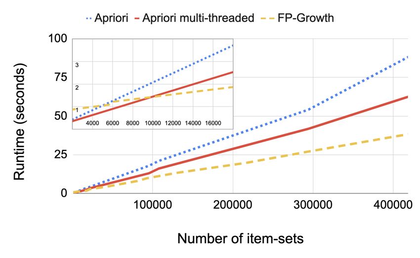
In Figure 4, we compare the runtime of Apriori [2], parallelized Apriori, and FP-Growth [3, 6,
13, 18, 25], at different number of item-sets. Note that the 9-thread configuration from Figure 3 is
used as the multi-threaded case here. It is clear that FP-Growth outperforms single-threaded and
multi-threaded Apriori, except when the number of item-sets is small, as the overhead of setting
up the FP-Growth algorithm (see Section 3.3) is larger than the benefit of not running Apriori’s
candidate generation step. However, in our experiments, FP-Growth is never slower for more than
1 second. The runtime difference could become more significant when this RCA framework is
deployed on a resource-limited platform, such as an embedded system. In Figure 4b, we see that for
the SR dataset, Apriori can be faster when the number of item-sets is smaller than 10000, which
happens when max-length < 4 or (max-length = 4 and min-support ≥ 0.8). For the ASE dataset,
multi-threaded Apriori is faster than FP-Growth when the number of item-sets is smaller than
2000, which happens when min-support ≥ 0.4. For a given dataset, running an initial scan over the
algorithms, lengths, and supports can help optimize the choice of algorithm and min-support.
4.2 Interpretability Improvement
As described in Section 3.1, lift is used when filtering the mined frequent item-sets based on their
ability in deciding whether a sample satisfying the item-set would be positive (e.g. be in the target
failure states). Figure 5a shows the number of association rules given different min-lift thresholds
on the ASE dataset, when min-support is set to 0.4 and max-length is set to 5.
There is a clear drop after min-lift = 1, which indicates rules that are stronger than randomness.
The number of association rules remains constantly at 6 when min-lift is between 2.7 and 7.9. In
practice, we can set the min-lift to anywhere between 2.7 and 7.9 to output these 6 rules as the
potential root causes, as they are the relatively stronger and more stable rules in the dataset. The
Proc. ACM Meas. Anal. Comput. Syst., Vol. 4, No. 2, Article 31. Publication date: June 2020.31:16 Lin, et al.
(a) ASE dataset
(b) SR dataset
Fig. 4. Analysis runtime vs. number of item-sets.
triangle marker indicates when an example actionable insight appears at the highest min-lift value
(more discussions in Section 5.1).
Figure 5b shows the same analysis based on the SR dataset, with min-support set to 0.5 and
max-length set to 5. The number of association rules reported drops significantly in several steps.
This is because there does not exist a clear convergence point for different max-length values, as
seen in Figure 2b, many of the reported association rules actually describe the same underlying
rules, and therefore are filtered out together as min-lift increases. The triangle marker shows when
an example actionable insight appears at the highest min-lift value (more discussions in Section 5.2).
Compared to the ASE dataset, the lift is much larger in the SR dataset.
To understand the larger trend across all association rules in the ASE dataset, we consider more
item-sets by lowering min-support to 0.1. An exponentially decreasing trend can be observed in
Figure 6. For reference, we kept the same triangle marker at min-lift = 7.9, representing a highly
Proc. ACM Meas. Anal. Comput. Syst., Vol. 4, No. 2, Article 31. Publication date: June 2020.Fast Dimensional Analysis for Root Cause Investigation 31:17
80
Number of association rules
60
40
20
0
2 4 6 8
Min-lift
(a) ASE dataset
40
Number of association rules
30
20
10
0
5000 10000 15000 20000 25000
Min-lift
(b) SR dataset
Fig. 5. Number of reported association rules vs. min-lift threshold. The triangle marks when a target rule
appears in the use cases discussed in Section 5.
actionable insight confirmed by service engineers. This graph also illustrates the importance of
setting a sufficiently high min-support to reduce noise. When using min-support 0.4 derived from
Figure 5a, we have six rules above lift 7 compared to 1200 for min-support 0.1.
With the two post-processing filters described in Section 3.6, at max-length = 5 and min-lift = 1,
we kept only 2% and 26% of the mined rules from the ASE dataset when min-support is 0.1 and 0.4,
while we kept only 0.4% and 1% of the mined rules from the SR dataset when min-support is 0.1
and 0.5. The post-processing reduces the number of mined association rules significantly without
losing the important root cause information, which makes the output report much easier for human
to examine and debug quickly. While the work in [18] integrates the FP-Growth algorithm with the
Spark platform for processing large datasets and uses lift for pruning mined item-sets, it did not
provide well-formulated post-processing steps or characterize the relationship between min-lift
and the mined item-sets.
4.3 Lessons Learned
While the results presented in this paper demonstrate effective RCA, in practice, the relationships
between these parameters are highly dependent on the nature of the datasets. Therefore we present
methods for optimizing the performance and interpretability. First of all, min-support is a variable
Proc. ACM Meas. Anal. Comput. Syst., Vol. 4, No. 2, Article 31. Publication date: June 2020.31:18 Lin, et al.
2000
Number of association rules
1500
1000
500
0
50 100 150 200
Min-lift
Fig. 6. Number of association rules at different min-lift thresholds based on the ASE dataset, when min-
support is set to 0.1. The triangle marks when a target rule appears in the use case discussed in Section 5.
that controls how granular the reported rules would be. In a real-time analysis or debug, a lower
max-length can be set to reduce runtime, and a higher min-support can be applied to report only
the most dominant issues in the dataset. In a more thorough analysis that is less time-sensitive, a
higher max-length can be applied to generate a set of rules that are overall more descriptive, based
on the filtering criteria in Section 3.6.
If there exists a clear convergence point given different max-lengths, a lower max-length should
be used to avoid unnecessary computation. If the RCA application is very sensitive to runtime and
the number of item-sets is small, one could first run the analysis similar to the one presented in
Figure 4 and use multi-threaded Apriori in the region where it outperforms FP-Growth.
The advantage of support and lift is that they are very interpretable and intuitive metrics that
any service engineer can adjust. One intuition behind the lift value is to make sure we handle the
edge case where a label value, e.g. specific failure states, has attribution X , and no other label values
has attribution X .
5 USE CASE STUDY
The method discussed in this paper has been productionized in multiple hardware, software, and
tooling applications in our large-scale service infrastructure. Deployment of this framework allows
for fast root cause analysis as well as automatic alerting on new correlations in the datasets, which
may indicate unexpected changes in the systems. In this section we present some of the applications
and the insights (after sanitizing the data) that were extracted by the proposed framework.
5.1 Anomalous Hardware and Software Configurations
In a large infrastructure, maintenance activities are constantly undertaken by the management
system - for instance, we might need to provision new services on a particular server platform.
In such scenarios, there might be reasons to reboot servers. One root cause example here is to
detect whether all servers have booted back up after a maintenance event. Using our framework,
we found a group of servers that failed to come back online as compared to the rest of the cohorts.
Without our proposed root cause analysis, the issue was isolated to a combination of 1) a specific
firmware version in one component, 2) a particular component model from a manufacturer, and 3)
a particular server model, by experienced experts after hours of investigation.
Proc. ACM Meas. Anal. Comput. Syst., Vol. 4, No. 2, Article 31. Publication date: June 2020.Fast Dimensional Analysis for Root Cause Investigation 31:19
To emulate how the proposed fast dimensional analysis could have helped with the root cause
analysis, we looked at the historical data and labeled the servers by whether the reboots were suc-
cessful on them. For example, since the servers that stayed offline is our target of the investigation,
we labeled them as positive, and the rest where the reboots were successful as negative. Then we
compiled a dataset that joins the labels with about 20 attributes of the servers, such as the server
model, the type of services the servers were running, firmware and kernel versions, component
vendors/models/firmware versions. These attributes are where we expect to find potential cor-
relations for distinguishing between the positive and negative samples. This is the first dataset
presented in the experimental results in Section 4, i.e. the anomalous server event (ASE) dataset.
With this dataset, the fast dimensional analysis framework identified the correlation based on
exactly the three attributes in 2 seconds. The lift value where this target association rule shows up
is marked by the triangle in Figure 5a. Through our methodology, we significantly reduced the
investigation time from hours to seconds. Note that in this case, there were multiple combinations
of feature values that correlate to the positive samples equally. For example, a combination of
{firmware version, component model, server model} would show the same support and lift as a
combination of {storage interface, component model, CPU model}, on this specific dataset. Purely
based on this dataset, the algorithm would not be able to tell which combination is more useful
given the type of failures. Further analysis can determine the most effective way to reduce the
number of combinations reported, potentially based on the past reports. The reported combinations
already provides strong correlations to the failures and an engineer with some experience can
quickly conclude the issue from the report.
5.2 Anomalous Service Interactions
All the communications between backend services in our large-scale system are logged. This infor-
mation is used to investigate errors in the communication among services, based on characteristics
such as latency, timeouts, requests, responses, traffic (volume, source and destination regions). This
is the second dataset, i.e. the service request (SR) dataset presented in the experimental results in
Section 4.
The naive investigation where engineers aggregate the various parameters through a group-by
operation does not scale, as there are too many distinct combinations of the column values. We
deployed the fast dimensional analysis framework to analyze two types of anomalous service
interactions: errors and latency. The analysis quickly identified attributes of service communication
that would lead to different types of errors and reported the findings. In one example for a globally
distributed service, it was reported that the errors were caused only for communications between
two specific geographical locations. This prompted engineers to investigate in this direction and
fix the issue timely. An actionable insight based on {service type, build version} ⇒ failure is marked
by the triangle in Figure 5.
Latency is not discrete when compared to errors, hence we need to first bucketize latency values
into a finite number of intervals, e.g. acceptable and non-acceptable latencies. The framework then
identifies the combinations of features where requests have non-acceptable latencies. By tuning
the bucketing threshold we obtained insightful correlations based on the features of the service
requests, which are used to optimize the performance of the systems.
5.3 Failed Auto-Remediations
We deployed the fast dimensional analysis framework on the logs from an auto-remediation
system [16, 17, 24] to quickly identify attributes of the remediation jobs that would lead to different
types of exceptions, and report the correlations to a visualization dashboard that engineers use
everyday for monitoring system health. For analyzing the correlations in auto-remediation jobs,
Proc. ACM Meas. Anal. Comput. Syst., Vol. 4, No. 2, Article 31. Publication date: June 2020.You can also read