SCOPE 2.0: a model to simulate vegetated land surface fluxes and satellite signals - GMD
←
→
Page content transcription
If your browser does not render page correctly, please read the page content below
Geosci. Model Dev., 14, 4697–4712, 2021
https://doi.org/10.5194/gmd-14-4697-2021
© Author(s) 2021. This work is distributed under
the Creative Commons Attribution 4.0 License.

SCOPE 2.0: a model to simulate vegetated land
surface fluxes and satellite signals
Peiqi Yang, Egor Prikaziuk, Wout Verhoef, and Christiaan van der Tol
University of Twente, Faculty ITC, P.O. Box 217, 7500 AE Enschede, the Netherlands

Correspondence: Christiaan van der Tol (c.vandertol@utwente.nl)

Received: 31 July 2020 – Discussion started: 28 October 2020
Revised: 23 May 2021 – Accepted: 27 June 2021 – Published: 29 July 2021

Abstract. The Soil Canopy Observation of Photosynthesis            1   Introduction
and Energy fluxes (SCOPE) model aims at linking satellite
observations in the visible, infrared, and thermal domains         Vegetation, as a dynamic component of the Earth system,
with land surface processes in a physically based manner,          affects the climate via its influence on the exchange of en-
and quantifying the microclimate in vegetation canopies. It        ergy and matter between the land surface and the atmosphere.
simulates radiative transfer in the soil, leaves, and vegetation   Quantification of this exchange is relevant for a wide range
canopies, as well as photosynthesis and non-radiative heat         of applications including weather prediction, climate projec-
dissipation through convection and mechanical turbulence.          tions, agriculture, and ecological and hydrological studies.
Since the first publication 12 years ago, SCOPE has been ap-          Process-based terrestrial ecosystem models describe the
plied in remote sensing studies of solar-induced chlorophyll       exchange of water, carbon, energy among soil, vegetation,
fluorescence (SIF), energy balance fluxes, gross primary pro-      and atmosphere in a mechanistic way. A number of models
duction (GPP), and directional thermal signals. Here, we           have been developed since 1970s, such as the comprehensive
present a thoroughly revised version, SCOPE 2.0, which fea-        plant–environment model Cupid (Norman, 1979), the Sim-
tures a number of new elements: (1) it enables the definition      ple Biosphere model (SiB, Sellers et al., 1986), the Boreal
of layers consisting of leaves with different properties, thus     Ecosystem Productivity Simulator (BEPS, Liu et al., 1997),
enabling the simulation of vegetation with an understorey          the Biosphere Energy Transfer Hydrology model (BETHY,
or with a vertical gradient in leaf chlorophyll concentration;     Rayner et al., 2005), and the models in the Trends in
(2) it enables the simulation of soil reflectance; (3) it in-      Net Land-Atmosphere Carbon Exchange project (TRENDY,
cludes the simulation of leaf and canopy reflectance changes       Sitch et al., 2008). Proper representation of the land surface
induced by the xanthophyll cycle; and (4) the computation          and the response of net CO2 exchange to changes in envi-
speed has been reduced by 90 % compared to earlier ver-            ronmental conditions (e.g. temperature and precipitation) is
sions due to a fundamental optimization of the model. These        crucial for accurately modelling future climate and climate–
new features improve the capability of the model to repre-         carbon cycle feedbacks. Terrestrial ecosystem models con-
sent complex canopies and to explore the response of remote        sider vegetation layers either as one big leaf (e.g. SiB), two
sensing signals to vegetation physiology. The improvements         big leaves (e.g. BEPS), or a cluster of leaves (e.g. BETHY).
in computational efficiency make it possible to use SCOPE          They generally include a photosynthesis submodel for esti-
2.0 routinely for the simulation of satellite data and land sur-   mation of ecosystem production and an energy balance sub-
face fluxes. It also strengthens the operability for the numer-    model for the partition of net radiant energy into sensible and
ical retrieval of land surface products from satellite or air-     latent flux, and use remotely sensed data (e.g. leaf area in-
borne data.                                                        dex, LAI) as temporally variant input data to capture spatial
                                                                   and temporal variations in terrestrial vegetation (Xiao et al.,
                                                                   2019).
                                                                      Earth observation with satellites can be used to monitor
                                                                   key characteristics of vegetation that are responsible for the

Published by Copernicus Publications on behalf of the European Geosciences Union.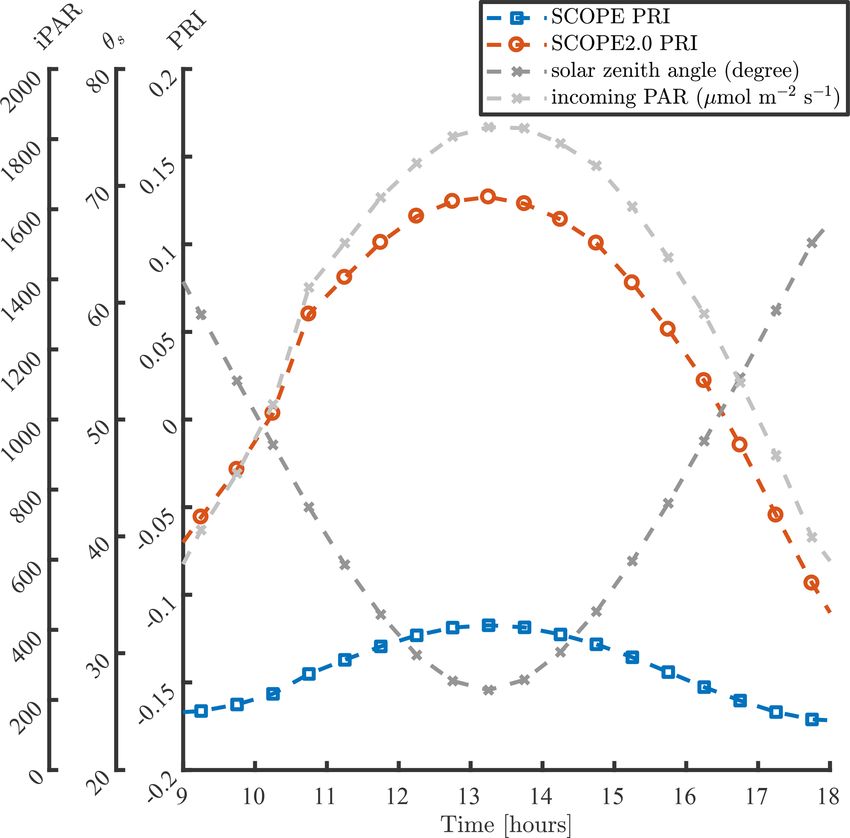
4698                                                                                                P. Yang et al.: SCOPE 2.0

surface–atmosphere exchange and identify changes therein.            SCOPE has been applied in a wide range of studies.
The most commonly used remote sensing indicator of vege-          Thanks to the coupling of photosynthesis and radiative trans-
tation biophysical and biochemical properties is reflectance      fer of fluorescence in the SCOPE model, it has been used
(Ollinger, 2011). For example, the MODIS (Moderate Res-           as a convenient tool for in-depth process-based studies to
olution Imaging Spectroradiometer) normalized vegetation          unravel the relationship between fluorescence and photosyn-
reflectance index (NDVI), and the Envisat MERIS Terres-           thesis (Damm et al., 2015; Verrelst et al., 2016; Migliavacca
trial Chlorophyll Index (MTCI) have been empirically corre-       et al., 2017). Besides, it has also been used for simulating
lated with canopy LAI and leaf chlorophyll content, respec-       directional anisotropy of satellite-measured surface tempera-
tively (Huete et al., 2002). For the past 10 years, remotely      tures (Duffour et al., 2015), for predicting evapotranspiration
sensed solar-induced chlorophyll fluorescence (SIF) has of-       (Galleguillos et al., 2011), and as a benchmark for other sim-
fered an additional way to monitor vegetation (Mohammed           pler radiative transfer models (Bian et al., 2020). Contem-
et al., 2019). SIF has been successfully used to estimate gross   porary simulations of satellite observations and plant physio-
primary production (GPP) (Guanter et al., 2014; Ryu et al.,       logical processes make SCOPE a useful tool to monitor vege-
2019) and stress detection (Ač et al., 2015; Rossini et al.,     tation dynamic response to environmental conditions (Zhang
2015). In addition to reflectance and SIF, thermal signals pro-   et al., 2014; Pacheco-Labrador et al., 2019).
vide insights in the physical processes of surface energy and        Since the original publication, SCOPE been extended with
water balance, such as demonstrated by the mapping of evap-       new features:
otranspiration globally with satellite thermal radiance (Ne-
                                                                      1. The Brightness–Shape–Moisture (BSM) soil re-
mani and Running, 1989; Allen et al., 2007).
                                                                         flectance model (Verhoef et al., 2018; Yang et al.,
   Combined radiative transfer and plant physiological mod-
                                                                         2020b) has been introduced.
elling is a promising way to investigate the exchange of en-
ergy, water, and carbon among soil, vegetation, and atmo-             2. The radiative transfer of fluorescence has been im-
sphere, and to develop remote sensing techniques for mon-                proved (Van der Tol et al., 2019).
itoring of vegetation functioning. Many factors affect the
signals observed from remote sensing, including the Sun–              3. Changes in reflectance due to dynamic xanthophyll pig-
observation geometry and the structure and composition of                ment changes have been included (Vilfan et al., 2018).
the Earth’s surface and atmosphere. A physically consis-              4. The RTMs in the SCOPE have been adapted for multi-
tent exploitation of remote sensing data therefore requires              layer canopies (Yang et al., 2017).
the modelling of radiative transfer in the soil–vegetation–
atmosphere system. Radiative transfer models (RTMs) de-              These new features have not been described together. In
scribe the relationship between vegetation characteristics and    the new version of SCOPE (SCOPE 2.0) presented here,
remote sensing observations obtained under varying Sun–           these improvements are coherently incorporated. Moreover,
observer geometry. However, for a complete understanding          the model has been optimized in many ways to improve the
of the role of vegetation in the energy budget of the Earth’s     computational efficiency and stability, and the options to pro-
surface, radiative transfer modelling is not sufficient. One      vide data input formats have been extended. We present a
also needs to model non-radiative processes of energy dis-        description of basic functionality of the model followed by
sipation via photosynthesis, phase transitions of water, heat     several recent developments.
storage, and turbulent heat exchange between the surface and
the atmosphere. This enables investigations beyond the mon-       2     General description of SCOPE
itoring of vegetation biophysical and biochemical properties,
towards monitoring of fluxes.                                     2.1    Starting points
   The Soil Canopy Observation of Photosynthesis and En-
ergy fluxes (SCOPE) model simulates the radiative transfer        SCOPE is designed to simulate photosynthetic, hydrological,
of incident light and thermal and fluorescence radiation emit-    and radiative transfer processes at the vegetated land surface.
ted by soil and plants, component temperatures, photosyn-         For these purposes, it combines several RTMs with a leaf
thesis, and turbulent heat exchange (van der Tol et al., 2009).   biochemical model and an aerodynamic resistance scheme.
In SCOPE, the radiative transfer and the non-radiative en-        These models provide simulations of emanating hyperspec-
ergy fluxes are computed in an assemblage of leaves and           tral radiance and net radiation Rn (via radiative transfer pro-
soil. The energy balance is maintained at all levels of spa-      cesses), photosynthesis rates (via photosynthetic processes),
tial aggregation. Maintaining an energy budget is necessary       and sensible heat flux H , latent heat flux λE, and ground heat
for the simulation of thermal radiation, which depends on the     flux G (via micrometeorological processes), for both individ-
within-canopy temperature distribution. To obtain this distri-    ual elements of the land surface (e.g. soil and leaves) and the
bution, stomatal aperture and latent and sensible heat fluxes     whole vegetation stand. In order to meet the requirements
of individual elements have to be resolved together with the      of broad applicability, the models are as physically based as
radiative fluxes in the vegetation canopy.                        possible.

Geosci. Model Dev., 14, 4697–4712, 2021                                            https://doi.org/10.5194/gmd-14-4697-2021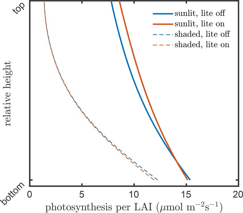
P. Yang et al.: SCOPE 2.0                                                                                                    4699

   The central idea of SCOPE is the modelling of interactions       tion is the (optional) modelling of the soil heat budget with a
between radiative and non-radiative fluxes among elements           thermal inertia approach, which is described in Sect. 3.4.
of the vegetation canopy. Remote sensing signals, such as re-          In the spectral domain, SCOPE simulates visible to ther-
flectance, fluorescence, and thermal radiance, are the output       mal infrared radiance from 0.4 to 50 µm as observed above
of these interactions. The modelling of radiative fluxes fa-        the canopy. The spectral resolutions in the spectral regions
cilitates the simulation of optical properties (i.e. reflectance,   from 0.4 to 2.5 µm, from 2.5 to 15 µm, and from 15 to 50 µm
transmittance, and absorptance) of soil, leaves, and canopies.      are 1, 100, and 1000 nm, respectively. It also covers the flu-
This is complemented with the modelling of non-radiative            orescence spectral region from 640 to 850 nm with a res-
fluxes in vegetation canopies, respecting energy conservation       olution of 1 nm. It is noted that the spectral resolutions in
at all levels of spatial aggregation from the photosystem to        these regions are easily adapted to simulation requirements
the whole stand. The energy budget is determined by both            and spectral input data.
the radiative transfer of incident and emitted (thermal) radi-
ation, and the exchange of (latent) heat with the atmosphere.       2.3     Structure of the model
The surface temperature is resolved as the outcome of this
balance.                                                            The model code at the highest hierarchical level, SCOPE,
                                                                    calls submodels which operate in series. The main submod-
                                                                    els are listed in Table 1. Besides the listed submodels for ra-
2.2   Model domain and representation
                                                                    diative transfer and energy balance, SCOPE requires func-
                                                                    tions for input, output, and some supporting functions (such
In the spatial domain, the typical representation of land sur-      as Planck’s equation). Therefore, all the functions used in
faces in SCOPE is a vegetation layer consisting of leaves           SCOPE can be organized into four types: (1) RTMs, (2) mod-
bounded underneath by a soil surface. The leaves in the             ules for energy balance, (3) input–output functions, and
canopy can have different orientations, which are character-        (4) supporting functions.
ized by 13 different leaf zeniths and 36 different leaf az-
imuths. The probability of the occurrence of each leaf orien-       2.3.1    RTMs
tation among 13 × 36 classes is quantified by using the leaf
inclination distribution function (LIDF). Thus, the model is        SCOPE includes seven RTMs, which together simulate the
more realistic than big-leaf and two-leaf models. Neverthe-         spectrally resolved radiance emanating from the vegetation:
less, the representation of the vegetation layer is one dimen-      one for the soil (BSM, only available in SCOPE 2.0, Ver-
sional in the sense that fluxes in the vertical (z) direction       hoef et al., 2018; Yang et al., 2020b), one for the leaf (Flus-
are considered only. This implies that even if the model is         pect, Vilfan et al., 2016, 2018), and five for the whole stand,
applied pixel by pixel in a spatial grid, the horizontal inter-     i.e. the combined system of soil and foliage. They include
actions are not considered. Thus, typical 3-D effects in the        one RTM for incident radiation from the Sun and the sky
vegetation, such as boundary effects at the edge of fields          (RTMo), two for thermal radiation emitted by the soil and
or forests, or effects of topography and horizontal heat ad-        vegetation (RTMt_sb and RTMt_planck), one for chlorophyll
vection are not included. Furthermore, radiative transfer is        fluorescence (RTMf, van der Tol et al., 2009; Van der Tol
based on turbid medium representations of the leaf and the          et al., 2019), and one for the dynamic modulations of leaf
whole canopy. This means that the clumping effect is not            reflectance and transmittance due to pigment changes in the
included in the current model. Except for radiation, within-        xanthophyll cycle (RTMz, only available in SCOPE v1.70 or
canopy variation of meteorological conditions (e.g. humidity        later, Vilfan et al., 2018).
and air temperature) is not fully simulated, and these meteo-          Four types of fluxes are involved in the radiative trans-
rological factors are differentiated only at three levels: above    fer processes, namely a direct solar flux, two hemispheri-
the roughness vegetation layer, in, and below the layer.            cal (semi-isotropic) diffuse fluxes (up- and downward), and
   In the temporal domain, SCOPE assumes steady-state con-          a flux in the direction of viewing. Following the Kubelka–
ditions. This means that a simulation with SCOPE outputs            Munk theory, the radiative transfer in the vertical direction
the energy and spectrally resolved radiation budgets of the         is expressed with a set of linear differential equations (Ver-
surface for a single set of surface and weather characteristics     hoef, 1984). These equations are solved either with analytical
at one moment in time. The lack of memory of state variables        or numerical approaches. This four-stream radiative transfer
in time also means that storage of carbon and water is not          theory is applied in SCOPE, and analytical solutions to the
considered, and similarly, vegetation growth is not simulated.      radiative transfer problems are essentially based on the ap-
A complete run of SCOPE may consist of many simulations,            proach given in Verhoef (1984) and Verhoef (1985). SCOPE
either for one location as a function of time, or for differ-       2.0 employs an updated unified four-stream radiative transfer
ent locations or surface types, but the simulations in such a       theory for multi-layer vegetation canopies and uses differ-
sequence are treated independently without interactions, and        ent solutions for the radiative transfer problems. A complete
thus the order of model simulations is arbitrary. One excep-        derivation of the solutions is given in Yang et al. (2020c).

https://doi.org/10.5194/gmd-14-4697-2021                                              Geosci. Model Dev., 14, 4697–4712, 2021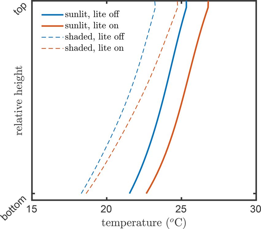
4700                                                                                                        P. Yang et al.: SCOPE 2.0

Table 1. Main submodels in SCOPE.

    Submodels                 Main functions       Main input                                 Main output
    BSM                       simulating soil      soil moisture, brightness, and two         anisotropic soil reflectance
                              reflectance          spectral-shape-related parameters
    Fluspect                  leaf RTM             leaf biophysical properties                leaf reflectance, transmittance, and
                                                                                              fluorescence emission matrices
    RTMo                      RTM for incident     canopy structure, leaf reflectance,        canopy reflectance, radiation absorbed
                              radiation            transmittance, and soil reflectance        by individual leaves
    RTMf                      RTM for fluores-     canopy structure, leaf reflectance,        fluorescence of individual leaves and of
                              cence fluxes         transmittance, soil reflectance, and       the whole canopy
                                                   fluorescence emission matrices
    RTMt_sb/RTMt_planck       RTM for thermal      leaf temperature, incoming thermal         thermal emission of individual leaves
                              fluxes               radiation, emissivity of soil and leaves   and of the whole canopy
    RTMz                      RTM for fluxes       leaf-absorbed radiation, canopy struc-     dynamic modulations of canopy
                              induced by the       ture, leaf reflectance, transmittance,     reflectance
                              xanthophyll cycle    soil reflectance
    biochemical               biochemical          leaf-absorbed radiation, leaf tempera-     photosynthesis rate, fluorescence emis-
                              model for            ture, photosynthetic parameters            sion efficiency and heat dissipation
                              photosystem
                              energy
                              partitioning
    ebal                      energy balance       leaf-absorbed radiation, leaf tempera-     sensible and latent heat fluxes
                              module               ture

2.3.2   Energy balance module                                         stomatal model (Van der Tol et al., 2014), while for the soil, a
                                                                      surface resistance applies which is either a pre-defined input
The energy balance module in SCOPE minimizes the energy               or an empirical function of soil moisture.
balance closure error eebal ,

eebal = Rn − H − λE − G,                                     (1)      2.3.3      Leaf biochemical model

for all leaf and soil elements by iteratively updating their          The biochemical model simulates the energy partitioning
temperature. In this equation, Rn is the net radiation, H the         into fluorescence, heat, or photochemistry in photosystems
sensible heat flux, λE the latent heat flux, and G the ground         (Maxwell and Johnson, 2000; Van der Tol et al., 2014). It
heat flux (zero for leaf elements), all in W m−2 . In the energy      is based on a conventional photosynthesis model of Collatz
balance, chemical conversions (photosynthesis and respira-            et al. (1991) for C3 and Collatz et al. (1992) for C4 vegeta-
tion) and fluorescence are neglected.                                 tion, in which photosynthetic rates (or photosynthetic light-
   The net radiation is obtained after spectral integration of        use efficiency) are simulated as a function of leaf tempera-
the radiative transfer modules for incident radiation (RTMo)          ture, ambient radiation levels, intercellular CO2 concentra-
and internally generated thermal radiation (RTMt). The ra-            tions Ci , and other leaf physiological parameters (e.g. pho-
diative transfer for incident radiation is computed before the        tosynthetic pathways, maximum carboxylation rate Vcmo ). A
energy balance closure loop, while the internally generated           difference with some other canopy-scale models (e.g. BEPS)
thermal radiation is calculated within this loop because of its       is that SCOPE applies the photosynthesis models at leaf level
dependence on leaf and soil temperatures. The sensible and            (disaggregated), whereas many other models apply these
latent heat fluxes are calculated with an aerodynamic resis-          models at aggregated (big-leaf or Sun-shade two-leaf mod-
tance scheme, where resistances for the leaf and soil bound-          els) scales.
ary layer, the vegetation layer, and the atmospheric surface             Van der Tol et al. (2014) established empirical relation-
layer apply. The aerodynamic resistances depend on atmo-              ships between fluorescence emission efficiency and photo-
spheric stability, wind speed, and surface roughness (van der         synthetic light-use efficiency under various environmental
Tol et al., 2009). For latent heat flux of leaves, a stomatal         conditions by using active fluorescence measurements. With
resistance is calculated with a combined photosynthesis and           these relationships, the fraction of the absorbed radiation by

Geosci. Model Dev., 14, 4697–4712, 2021                                                   https://doi.org/10.5194/gmd-14-4697-2021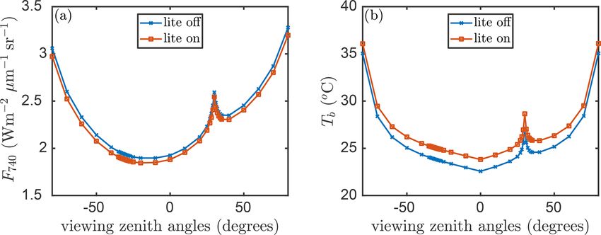
P. Yang et al.: SCOPE 2.0                                                                                                  4701

a leaf emitted as fluorescence and dissipated as heat can be      2.4     Model inputs and outputs
simulated.
                                                                  2.4.1    Input variables for soil, vegetation, and
2.3.4   Interactions among the submodels                                   meteorology
Figure 1 is a schematic overview of the SCOPE model struc-
ture, which also shows the connections among the submod-          The inputs of the SCOPE model comprise soil, leaf, and
els. A full list of input parameters is provided in Table 2.      canopy properties as well as Sun–observer geometry and me-
A simulation with SCOPE starts with calculating soil re-          teorological conditions. Besides the intermediate variables,
flectance (BSM), the leaf reflectance, and transmittance and      which are passed between the submodels, the main input
fluorescence emission excitation matrices (Fluspect). These       variables of SCOPE are given in Table 2.
simulations of soil and leaf optical properties, together with       Leaf biophysical and biochemical parameters characterize
canopy structure and irradiance, are the input of canopy          leaf pigment, water, and dry matter contents, which deter-
RTMs. The submodel for radiative transfer of solar and sky        mine leaf optical properties. Canopy structural parameters
radiation (RTMo) takes leaf optical properties and soil re-       describe the arrangement of the leaves in the canopy. Sun–
flectance as input and outputs canopy reflectance and radia-      observer geometry is determined by the Sun and observer’s
tion fluxes including the net absorbed solar radiation by soil    zenith angles and their absolute azimuth difference. Both
and leaves. RTMf takes the leaf fluorescence emission exci-       the canopy structural parameters and Sun–observer geome-
tation matrices and the radiation fluxes as input and simulates   try strongly affect remote sensing signals observed above the
canopy fluorescence.                                              canopy.
   The radiative transfer of emitted thermal radiation relies        The meteorological inputs for SCOPE include the typi-
on the temperatures of soil and leaves, which are not known       cal synoptic weather variables of air temperature, humidity,
a priori. For this reason, the thermal radiative transfer model   wind speed, and air pressure, and the concentrations of oxy-
is carried out in the energy balance closure loop as described    gen and carbon dioxide. All these inputs are required close to
in Sect. 2.3.2. For the purpose of computational efficiency,      the Earth’s surface. The height above the surface of the ter-
the radiative transfer of emitted thermal radiation is carried    rain for which they are specified must be given in the input,
out in broadband in this loop by using RTMt_sb. The letters       as input z, typically 2.5 times the vegetation height. Thus, z
“sb” denote the use of the Stefan–Boltzmann law to describe       is not the height of the terrain above sea level but rather the
the spectrally integrated radiance from a leaf or soil in terms   height above the terrain at in surface layer, where the wind
of its temperature. Leaf temperature is also used together        profile is logarithmic. The value of z must be given in the
with the radiation absorbed by leaf chlorophyll pigments and      input as it is used to calculate the aerodynamic roughness of
other leaf physiological parameters to simulate photosystem       the surface.
energy partitioning in the biochemical model (Van der Tol
et al., 2014). The energy balance residual is used to update      2.4.2    Input irradiance for the atmosphere boundary
the initial estimate of temperature of each element.                       condition
   After energy balance closure, the thermal radiation fluxes
are simulated as spectrally resolved in the observation direc-    In addition to the variables listed in Table 2, SCOPE requires
tion by using RTMt_planck, where “planck” denotes the use         the radiative properties of the atmosphere as an upper bound-
of Planck’s law to describe the spectrally resolved radiance      ary condition. They can be provided in two different ways.
from a leaf or soil in terms of its temperature. The radiative       The first option is to provide irradiance at the bottom of
transfer of the emitted fluorescence is simulated with RTMf.      the atmosphere (BOA) in the form of a file with two columns
This module uses the radiative fluxes interacting with leaves     representing the spectra of direct solar irradiance Esun and
as simulated with RTMo, and the fluorescence emission ma-         diffuse sky irradiance Esky [W m−2 µm−1 sr−1 ], respectively.
trices simulated with Fluspect, to simulate leaves’ fluores-      These spectra could either be measured in the field or gener-
cence emission, which is aggregated to canopy fluorescence        ated with an atmospheric RTM (e.g. MODTRAN, Berk et al.,
signals. Finally, the effect of (small) changes in reflectance    1999). Using an atmospheric RTM has the disadvantage that
and transmittance due to the illumination and temperature-        Esky may not be accurate, because Esky depends also on the
dependent xanthophyll epoxidation state are simulated with        surface (canopy) reflectance in the surroundings, which may
RTMz.                                                             not be known a priori in the atmospheric radiative transfer
                                                                  simulation. Therefore, if the surface reflectance assumed in
                                                                  the atmospheric radiative transfer simulation largely differs
                                                                  from the canopy reflectance produced by SCOPE, errors in
                                                                  Esky occur.
                                                                     The second and preferred option is using an atmospheric
                                                                  RTM to generate some optical properties of the atmosphere

https://doi.org/10.5194/gmd-14-4697-2021                                            Geosci. Model Dev., 14, 4697–4712, 2021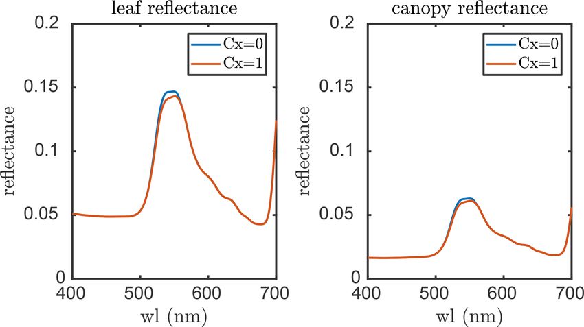
4702                                                                                                         P. Yang et al.: SCOPE 2.0

Figure 1. Schematic overview of the SCOPE model structure. For a complete list of input data, see Table 2.

rather than the direct output of Esky and Esun . The optical
properties should include the following coefficients:                  Esun = Es cos(θs )τss
  – Es cos(θs ), the product of the solar irradiance at the top        Esky =
    of the atmosphere (TOA) and the cosine of the solar                 Es cos(θs )(τsd + τss ρdd rsd ) + π((1 − rdd )Ls ρdd + La )
    zenith angle; this product is the irradiance at TOA pro-                                                                        , (2)
                                                                                                1 − ρdd rdd
    jected on the surface (W m−2 µm−1 sr−1 );
                                                                       where rsd and rdd are the surface reflectance for direct and
  – ρdd , the diffuse reflectance of the atmosphere (i.e. the          diffuse incoming radiation, respectively, and Ls the thermal
    spherical albedo);                                                 emission by the (vegetated) surface (W m−2 µm−1 sr−1 ). All
                                                                       of them are simulated with SCOPE. The overbars denote
  – τss , the direct atmospheric transmittance in the direction        the spectral averaging to the SCOPE resolution (1 nm in the
    of the Sun;                                                        visible–near infrared, VNIR). Note that τss and ρdd are ag-
  – τsd , the diffuse atmospheric transmittance for solar inci-        gregated to the SCOPE resolution separately, but also the
    dence; and                                                         product τss ρdd , in order to accommodate spectral correlation
                                                                       effects in the finite bands. The coupling with the atmosphere
  – La , the thermal emission by atmosphere at BOA to-                 is described in detail in Verhoef et al. (2018) and Yang et al.
    wards the surface (W m−2 µm−1 sr−1 ).                              (2020b).
                                                                          Finally, SCOPE offers the possibility to provide additional
   The coefficients listed can be extracted from MODTRAN               values for the spectrally integrated irradiance (direct solar ra-
simulations by using the T18 system, which is described in             diation Esun plus Esky ) over the ranges from 0.4 to 2.5 µm
detail in Verhoef et al. (2018). A database of the optical co-         and 2.5 to 50 µm. These are the input fields Rsi and Rli ,
efficients for several typical atmospheric conditions is pro-          respectively. However, it is not necessary to specify these
vided together with the SCOPE model. With these coeffi-                inputs, because the broadband irradiances Rsi and Rli are
cients, SCOPE can simulate the BOA direct and diffuse ir-              already calculated internally as the integral of the irradi-
radiance spectra in the module RTMo with consideration of              ance spectra. If the values for these two inputs are speci-
surface–atmosphere interactions. The BOA irradiances Esun              fied, then the solar and sky irradiance spectra Esun plus Esky
and Esky are calculated in the function RTMo as                        are linearly scaled (each by the same factor so that the ra-
                                                                       tio Esun /Esky remains unaltered) in the two spectral regions
                                                                       separately to match the values provided for Rsi and Rli . This
                                                                       option can be useful if time series of synoptic weather data

Geosci. Model Dev., 14, 4697–4712, 2021                                                  https://doi.org/10.5194/gmd-14-4697-2021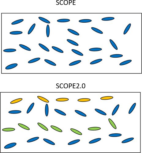
P. Yang et al.: SCOPE 2.0                                                                                                            4703

Table 2. Main input variables of SCOPE.

        Symbol   Abbreviation     Unit           Submodel                Description
        Cab      Cab              [µg cm−2 ]     Fluspect                leaf chlorophyll concentration
        Cca      Cca              [µg cm−2 ]     Fluspect                leaf carotenoid concentration
        Cw       Cw               [cm]           Fluspect                equivalent water thickness in leaves
        Cs       Cs               []             Fluspect                leaf senescence parameters
        Cdm      Cdm              [g cm−2 ]      Fluspect                leaf dry matter content
        Cant     Cant             [µg cm−2 ]     Fluspect                anthocyanin content
        N        N                []             Fluspect                leaf structure parameter
        ρt       rho_thermal      []             Fluspect                broadband leaf thermal reflectance
        τt       tau_thermal      []             Fluspect                broadband leaf thermal reflectance
        L        LAI              []             canopy RTMs             one-sided projected leaf area per unit ground area
        hc       hc               [m]            canopy RTMs             vegetation height
        LIDFa    LIDFa            []             canopy RTMs             leaf inclination parameter for the mean leaf zenith angle
        LIDFb    LIDFb            []             canopy RTMs             bimodality of the leaf angle distribution
        θs       tts              [degree]       canopy RTMs             solar zenith angle
        θo       tto              [degree]       canopy RTMs             viewing zenith angle
        ψ        psi              [degree]       canopy RTMs             absolute azimuth difference between solar and viewing
        Rsi      Rin              [W m−2 ]       canopy RTMs             shortwave irradiance
        Rli      Rli              [W m−2 ]       canopy RTMs             longwave irradiance
        pa       p                [hPa]          energy balance          air pressure
        Ta       T                [◦ C]          energy balance          air temperature
        u        u                [m s−1 ]       energy balance          wind speed
        ea       ea               [hPa]          energy balance          vapour pressure
        VPD      VPD              [hPa]          energy balance          vapour pressure deficit
        RH       RH               [fraction]     energy balance          relative humidity
        z        z                [m]            energy balance          measurement height
        rst      rs_thermal       []             energy balance          broadband soil thermal reflectance
        2        SMC              []             BSM, energy balance     volumetric soil moisture content at the surface
        B        BSMBrightness    []             BSM                     soil brightness
        ϕ        BSMlat           [degree]       BSM                     soil “latitude” parameter (not geographical)
        λ        BSMlon           [degree]       BSM                     soil “longitude” parameter (not geographical)
        Ca       Ca               [ppm]          biochemical model       atmospheric CO2 concentration
        Vcmo     Vcmo             [µmol m−2 ]    biochemical model       carboxylation capacity at 25 ◦ C
        m        m                []             biochemical model       Ball–Berry stomatal parameter (slope)
        B0       Ball–Berry0      []             biochemical model       Ball–Berry stomatal parameter (intercept)

are used as input, and if it is computationally not feasible to    sorbed PAR by chlorophyll. Most of the stored outputs of
carry out atmospheric radiative transfer simulations for every     SCOPE are for the whole canopy, although similar variables
time step separately. For coupled surface–atmosphere simu-         of leaves are also computed internally in SCOPE. Some in-
lations, this is not recommended, because of obvious incon-        termediate variables, e.g. leaf-absorbed PAR by chlorophyll
sistencies between SCOPE and the atmospheric model. In             and fluorescence spectra, are simulated but not stored as the
that case, the input fields for Rsi and Rli must be left blank.    final outputs.

2.4.3    Model outputs
                                                                   3     Major improvements of SCOPE 2.0 compared with
In Table 3, the main outputs of SCOPE are listed. The gen-               SCOPE
eral output of SCOPE includes (1) spectral simulations of
radiance in the viewing direction and upward flux for the          3.1    Implementation of the BSM soil reflectance model
whole upper hemisphere from optical to thermal domain in-
cluding fluorescence; (2) radiation budget, such as incoming       In the first published version of SCOPE, the soil reflectance
and outgoing radiation for shortwave from 0.5 to 2.5 µm and        spectrum was an input variable. The users should either pro-
longwave from 2.5 to 50 µm; (3) fluxes such as sensible heat,      vide a measured soil spectrum or select one from the soil
latent heat, and the ground heat flux for canopy, soil, and        reflectance library incorporated in the SCOPE model. In
the combined system; and (4) canopy absorption, such as ab-        SCOPE 2.0, we provide the users the option to simulate soil

https://doi.org/10.5194/gmd-14-4697-2021                                                Geosci. Model Dev., 14, 4697–4712, 2021
4704 P. Yang et al.: SCOPE 2.0
Table 3. SCOPE outputs.
Output Description Unit
Spectral simulation
Eout_spectrum Hemispherical leaving irradiance [W m−2 µm−1 ]
Lo_spectrum Radiance in the viewing direction [W m−2 µm−1 sr−1 ]
fluorescence Fluorescence radiance in the viewing direction [W m−2 µm−1 sr−1 ]
fluorescence_hemis Hemispheric leaving fluorescence irradiance [W m−2 µm−1 ]
reflectance TOC reflectance in the viewing direction []
Vegetation
aPAR PAR absorbed by the vegetation [µmol m−2 s−1 ]
aPARbyCab PAR absorbed by chlorophyll [µmol m−2 s−1 ]
aPARbyCab_en PAR energy absorbed by chlorophyll [W m−2 ]
Photosynthesis Canopy photosynthesis rate [µmol m−2 s−1 ]
LST Black-body radiometric land surface temperature [K]
Fluxes
Rnctot Net radiation of canopy [W m−2 ]
lEctot Latent heat flux of canopy [W m−2 ]
Hctot Sensible heat flux of canopy [W m−2 ]
Actot Net photosynthesis of canopy [W m−2 ]
Tcave Average canopy temperature [◦ C]
Rnstot Net radiation of soil [W m−2 ]
lEstot Latent heat flux of soil [W m−2 ]
Hstot Sensible heat flux of soil [W m−2 ]
Gtot Soil heat flux [W m−2 ]
Tsave Average soil temperature [◦ C]
Rntot Total net radiation [W m−2 ]
lEtot Total latent heat flux [W m−2 ]
Htot Total sensible heat flux [W m−2 ]
Radiation
ShortIn Incoming shortwave radiation [W m−2 ]
LongIn Incoming longwave radiation [W m−2 ]
HemisOutShort Hemispherical outgoing shortwave radiation [W m−2 ]
HemisOutLong Hemispherical outgoing longwave radiation [W m−2 ]
Lo Radiance in observation direction [W m−2 sr−1 ]
Lot Thermal radiance in observation direction [W m−2 sr−1 ]
Lote Emitted radiance in observation direction [W m−2 sr−1 ]
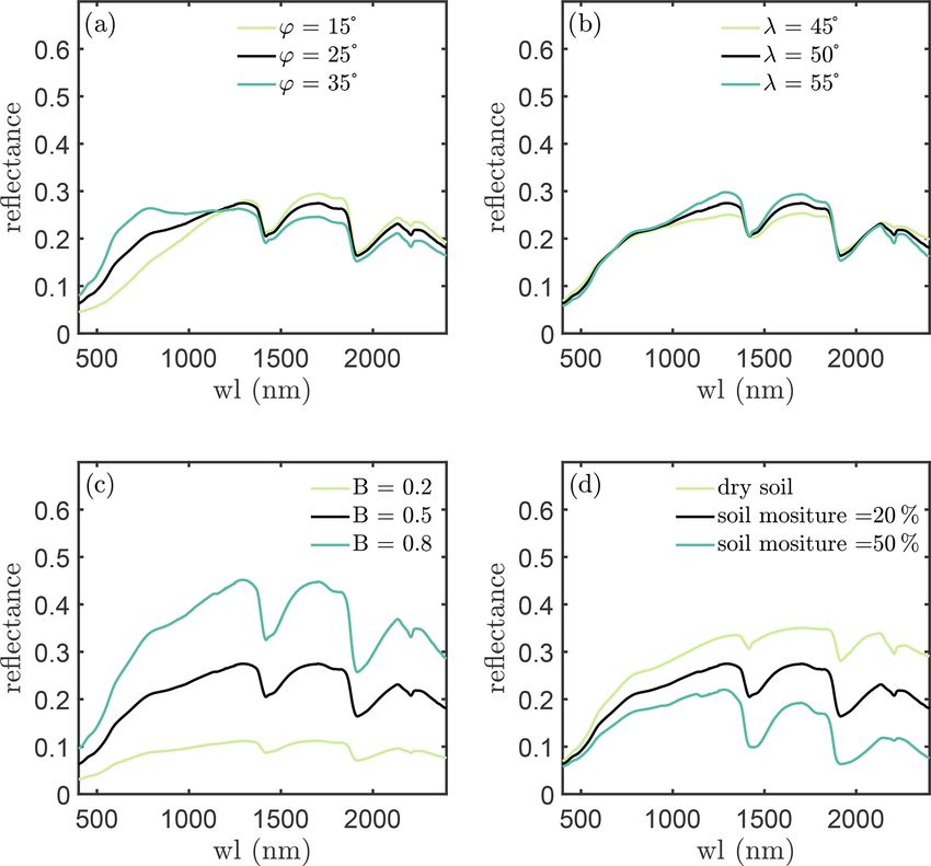
reflectance thanks to the implementation of a soil reflectance “intensity” of soil reflectance and the “shape” of soil re-
model. flectance is controlled by ϕ and λ. Soil moisture affects re-
The BSM model simulates the isotropic soil reflectance. flectance intensity over all wavelengths but reflectance at the
This model is based on an empirical reflectance model of water absorption bands is more sensitive to soil moisture.
dry soil (Verhoef et al., 2018; Jiang and Fang, 2019) and Soil moisture effects on reflectance are considerably simi-
incorporates the effects of soil moisture by using the water lar to the effects of soil brightness, and soil is dark when it is
film coating approach (Ångström, 1925; Yang et al., 2020b). wet as explained in Lekner and Dorf (1988).
To simulate reflectance of dry soil, the model requires soil
brightness (B) and two spectral-shape-related parameters (ϕ 3.2 Inclusion of dynamic reflectance induced by the
and λ) as inputs. Soil moisture is necessary for simulating xanthophyll cycle
wet soil reflectance.
Figure 2 shows the effects of the four parameters on soil A new feature in SCOPE 2.0 is modelling the photochemi-
reflectance. It is evident that soil brightness only affects the cal reflectance dynamics induced by the xanthophyll cycle at
Geosci. Model Dev., 14, 4697–4712, 2021 https://doi.org/10.5194/gmd-14-4697-2021P. Yang et al.: SCOPE 2.0 4705
Figure 3. The effects of the xanthophyll cycle on leaf and canopy
reflectance simulated with SCOPE 2.0. Cx is a factor for the de-
epoxidation state (DEPS) of xanthophyll cycle pigments.
ilar to RTMf in the sense that both the xanthophyll cycle
and fluorescence emission lead to small changes in (appar-
ent) reflectance but for different spectral regions (i.e. 500–
Figure 2. Reflectance simulations with the BSM model. The black 570 and 640–850 nm, respectively). RTMf and RTMz take
curves in each panel are the same simulation. fluorescence emission efficiency and Cx (simulated from the
leaf biochemical model), respectively, as inputs, of which the
magnitudes vary among individual leaves due to their ambi-
both leaf and canopy levels. In the original leaf RTM Flus- ent light intensities, temperature, etc. Figure 3 depicts an ex-
pect (Vilfan et al., 2016), leaf optical properties are deter- ample of the effects of Cx on the leaf and canopy reflectance
mined by leaf biophysical properties. However, in natural as simulated by SCOPE 2.0 with the default model inputs.
conditions, the xanthophyll cycle that is involved in photo- Although the effects on canopy reflectance seem small, they
protection mechanisms under excess light can provoke a could be helpful for monitoring the variation in DEPS.
change in reflectance and transmittance as the composition of Figure 4 compares simulations of PRI in a day with
the pigment pool is regulated. Changes in the de-epoxidation SCOPE and SCOPE 2.0. In these simulations, the default
state (DEPS) of xanthophyll cycle pigments (e.g. violax- model inputs are used except for the incoming radiation and
anthin and zeaxanthin) can be observed as changes in the solar zenith angles. The values of incoming radiation and so-
leaf absorption of light with wavelengths between 500 and lar zenith angles (θs ) are assigned according field measure-
570 nm. These spectral changes can be a good remote sensing ments presented in Yang et al. (2020a) (i.e. on day 232 of the
indicator of the photosynthetic efficiency. The photochemical dataset in the referred paper). The comparison demonstrates
reflectance index (PRI, R 570 −R531
R570 +R531 ) proposed by Gamon et al.
that the inclusion of dynamic reflectance induced by the xan-
(1992) is a example of a measure for the effects of xantho- thophyll cycle has a clear impact on the simulation of diur-
phyll cycle pigments on the reflectance. It takes changes in nal changes in PRI. In SCOPE, diurnal variation of PRI is
reflectance at 531 nm to estimate DEPS with reflectance at mainly regulated by Sun–observer geometry, since leaf bio-
570 nm as a reference to correct changes in reflectance in- physical properties and canopy structure are kept unchanged
duced by other factors, such as Sun–observer geometry. in a day. Because the bidirectional reflectance distribution
Vilfan et al. (2018) incorporated the effects of the xantho- function (BRDF) effects on reflectance at 531 and 570 nm
phyll cycle on leaf optical properties in Fluspect and devel- are similar, they cancel out in PRI, and the diurnal varia-
oped the Fluspect-CX model. The main idea of Fluspect-CX tion of PRI simulated with SCOPE is small. Compared with
is to use in vivo specific absorption coefficients for two ex- SCOPE, SCOPE 2.0 considers the changes in leaf pigment
treme states of carotenoids, representing the two extremes pool induced by the xanthophyll cycle in response to the vari-
of the xanthophyll de-epoxidation. A “photochemical re- ation of incoming radiation besides the BRDF effects. The
flectance parameter” (Cx) is employed to describe the in- excessive incoming radiation during midday leads to larger
termediate states as a linear mixture of these two states. Cx Cx values than in the morning and afternoon, and higher af-
controls the specific absorption coefficient of carotenoids in ternoon than morning temperatures to higher afternoon Cx,
a leaf and thus affects leaf reflectance and transmittance. and thus more significant diurnal variation of PRI.
The propagation of changes in leaf reflectance and trans-
mittance induced by the xanthophyll cycle to TOC re-
flectance is carried out with RTMz, which is largely sim-
https://doi.org/10.5194/gmd-14-4697-2021 Geosci. Model Dev., 14, 4697–4712, 20214706 P. Yang et al.: SCOPE 2.0
Figure 5. Representations of canopies in SCOPE and in SCOPE
2.0.
Figure 4. The effects of the xanthophyll cycle on simulation of PRI
RTMs in SCOPE 2.0 remain structurally the same with the
in a day.
original SCOPE. However, a more general solution of the ra-
diative transfer problems is used. Compared to the classic
SAIL analytical solution, SCOPE 2.0 (and mSCOPE) em-
3.3 Adaption of the RTMs for multi-layer canopies ploys the adding method to solve the radiative transfer prob-
lems. The application of the adding method for TOC re-
The original SCOPE model assumes that vegetation canopies flectance simulation is given in Verhoef (1985). Yang et al.
are vertically homogeneous and horizontally infinite, as its (2017) extended this method to calculating the radiative flux
radiative transfer routines are based on the classical 1-D profiles in the canopy. The procedure is summarized as fol-
SAIL model (Verhoef, 1984). The vertical heterogeneity lows: (1) divide the vertical layer into n thin homogeneous
of leaf biophysical and biochemical properties may have a layers; (2) start from the bottom homogeneous layer, calcu-
large effect on the bi-directional reflectance, fluorescence, late the surface reflectance of the combined system of the
and photosynthesis of vegetation canopies. To allow simula- bottom surface (e.g. soil) and this layer; (3) add a new homo-
tions of vertical heterogeneous canopies, Yang et al. (2017) geneous vegetation layer above the surface of the previous
modified the RTMs in SCOPE and developed a new branch system in step 2, and calculate the surface reflectance of the
of SCOPE, called mSCOPE. SCOPE 2.0 incorporates the new system; (4) repeat step 3 until all homogeneous layers
essence of mSCOPE on radiative transfer modelling and are added. (5) Once the surface reflectance at each vertical
adapts the capability to simulate reflectance, fluorescence level is obtained, the fluxes profile can be computed from top
and photosynthesis of vertically heterogeneous canopies (as to bottom, given the incident fluxes at top of the canopy. For
illustrated in Fig. 5). In comparison with the original SCOPE, the radiative transfer of fluorescence and thermal radiation,
SCOPE 2.0 accepts vertical profiles of leaf properties (such the emission from leaves and soil should be included as ex-
as chlorophyll content) as inputs. This is done via a table tra radiation sources besides the incident fluxes at the top of
in which optical properties can be specified for user-defined the canopy. In SCOPE 2.0, the value of n is set as 10 times
LAI intervals. If single values of the Fluspect parameters the LAI rather than a fixed value of 60 in mSCOPE, because
in Table 2 are provided, the model will assume the canopy this ensures the LAI of one elementary layer is small enough
is vertically homogeneous. The true heterogeneity of leaves (i.e. LAI of a thin layer, iLAI < 0.1), and the use of less el-
within a vegetation canopy may be too large to fully imple- ementary layers improves the computational efficiencies of
ment in the model. Thus, a simplification of the canopy may the RTMs.
be needed: two- or three-layer representations are most com-
mon. For example, forests usually have understorey and over- 3.4 An alternative way to estimate the ground heat flux
storey, and crops at the senescent stage have two or three dis-
tinct layers with brown or green leaves. However, it is noted In SCOPE, the ground heat flux is calculated for the sunlit
that more layers are possible in SCOPE 2.0 for specific pur- and shaded soil (the heat storage changes in the canopy are
poses as shown in Yang et al. (2017). not considered). In the original SCOPE model, this was ei-
Geosci. Model Dev., 14, 4697–4712, 2021 https://doi.org/10.5194/gmd-14-4697-2021P. Yang et al.: SCOPE 2.0 4707
ther a constant fraction of 0.35 of the net radiation on the soil where δebal /δT is the first derivative of the energy balance
or calculated with the force restore method of Bhumralkar closure error to temperature, and W is a weighting for the
(1975). SCOPE 2.0 offers an alternative way to estimate the step size. The derivative is estimated analytically:
ground heat flux as a function of the soil temperature time se-
δebal /δT = ρ · cp /ra + ρ · λ · MH2 O /Mair /p · s/(ra + rs )
ries with the method of Wang and Bras (1999). The ground
heat flux is determined by the gradient of soil temperature + 4εσ (Told + 273.15)3 (7)
in the profile underneath the soil surface. The subsurface is Equation (6) is a linearization of the relation between tem-
outside the model domain of SCOPE, and therefore the soil perature and energy balance error. This linearization is esti-
temperature gradient is not simulated. However, this vertical mated analytically, which is much faster than calculating the
gradient may equivalently be expressed the by the half-order derivative numerically. In the estimate, it is assumed that the
time derivative of the surface temperature (Wang and Bras, incident irradiance on the leaves (or soil) does not change.
1999). This enables the estimation of G from the time his- This is an approximation. The internally (in the canopy) gen-
tory of the surface temperature: erated incident irradiance depends on the temperature of the
Zt neighbouring leaves, which is updated in the next iteration
√ T (s) step as well. Further, it is assumed that the resistances ra and
G(t) = 0/ π ds, (3)
t −s rs do not change between iteration steps. This is an approxi-
t0
mation as well, as both depend on leaf and soil temperature.
where T is the soil temperature at time s, 0 Although these interactions cannot be resolved analytically,
[J m−2 s−1/2 K−1 ] is the thermal inertia of the soil, cal- Eq. (6) is a sufficiently accurate approximation of the first
culated from physical properties of the soil: derivative to obtain rapid energy balance convergence. Iter-
p ations continue until the maximum absolute closure error of
0 = cs · ρs · λs , (4) all leaf and soil elements is less than 1 W m−2 , and this is
usually achieved in less than 10 iteration steps. If energy bal-
where cs is the volumetric heat capacity of the soil ance closure is not achieved after 10 steps, then the weight-
[J kg−1 K−1 ], ρs the soil bulk density [kg m−3 ], and λs ing coefficient W is gradually decreased from 1 (i.e. smaller
[J m−1 s−1 K−1 ] the heat conductivity of the soil. In SCOPE update steps) to avoid the updated temperatures bouncing
2.0, a solution derived for a discrete time series of tempera- around the solution.
tures by Bennett et al. (2008) (Eq. A3 therein) was adopted: In earlier versions of SCOPE, a similar equation to Eq. (6)
12 has been used to update temperature in the energy balance
√ X Ti+1 − Ti √ p
G(t) = 20/ π ( t − si − t − si+1 ). (5) loop. However, the partial derivative of latent heat flux to
s − si
i=1 i+1 temperature was not included in the equation. The improve-
ment in SCOPE 2.0 has substantially reduced the number of
This approach is only meaningful if consecutive simula- required iterations due to a more complete estimate of the
tions are carried out in a time series, in which the diurnal derivative.
variation of temperature is reproduced (at least one simula-
tion per 3 h time step). The approximation of G = 0.35Rns 3.6 Angular aggregation of sunlit leaves
should be used for cases in which the state of the soil heat
reservoir cannot be known, for example, if simulations are In the energy balance routine, the number of sunlit leaf ele-
carried out for pixels in a satellite image taken at a single ments that are considered is 13 leaf zenith × 36 leaf azimuth
moment in time. times 10 × LAI layers, while the number of shaded leaf el-
ements is 10 × LAI. Solving the energy budget for all these
3.5 Improvements in energy balance closure elements separately means that a closure of energy balance
should be achieved for each element and this is computation-
The energy balance loop starts by simulating the radiative ally demanding. SCOPE 2.0 offers the possibility to simulate
transfer of internally generated radiation with initial esti- the non-radiative energy fluxes, photosynthesis and gas ex-
mates of component temperatures, followed by the calcula- change for all inclination and azimuth angles of the sunlit
tion of aerodynamic and stomatal resistances (and photosyn- leaves combined (the ’lite’ option). This involves an aggre-
thesis), and the fluxes H , λE, and G. Finally, new estimates gation (weighted averaging) of net radiation over all leaf an-
of the component temperatures are calculated from the value gles, before entering the energy balance loop. One effective
of the energy balance closure error (1E) per leaf and soil leaf for the 13 × 36 sunlit leaf classes is used for each layer.
element. Newton’s method is used to estimate the new tem- The resulting number of elements is 10 × LAI for the sunlit
peratures, which are the starting point for the next iteration leaves and 10 × LAI for the shaded leaves. This significantly
in the loop. reduces the computation time of the energy balance routine.
ebal The consequence of this internal aggregation is that the all
Tnew = Told + W · , (6) sunlit leaves in a layer will have an identical temperature,
δebal /δT
https://doi.org/10.5194/gmd-14-4697-2021 Geosci. Model Dev., 14, 4697–4712, 20214708 P. Yang et al.: SCOPE 2.0
Figure 6. Layer-average kinetic temperatures of the leaves in the Figure 7. Layer photosynthesis per LAI in the vegetation canopy
vegetation canopy simulated by SCOPE 2.0 with the “lite” repre- simulated by SCOPE 2.0 with the “lite” representation on (red)
sentation on (red) and off (blue) of the vegetation, for sunlit (solid and off (blue) of the vegetation, for sunlit (solid lines) and shaded
lines) and shaded (dashed lines) leaves. (dashed lines) leaves.
gas exchange, photosynthesis rate, chlorophyll fluorescence
emission efficiency, and latent and sensible heat fluxes, inde-
pendent of their inclination towards the Sun. Figures 6 and 7
present examples for the effects of the angular aggregation on
the profiles of leaf temperature and photosynthesis simula-
tions, respectively. In these simulations, the default model in-
puts are used. Due to the simplifications in the energy balance
and biochemical part in the lite mode, the layer-average tem-
Figure 8. (a) Top-of-canopy fluorescence at 740 nm (F740 ) and
peratures become slightly higher for both sunlit and shaded (b) surface brightness temperature (Tb ) simulated by SCOPE 2.0
leaves (Fig. 6). A slight difference in photosynthetic produc- with the “lite” representation on (red) and off (blue) of the vegeta-
tion between the lite-on and lite-off modes can be found for tion versus viewing angles in the principle plane.
sunlit leaves, but the difference for shaded leaves is negli-
gible (Fig. 6). The photosynthetic production simulation for
the whole canopy changes by about 0.7 µmol m−2 s−1 (4 %) around 0.1 W m−2 µm−1 sr−1 and around 1◦ in the surface
when the lite mode is activated. The differences in leaf tem- temperature simulation. The difference in radiance is mini-
perature and photosynthesis are apparently affected by the mal, while the difference in average temperature is relatively
incoming radiation, leaf biochemistry, canopy structure, and higher (compared to the natural spatiotemporal variability).
other model inputs. The implementation of the lite mode This is not an error but simply due to the non-linear rela-
might be helpful for estimation of the added value of consid- tion between temperature and irradiance in the Planck law.
eration of various leaf orientations in a canopy in comparison However, the applicability of the lite option depends on spe-
of the simpler one-big-leaf or two-big-leaf models (Dai et al., cific purposes and the desired accuracy. It is worth noting that
2004; Luo et al., 2018). the RTMs are all carried out with the original representation
With the lite option switched on, the emitted (thermal and of the canopy, thus with 13 × 36 leaf orientations per layer.
fluorescence) radiation is calculated for layer-average tem- This means that the lite mode has no influence on reflectance,
perature and emission efficiency, respectively, albeit sepa- net radiation in the optical domain, and absorbed photosyn-
rately for the sunlit and shaded portions. The aggregated thetically active radiation (APAR) by leaves. Moreover, the
layer properties will propagate into the simulation of fluores- directionality and hotspot is still simulated (Fig. 8).
cence and surface brightness temperature (Tb ) as observed
above the canopy. Figure 8 presents an example for the ef- 3.7 Improvements in the computational efficiency
fects of the angular aggregation on fluorescence and Tb sim-
ulation with the default model inputs. With the default val- In SCOPE 2.0, substantial reductions in computation have
ues of the model parameters, the difference in TOC SIF is been achieved compared to SCOPE 1.70 (Table 4). In a test
Geosci. Model Dev., 14, 4697–4712, 2021 https://doi.org/10.5194/gmd-14-4697-2021P. Yang et al.: SCOPE 2.0 4709
Table 4. Breakdown of computation time to the most computation- where Lo is the radiance in the viewing direction excluding
ally intensive modules in SCOPE 1.70 and SCOPE 2.0 expressed as fluorescence contribution, and Esun and Esky the incoming
seconds per 100 simulations. direct solar and diffuse sky irradiance.
In practice, many users do not have measurements of Esun
Computation time (s/100 simulation) and Esky or atmospheric properties available for inputs but
Module SCOPE 1.70 SCOPE 2.0 the fraction of diffuse light (fsky ). Therefore, we provide the
directional reflectance factors of the surface as outputs: rso ,
lite off lite on
rsd , rdd , and rdo . The two-letter subscripts indicate the in-
SCOPE self time 0.87 0.51 0.51 cident and outgoing fluxes types: d referring to the diffuse
BSM NA 0.28 0.28 fluxes, s referring to the direct solar flux, and o referring
Fluspect 3.5 1.29 1.26 to the flux in the viewing direction. These four reflectance
RTMo 5.75 2.53 2.53 factors are independent of the incoming irradiance but are
RTMt_planck 33.89 3.69 0.91 optical properties of the soil–vegetation system. The canopy
RTMf 14.1 0.58 0.63
reflectance in the viewing direction can be estimated as
RTMz NA 0.62 0.64
importdata 0.6 0.03 0.03
ebal 78.8 7.06 1.26 R = (1 − fsky )rso + fsky rdo . (9)
output 32.87 2.3 2.3
The rest 7.22 3.82 3.5
Furthermore, the radiance in the viewing direction includ-
Total 177.6 22.7 13.85
ing the fluorescence contribution is provided, which allows
NA – not available computing the apparent reflectance of a vegetation canopy
beside the true reflectance.
We include several fluorescence variables as outputs to
help to better interpret fluorescence signals in SCOPE 2.0,
case of 100 scenarios run by SCOPE 2.0 using a regular PC,
besides fluorescence at top of canopy. Because fluorescence
the computation time is 12.8 % (lite option off) or 7 % (lite
produced by all photosystems is considered to have a more
option on) of the same 100 scenarios run by SCOPE 1.70.
direct relationship with canopy GPP (Yang and Van der Tol,
The reduction of computation time is due to (in order of de-
2018; Van der Tol et al., 2019), we include it in the outputs.
creasing contribution) (1) a more efficient energy balance
This allows us to compute an important variable: the fluores-
closure, (2) more efficient saving of output (initially as bi-
cence scattering coefficient, which is defined as
nary files, later converted to csv), (3) the overall reduction of
the number of layers (from 60 to 10×LAI), and (4) introduc-
ing the mSCOPE radiative transfer equations, which allows σF = π LFo /EF , (10)
for a better re-use of earlier calculated quantities. A further
factor of 2 in computation time can be achieved when switch-
where EF is the total emitted fluorescence irradiance by all
ing off the temperature correction of biochemical parameters
photosystems, calculated as the canopy integration of the
(such as Vcmo ) with the option “tempcor”, due to a more rapid
product of absorbed photosynthetically active radiation by
convergence of the energy balance loop (not shown).
chlorophyll, the fluorescence yield, and the (constant) spec-
tral shape of chlorophyll fluorescence. The coefficient σF is
3.8 Additional outputs sometimes referred to as the “escape probability” in the lit-
erature. It can be used to correct the fluorescence for both
In addition to the output of the original SCOPE model, more Sun–observation geometry and reabsorption of fluorescence
model output parameters are produced and stored in SCOPE in the canopy in order to estimate a canopy-effective fluores-
2.0, considering users’ needs. In Table 5, the outputs avail- cence yield (Yang et al., 2020a).
able in SCOPE 2.0 but not in the original SCOPE model are The biochemical model quantifies the energy partition-
presented. Nevertheless, it is worth noting that all the outputs ing into different pathways and computes their light-use ef-
produced in SCOPE 2.0 can also be computed in the origi- ficiencies at leaf scale. The energy partitioning concept is
nal SCOPE with little effort, although they are not stored as applied to the whole canopy. By taking the weighted aver-
outputs. age values of the efficiencies of individual leaves, we ob-
In the original SCOPE model, TOC reflectance spectral tain canopy electron transport rate and non-photochemical
simulation in the viewing direction is provided as an output. quenching (NPQ), which describes the effective photosyn-
It is computed as thetic light-use efficiency and the effective efficiency of the
heat dissipation pathway of the canopy (Maxwell and John-
π Lo son, 2000). These variables are direct indicators of the phys-
R= , (8)
Esun + Esky iological status of the whole canopy.
https://doi.org/10.5194/gmd-14-4697-2021 Geosci. Model Dev., 14, 4697–4712, 2021You can also read