READABILITY: MAN AND MACHINE - USING READABILITY METRICS TO PREDICT RESULTS FROM UNSUPERVISED SENTIMENT ANALYSIS - DIVA
←
→
Page content transcription
If your browser does not render page correctly, please read the page content below

DEGREE PROJECT IN COMPUTER ENGINEERING,
FIRST CYCLE, 15 CREDITS
STOCKHOLM, SWEDEN 2021

Readability: Man and
Machine
Using readability metrics to predict results from
unsupervised sentiment analysis

MARTIN LARSSON

SAMUEL LJUNGBERG

KTH ROYAL INSTITUTE OF TECHNOLOGY
SCHOOL OF ELECTRICAL ENGINEERING AND COMPUTER SCIENCE
Readability: Man and Machine

Using readability metrics to predict results
from unsupervised sentiment analysis

MARTIN Larsson
SAMUEL Ljungberg

Bachelor’s Thesis in Computer Science
Date: June 9, 2021
Supervisor: Arvind Kumar
Examiner: Pawel Herman
School of Electrical Engineering and Computer Science

Swedish title: Läsbarhet: Människa och maskin
Swedish subtitle: Användning av läsbarhetsmått för att förutsäga
resultaten från oövervakad sentimentanalys
© 2021 Martin Larsson and Samuel Ljungberg
Abstract | i

Abstract
Readability metrics assess the ease with which human beings read and
understand written texts. With the advent of machine learning techniques that
allow computers to also analyse text, this provides an interesting opportunity to
investigate whether readability metrics can be used to inform on the ease with
which machines understand texts. To that end, the specific machine analysed in
this paper uses word embeddings to conduct unsupervised sentiment analysis.
This specification minimises the need for labelling and human intervention,
thus relying heavily on the machine instead of the human. Across two different
datasets, sentiment predictions are made using Google’s Word2Vec word
embedding algorithm, and are evaluated to produce a dichotomous output
variable per sentiment. This variable, representing whether a prediction is
correct or not, is then used as the dependent variable in a logistic regression
with 17 readability metrics as independent variables. The resulting model has
high explanatory power and the effects of readability metrics on the results
from the sentiment analysis are mostly statistically significant. However,
metrics affect sentiment classification in the two datasets differently, indicating
that the metrics are expressions of linguistic behaviour unique to the datasets.
The implication of the findings is that readability metrics could be used
directly in sentiment classification models to improve modelling accuracy.
Moreover, the results also indicate that machines are able to pick up on
information that human beings do not pick up on, for instance that certain
words are associated with more positive or negative sentiments.

Keywords
Natural language processing, Unsupervised learning, Sentiment analysis,
Word embeddings, Readability
ii | Sammanfattning

Sammanfattning
Läsbarhetsmått bedömer hur lätt eller svårt det är för människor att läsa och
förstå skrivna texter. Eftersom nya maskininlärningstekniker har utvecklats
kan datorer numera också analysera texter. Därför är en intressant infallsvinkel
huruvida läsbarhetsmåtten också kan användas för att bedöma hur lätt eller
svårt det är för maskiner att förstå texter. Mot denna bakgrund använder
den specifika maskinen i denna uppsats ordinbäddningar i syfte att utföra
oövervakad sentimentanalys. Således minimeras behovet av etikettering och
mänsklig handpåläggning, vilket resulterar i en mer djupgående analys av
maskinen istället för människan. I två olika dataset jämförs rätt svar mot
sentimentförutsägelser från Googles ordinbäddnings-algoritm Word2Vec för
att producera en binär utdatavariabel per sentiment. Denna variabel, som
representerar om en förutsägelse är korrekt eller inte, används sedan som
beroende variabel i en logistisk regression med 17 olika läsbarhetsmått som
oberoende variabler. Den resulterande modellen har högt förklaringsvärde
och effekterna av läsbarhetsmåtten på resultaten från sentimentanalysen är
mestadels statistiskt signifikanta. Emellertid är effekten på klassificeringen
beroende på dataset, vilket indikerar att läsbarhetsmåtten ger uttryck för
olika lingvistiska beteenden som är unika till datamängderna. Implikationen
av resultaten är att läsbarhetsmåtten kan användas direkt i modeller som
utför sentimentanalys för att förbättra deras prediktionsförmåga. Dessutom
indikerar resultaten också att maskiner kan plocka upp på information som
människor inte kan, exempelvis att vissa ord är associerade med positiva eller
negativa sentiment.

Nyckelord
Språkteknologi, Oövervakad inlärning, Sentimentanalys, Ordinbäddningar,
Läsbarhet
Acknowledgments | iii

Acknowledgments
We would like to extend a special thank you to our supervisor Dr. Arvind
Kumar for his valuable feedback and advice throughout the project. We would
also like to thank our friends and family for their continued support.

Stockholm, June 2021
Martin Larsson and Samuel Ljungberg
CONTENTS | v

Contents

1   Introduction                                                                                               1
    1.1 Background . . . . . . . . . . . . . . . . . . . . . . . . . . .                                       1
    1.2 Problem statement and scope . . . . . . . . . . . . . . . . . .                                        2

2   Theory and literature review                                                                                5
    2.1 Readability . . . . . . . . . . .      .   .   .   .   .   .   .   .   .   .   .   .   .   .   .   .    5
    2.2 Vectorisation . . . . . . . . . .      .   .   .   .   .   .   .   .   .   .   .   .   .   .   .   .    8
    2.3 Sentiment analysis . . . . . . .       .   .   .   .   .   .   .   .   .   .   .   .   .   .   .   .   11
    2.4 Machine reading comprehension          .   .   .   .   .   .   .   .   .   .   .   .   .   .   .   .   14

3   Methodology                                                                                                17
    3.1 Process . . . . . . . . . . . .    .   .   .   .   .   .   .   .   .   .   .   .   .   .   .   .   .   17
    3.2 Data . . . . . . . . . . . . . .   .   .   .   .   .   .   .   .   .   .   .   .   .   .   .   .   .   18
    3.3 Models . . . . . . . . . . . .     .   .   .   .   .   .   .   .   .   .   .   .   .   .   .   .   .   20
        3.3.1 Word2Vec . . . . . . .       .   .   .   .   .   .   .   .   .   .   .   .   .   .   .   .   .   20
        3.3.2 Logistic regression . .      .   .   .   .   .   .   .   .   .   .   .   .   .   .   .   .   .   24
    3.4 Evaluation framework . . . . .     .   .   .   .   .   .   .   .   .   .   .   .   .   .   .   .   .   25
    3.5 Experimental setup . . . . . .     .   .   .   .   .   .   .   .   .   .   .   .   .   .   .   .   .   28
        3.5.1 Software and libraries       .   .   .   .   .   .   .   .   .   .   .   .   .   .   .   .   .   28
        3.5.2 Word2Vec tuning . . .        .   .   .   .   .   .   .   .   .   .   .   .   .   .   .   .   .   29
        3.5.3 Readability metrics . .      .   .   .   .   .   .   .   .   .   .   .   .   .   .   .   .   .   29

4   Results and analysis                                                   35
    4.1 Sentiment predictions . . . . . . . . . . . . . . . . . . . . . . 35
    4.2 Logistic regression . . . . . . . . . . . . . . . . . . . . . . . 37
    4.3 Discussion . . . . . . . . . . . . . . . . . . . . . . . . . . . . 40

5   Conclusions and future work                                           43
    5.1 Conclusions . . . . . . . . . . . . . . . . . . . . . . . . . . . 43
    5.2 Future work . . . . . . . . . . . . . . . . . . . . . . . . . . . 44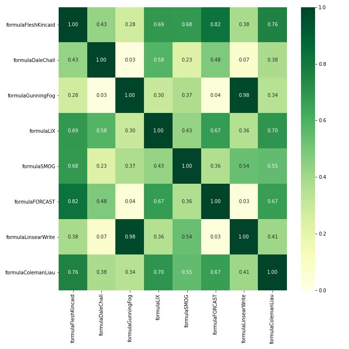
vi | Contents

References                                                              45

A Formulation of readability tests                                      53

B Word lists                                                            54

C Detailed statistics of readability metrics                             55
  C.1 Airline tweets . . . . . . . . . . . . . . . . . . . . . . . . . . 55
  C.2 IMDb reviews . . . . . . . . . . . . . . . . . . . . . . . . . . 67
LIST OF FIGURES | vii
List of Figures
1 Sentiment analysis methodologies . . . . . . . . . . . . . . . 11
2 Overall thesis process and code structure . . . . . . . . . . . . 17
3 Data cleaning methodology . . . . . . . . . . . . . . . . . . . 20
4 Word2Vec model overview . . . . . . . . . . . . . . . . . . . 21
5 Hidden layer and word embedding matrix . . . . . . . . . . . 21
6 Target and context words in the skip-gram model . . . . . . . 22
7 Target and context words in the CBOW model . . . . . . . . . 23
8 Confusion matrix . . . . . . . . . . . . . . . . . . . . . . . . 25
9 Example ROC curve . . . . . . . . . . . . . . . . . . . . . . 26
10 ROC curve and AUC . . . . . . . . . . . . . . . . . . . . . . 36
11 Sensitivity of balanced accuracy to corpus size . . . . . . . . 37
12 Airline tweets, positive sentiments, correlations between picked
metrics . . . . . . . . . . . . . . . . . . . . . . . . . . . . . 58
13 Airline tweets, negative sentiments, correlations between picked
metrics . . . . . . . . . . . . . . . . . . . . . . . . . . . . . 59
14 Airline tweets, correlations between readability formulae . . . 60
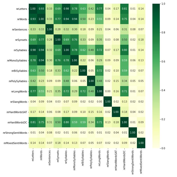
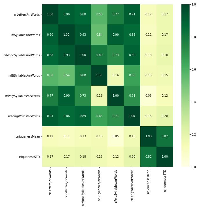
15 Airline tweets, correlations between base metrics . . . . . . . 61
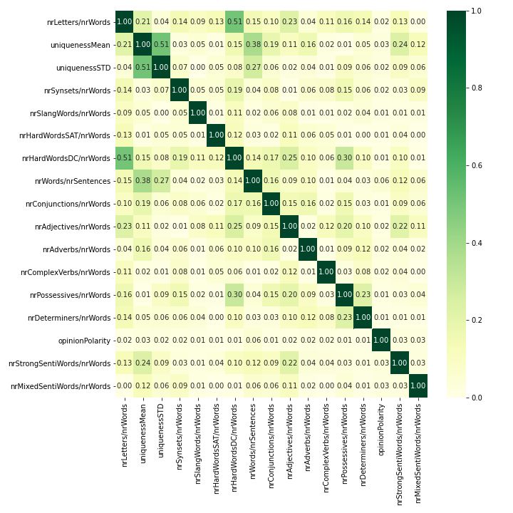
16 Airline tweets, correlations between lexical metrics . . . . . . 62
17 Airline tweets, correlations between semantic metrics . . . . . 63
18 Airline tweets, correlations between syntactic metrics . . . . . 64
19 Airline tweets, correlations between POS metrics . . . . . . . 65
20 Airline tweets, correlations between sentiment metrics . . . . 66
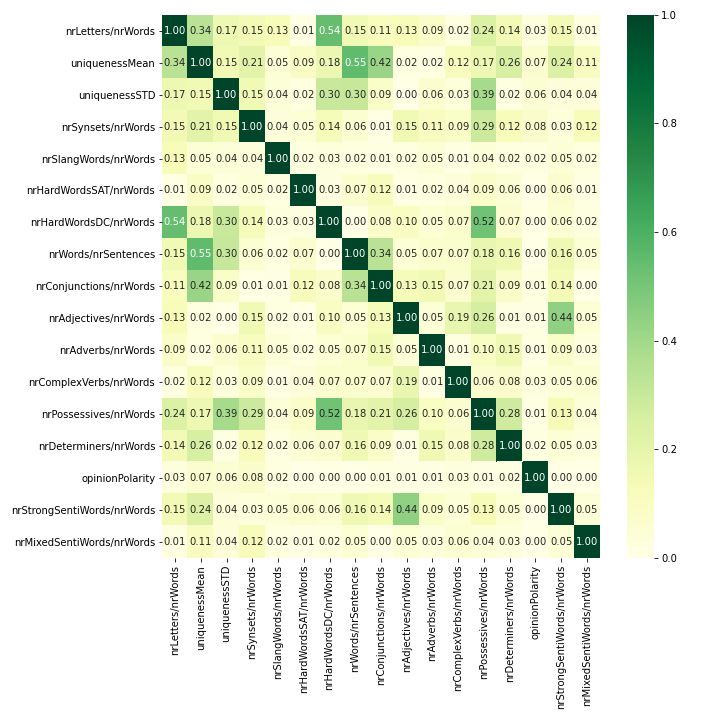
21 IMDb reviews, positive sentiments, correlations between picked
metrics . . . . . . . . . . . . . . . . . . . . . . . . . . . . . 69
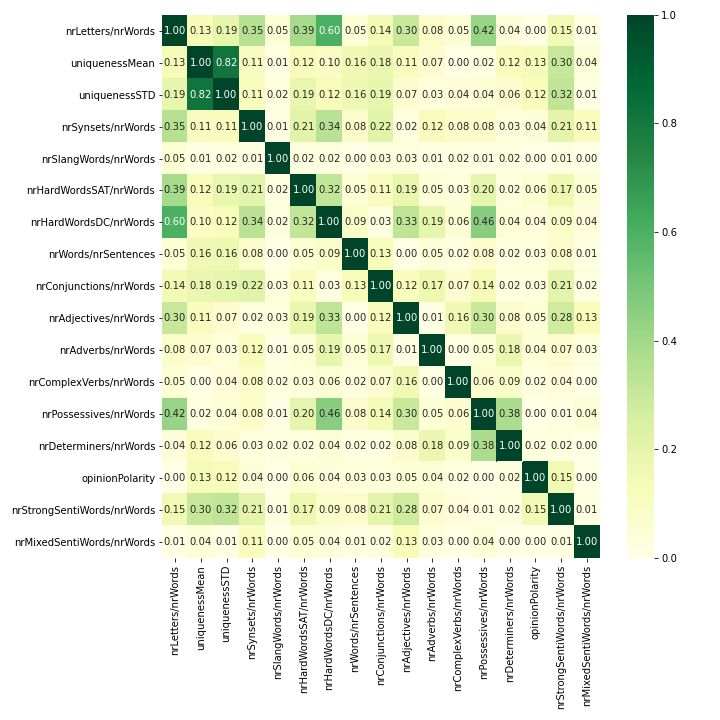
22 IMDb reviews, negative sentiments, correlations between picked
metrics . . . . . . . . . . . . . . . . . . . . . . . . . . . . . 70
23 IMDb reviews, correlations between readability formulae . . . 71
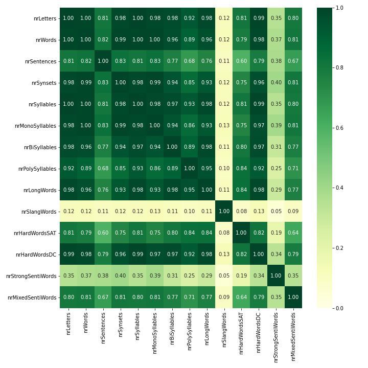
24 IMDb reviews, correlations between base metrics . . . . . . . 72
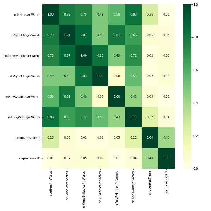
25 IMDb reviews, correlations between lexical metrics . . . . . . 73
26 IMDb reviews, correlations between semantic metrics . . . . . 74viii | LIST OF FIGURES 27 IMDb reviews, correlations between syntactic metrics . . . . . 75 28 IMDb reviews, correlations between POS metrics . . . . . . . 76 29 IMDb reviews, correlations between sentiment metrics . . . . 77
LIST OF TABLES | ix

List of Tables

 1    Assessment of Flesch-Kincaid reading ease score .          .   .   .   .   .   .    5
 2    Commonly used readability formulae and metrics .           .   .   .   .   .   .    6
 3    Word embedding techniques . . . . . . . . . . . .          .   .   .   .   .   .    9
 4    Overview of datasets . . . . . . . . . . . . . . . .       .   .   .   .   .   .   19
 5    Overview of software and libraries . . . . . . . . .       .   .   .   .   .   .   28
 6    Overview of implemented W2V hyperparameters .              .   .   .   .   .   .   29
 7    Longlist of base readability metrics . . . . . . . . .     .   .   .   .   .   .   30
 8    Derived readability metrics and final picks . . . . .      .   .   .   .   .   .   32
 9    Confusion matrix and balanced accuracy . . . . . .         .   .   .   .   .   .   35
 10   Estimation of β-values for the logistic regression .       .   .   .   .   .   .   38
 11   Variance inflation factor per metric . . . . . . . . .     .   .   .   .   .   .   39
 12   Definitions of readability formulae . . . . . . . . .      .   .   .   .   .   .   53
 13   Words used for clustering vectors and slang metric         .   .   .   .   .   .   54
 14   Airline tweets, detailed statistics per metric . . . .     .   .   .   .   .   .   56
 15   Airline tweets, detailed statistics per metric (cont.) .   .   .   .   .   .   .   57
 16   IMDb reviews, detailed statistics per metric . . . .       .   .   .   .   .   .   67
 17   IMDb reviews, detailed statistics per metric (cont.)       .   .   .   .   .   .   68
x | List of acronyms and abbreviations

List of acronyms and abbreviations
ABSA Aspect-Based Sentiment Analysis

ALBERT A Lite BERT

AUC Area Under Curve

BERT Bidirectional Encoder Representations from Transformers

BiLSTM Bidirectional Long Short-Term Memory

CBOW Continuous Bag of Words

CLM Contextual Language Models

CNN Convolutional Neural Network

CRNN Convolutional Recurrent Neural Network

ELMo Embeddings from Language Models

FPR False Positive Rate

GloVe Global Vectors

GRU Gated Recurrent Unit

IMDb Internet Movie Database

LSTM Long Short-Term Memory

MRC Machine Reading Comprehension

NLP Natural Language Processing

NLU Natural Language Understanding

NN Neural Network

PMI Pointwise Mutual Information

POS Part of Speech

QA Question Answer

RNN Recurrent Neural Network
List of acronyms and abbreviations | xi

RoBERTA Robustly Optimized BERT pretraining Approach

ROC Receiver Operating Characteristic

TF-IDF Term Frequency - Inverse Document Frequency

TNR True Negative Rate

TPR True Positive Rate

ULMFiT Universal Language Model Fine-tuning

VADER Valence Aware Dictionary and sEntiment Reasoner

VIF Variance Inflation Factor

W2V Word2Vec
Introduction | 1

Chapter 1

Introduction

1.1      Background
Since the early 20th century, linguists have developed a myriad of readability
tests to assess the ease with which a written text can be read and understood
by human beings [1]. A text is tested by inputting various metrics pertaining
to it into a formula to calculate an overall readability score. A few examples of
such readability metrics are the average length of the words in a text, as well
as the perceived difficulty of the words. The resulting score is then assessed
against a scale which corresponds to the level of education or age needed for
a reader to understand the text.
     Over the years, these formulae have been honed to improve statistical
significance, and our knowledge of the contexts in which the formulae work, as
well as which metrics should be included therein, has improved. Nevertheless,
the primary focus of these readability metrics has been on assessing the human
understanding of texts. With the recent advent of Natural Language Processing
(NLP) techniques that allow computers to analyse text, this provides an
interesting opportunity to assess whether readability metrics also can be used
to inform on the ease with which machines understand texts.
     An area which could be of particular interest for such research is sentiment
analysis. This is a rich subfield of NLP and concerns itself with identification
and quantification of affective states by means of machine learning [2]. To
date, most research in the field has centred on supervised learning, in which
texts must first be manually labelled with sentiments to provide a model with
training inputs. The trained model can then be used to classify unlabelled texts
from a hitherto unseen dataset, be it from the same text domain or a different
one. In the latter case, researchers are using so-called transfer learning.
2 | Introduction
Labelling data for supervised learning can be resource- and time intensive,
and transfer learning is not always possible if the target domain is too
dissimilar to the domain on which the model was trained. In such cases, a
possible fallback option is to instead use unsupervised learning. This method
allows the machine learning model to find patterns in unlabelled data by
trying to infer an a priori probability distribution. In both supervised and
unsupervised sentiment analysis, a machine crafts an understanding of the
sentiments expressed in the texts. However, unsupervised learning reduces
the need for human intervention and manual overlay vis-à-vis supervised
learning. It therefore relies more heavily on the inner workings - and thus
the ’understanding’ - of the machine, which is especially interesting for the
purposes of this paper.
In 2013, Tomas Mikolov at Google released two papers [3], [4] specifying a
new technique for NLP called Word2Vec (W2V). The algorithm uses a Neural
Network (NN) to create word embeddings, which represent words as vectors
based on their semantic and syntactic similarity. This technique has since been
widely adopted in sentiment analysis [5], [6], [7]. A key strength when used
for the purposes of unsupervised learning is that the technique has limited need
for human a priori knowledge and is instead more dependent on the dataset on
which it is trained, again meaning that it relies more on the machine than the
human. Unsupervised learning using word embeddings could therefore be an
interesting way to model a machine’s understanding of a text, and readability
metrics could potentially be used to predict the accuracy thereof.
1.2 Problem statement and scope
This paper investigates whether the readability metrics commonly used to
assess the ease with which humans read and understand texts also can be
used to inform on the ease with which machines do so. More specifically, the
machine assessed in this paper implements an unsupervised sentiment analysis
model using word embeddings. The research question for this paper is:
To what extent do human readability metrics predict accuracy when using
word embeddings for unsupervised sentiment analysis?Introduction | 3
The proposed subject area fills a gap in the current scientific literature as it
makes explicit a potential linkage between two existing bodies of research:
readability and sentiment analysis. It may therefore provide an abstract
understanding of the connection between human and machine comprehension
(of sentiments), including their similarities and differences.
Furthermore, this line of research may provide further insight into the
contexts in which unsupervised sentiment analysis performs well, when using
word embeddings to conduct the analysis. Should datasets with high (or
low) values for certain readability metrics consistently predict accuracy to
a high degree, this could indicate that particular qualities are desirable, or
even required, to be able to conduct this type of sentiment analysis. This is
of particular interest as neither supervised learning, nor transfer learning, are
feasible in all contexts, and, despite this, research into unsupervised sentiment
analysis is relatively sparse.
It should be noted that in order to assess the accuracy of a sentiment
analysis model, one must have access to labels with the correct sentiments.
However, an approach cannot be considered unsupervised if it actually utilises
these labels for anything besides the testing of its final predictions. Simply
put, an unsupervised model should not be able to ’peak’ at the correct answers
during training, which means that the labels cannot be used for picking the
right data cleaning methodologies or for tuning of hyperparameters. As such,
the unsupervised model in this thesis will rely heavily on established practices
based on previous research, making it both more generic and more general.
Several word embedding technologies exist. This paper focuses on W2V
for reasons specified in Section 2.2. Similarly, a plethora of readability metrics
exist and this paper focuses on those most commonly used. This will be
further elaborated upon in Section 2.1. Moreover, the readability metrics
are included in their base form, as is common in the literature. This means
that no transformations are made to them, such as taking the square root or
logarithm. Doing so would provide further convolution to analysis which is
likely unwarranted (although of potential interest for future work).Theory and literature review | 5
Chapter 2
Theory and literature review
2.1 Readability
The readability of a text is quantitatively assessed by extracting metrics from
the text and plugging them into a formula to calculate a score. For instance, one
of the first assessments developed in the field - the Flesch-Kincaid reading ease
score [8] - is calculated with the formula below. The resulting score ranges
from 0 to 100 and is used together with the information in Table 1 to assess
the text.
nrWords nrSyllables
206.835 − 1.015 − 84.6
nrSentences nrWords
Table 1 – Assessment of Flesch-Kincaid reading ease score
Score School level (US) Description
100-90 5th grade Very easy to read
90-80 6th grade Easy to read
80-70 7th grade Fairly easy to read
70-60 8th to 9th grade Plain English
60-50 10th to 12th grade Fairly difficult to read
50-30 College Difficult to read
30-10 College graduate Very difficult to read
10-0 Professional Extremely difficult to read6 | Theory and literature review
Most readability formulae were invented for either educational or military
purposes and are commonly used to assess school textbooks, as well as military
manuals, health service messages, insurance policies and newspaper articles.
In fact, several U.S. states have readability statues for their insurance policies,
commonly requiring the policies to score well on the Flesch-Kincaid test
[9]. All formulae have been calibrated and validated against the results from
reading comprehension tests, in which people must read a text and answer
questions pertaining to it. The most common reading comprehension test is
the McCall-Crabbs test [10].
Table 2 provides an overview of the most common and widely cited
formulae, specifying the year a formula was introduced, the name with which it
is commonly referred, the base readability metrics included in the formula and
a reference to the scientific paper where the formula was first presented. For
further detail on the extract structure of the formulae, please see Appendix A.
To define difficult words in the Dale-Chall formula, the authors use a list of
words easily recognised by 80% of fourth-grade students [11]. If a word cannot
be found in that list, it is considered difficult. Moreover, monosyllables are
defined as words with one syllable, bisyllables are words with two syllables,
and polysyllables are words with three or more syllables. Long words are
defined as words with more than six letters.
Table 2 – Commonly used readability formulae and metrics
Year Formula Metrics Ref.
1948 Flesh-Kincaid nrWords, nrSentences, nrSyllables [8]
1948 Dale-Chall nrWords, nrSentences, nrDifficultWords [11]
1952 Gunning fog nrWords, nrSentences, nrPolySyllables [12]
1968 LIX nrWords, nrSentences, nrLongWords [13]
1969 SMOG nrSentences, nrPolySyllables [14]
1973 FORCAST nrWords, nrMonoSyllables [15]
1974 Linsear Write nrSentences, nrMonoSyllables, [16]
nrBiSyllables, nrPolySyllables
1975 Coleman-Liau nrWords, nrSentences, nrLetters [17]Theory and literature review | 7
The above metrics are typically divided by one another in the formulae. This
means that the formulae implicitly derive other, composite readability metrics.
For instance, by dividing the number of letters in a text by the number of words,
one can produce the average length of the words in that text. Such metrics can
broadly be categorised into three analytical areas:
• Lexical metrics: Pertaining to the structure and morphology of words,
for instance the average word length
• Semantic metrics: Pertaining to the meaning of words, for instance the
perceived difficulty of the words
• Syntactic metrics: Pertaining to the use of words in sentences, for
instance the average sentence length
The Flesch-Kincaid and Dale-Chall formulae have since their introduction
been updated in 1975 [18] and 1995 [19], respectively. In so doing, coefficients
in the formulae were updated, but no new metrics were included, resulting in
improvements to the correlations between formula scores and the results of
reading comprehension tests. Flesch-Kincaid currently has a correlation of
0.91, whereas Dale-Chall has the highest correlation of all formulae at 0.93.
In 2000, the ATOS reading ease formula [1] was published, based on
extensive research spanning reading records from 950 thousand books. The
researchers concluded that the most reliable metrics were the average word
length, the average sentence length and the difficulty of the words. In addition
to these more traditional metrics, Golub’s syntactic density score [20] instead
uses ten different syntactic metrics. This score predominantly focuses on Part
of Speech (POS) tags, which classify words into different types of nouns, verbs
or adjectives, amongst others.
In recent years, researchers have started using advanced machine learning
techniques to identify additional metrics that can be used to predict text
readability. For instance, [21] specifies a lexico-semantic measure of language
model perplexity as a potential metric candidate. Moreover, [22] identifies
various metrics pertaining to lexical chains. Lastly, when examining the
grammatical structure of a text using POS tags, the height of the corrresponding
parse tree has been found to be a potential metric candidate [23]. Nevertheless,
several of these new metrics are complicated to extract and not always
intuitively understood by human beings.8 | Theory and literature review
2.2 Vectorisation
A corpus is a structured set of texts (or documents). To analyse corpora
using machine learning algorithms, one must first vectorise their vocabularies.
One way of doing this is by means of Term Frequency - Inverse Document
Frequency (TF-IDF) [24]. This metric reflects how important a term (or word)
is to a specific document in a corpus. It increases if a word appears many times
in a particular document and decreases if it occurs across many documents in
the corpus. It is calculated as:
tfidf(t, d, D) = tf(t, d) ∗ idf(t, D)
The term frequency tf(t, d) is defined as the number of times that the term t
occurs in a document d divided by the number of times that the other terms
occur in that document:
ft,d
tf(t, d) = P
t0 ∈d ft0 ,d
The inverse document frequency idf(t, D) is defined as the number of documents
N in a corpus divided by the number of documents where the term t appears:
N
idf(t, D) = log
|{d ∈ D : t ∈ d}|
TF-IDF provides numerical representations of word-document combinations.
The metric is therefore primarily used in recommender systems. Indeed,
previous research has shown that TF-IDF is used in 83% of recommender
systems [25]. For the purposes of the analysis in this paper, the mean and the
standard deviation across all the TF-IDF scores of words in a given document
are calculated to produce a metric specifying the uniqueness of the words in
that document.
Instead of producing word-document representations, one can use word
embeddings such as W2V to produce word-level vectors. The vectors resulting
from such techniques can be used to measure and find semantic similarities
between words. One such measurement is that of cosine similarity:
A·B
cos θ =
||A|| ||B||Theory and literature review | 9
Cosine of the angle between two word vectors, A and B, is bounded between
-1 and 1. A value of -1 indicates that the words are opposites, 0 means that
they are unrelated and 1 that they are exactly the same. A given word vector
can thus be used to find other, similar (or dissimilar) word vectors.
In addition to the previously mentioned W2V, five more word embedding
techniques currently exist: Global Vectors (GloVe), FastText, Universal Language
Model Fine-tuning (ULMFiT), Embeddings from Language Models (ELMo),
and Bidirectional Encoder Representations from Transformers (BERT). These
are illustrated in Table 3.
Table 3 – Word embedding techniques
Technique Representation Context vectors Method Ref.
Word2Vec Words No NN [3]
GloVe Words No Frequency [26]
FastText Sub-words No NN [27]
ULMFiT Words Yes LSTM [28]
ELMo Characters Yes Bi-LSTM [29]
BERT Sub-words Yes Transformers [30]
Google’s W2V is a NN model which tries to predict word co-occurrences
based on their contexts, resulting in a vector representation per word. As it
is of particular focus for this paper, further elaboration of its inner workings is
provided in Section 3.3.1.
Stanford’s GloVe model is similar to W2V in the sense that it also provides
vector representations at the word-level. However, while W2V is a predictive
NN, GloVe is a frequency-based model which constructs a co-occurence
matrix of words and documents based on how often words appear in specific
contexts. This matrix is factorised to produce a low-dimension representation
to save computational power. Both GloVe and W2V tend to produce similar
results for many tasks, although the latter has seen more widespread adoption
and add-ons over time.
Facebook’s FastText is essentially an extension of W2V. Whereas W2V
uses words as its lowest level of atomicity, FastText instead uses subsets of
words, or subwords. These substring representations are particularly useful
for out-of-vocabulary issues, namely in cases where one tries to feed a new
word to a model pre-trained on a corpus which does not contain that particular
word. By instead representing words as combinations of substrings, the model10 | Theory and literature review
will recognise previously unseen words. Moreover, the size of the vocabulary
can also be reduced.
While the aforementioned word embedding techniques only create one
vector representation per word in a corpus, ULMFiT, ELMo and BERT all
allow the vector representations of words to vary depending on the context of
the word. As such, a word such as ’bank’ will have a different meaning and
vector depending on if it is in a context pertaining to finance vis-à-vis rivers.
Such models are also called Contextual Language Models (CLM) [31].
CLMs come pre-trained on very large corpora such as English Wikipedia.
Nevertheless, they can be fine-tuned using new data. The extent of the fine-
tuning is manually chosen to allow a share of model parameters to remain
locked and the remaining parameters to be updated using new data. This share
is chosen based on the new corpus size and available computational power.
Generally, word embedding techniques perform better if trained on larger
corpora. For instance, the first W2V paper [3] demonstrated that reductions
in corpus size impacted model accuracy significantly. Small corpora or
limited access to hardware therefore necessitate extensive use of a pre-trained
CLM with limited fine-tuning. Nevertheless, these pre-trained models tend
to perform well on previously unseen data due to already having been trained
on large corpora. Should the aforementioned limitations not be applicable,
CLMs can essentially be entirely re-trained using new data and only use the
pre-training for initial model weights (as opposed to randomised weights).
ULMFiT represents words using a Long Short-Term Memory (LSTM)
model and ELMo represents characters using a Bidirectional Long Short-Term
Memory (BiLSTM) model, both of which are NN variations with additional
memory. However, bidirectionality in ELMo is only ensured by concatenating
left-to-right and right-to-left information, meaning that it does not take into
account both directions simultaneously. Google’s BERT accounts for this
by instead using the recently developed transformer technology on subwords.
A transformer is a deep learning model which uses autoencoders and an
attention-mechanism which dedicates more computing power to small but
important parts of the data. BERT therefore mimics how a brain provides
attention to tasks.
Context-varying vectors perform in line with humans when used for
sentiment analysis tasks [31]. Nevertheless, they tend to be resource intensive,
requiring advanced hardware to run over long periods of time. Furthermore,
their results are not always well-understood [32], [33] and risk being hard to
analyse. Therefore, for the purposes of this thesis, W2V is deemed a more
appropriate method for vectorisation.Theory and literature review | 11
It should also be noted that sentence-level embedding techniques have been
developed leveraging the aforementioned technologies. Such embeddings
include Doc2Vec [34], SentenceBERT [35], InferSent [36], and Universal
Sentence Encoder [37]. These are often used for recommendation systems
and topic modelling and are therefore not in scope for this paper.
2.3 Sentiment analysis
Sentiment analysis is used to identify and quantify affective states and opinions
[2]. Such analyses can range from simple opinion polarity identification, to
more complex methodologies in which not only an opinion is extracted but
also the topic corresponding to that opinion. The latter is called Aspect-Based
Sentiment Analysis (ABSA) or feature-level sentiment analysis.
In the simplest and most common form of analysis, sentiments are binarily
classified as either positive or negative. More advanced models also attempt to
classify sentiments as neutral [38], [39], or on a scale [40], [41]. Other models
instead try to detect sarcasm [42], [43] or emotions such as anger and disgust
[44]. For the purposes of this paper, the sentiment analysis is specified as a
binary polarity classification.
Figure 1 illustrates the different methodologies which can be used for
sentiment analysis. This paper focuses on unsupervised sentiment analysis.
Figure 1 – Sentiment analysis methodologies12 | Theory and literature review
Sentiment analysis can use either machine learning or a rule-based approach.
The former typically uses supervised learning, which feeds a vectorised corpus
and labelled data into an algorithm. Examples of such algorithms are standard
models such as Naïve Bayes, Maximum Entropy, Support Vector Machines
and ensemble classifiers [45]. Recent years have also seen the emergence
of NN models such as the Recurrent Neural Network (RNN), including
variations thereon such as LSTM, BiLSTM and Gated Recurrent Unit (GRU).
Moreover, some models utilise a Convolutional Neural Network (CNN) or a
Convolutional Recurrent Neural Network (CRNN) [46].
More advanced supervised sentiment analysis methods use variations on
the previously mentioned BERT to conduct sentiment analysis [47], [48]. This
word embedding technique has been complemented with supervised learning
capabilities and various adjustments have been made to the architecture,
resulting in variants such as Robustly Optimized BERT pretraining Approach
(RoBERTA) [49] and A Lite BERT (ALBERT) [50], amongst others. These
methods are considered the current state-of-the-art in supervised sentiment
analysis and score in line with human beings on sentiment classification tasks.
It should be noted that mislabelling of sentiments is common due to the
lack of a common interpretative standard. Inter-rater agreement is estimated
at approximately 80% [51], putting an upper bound on the potential accuracy
of supervised sentiment analysis methods. Moreover, labelling is not always
possible due to time- and resource constraints. Nevertheless, once a supervised
sentiment analysis model has been trained on a corpus it can also potentially
be used to classify documents in another corpus, using transfer learning.
Unsupervised learning methods instead use statistical inference based on
a priori assumptions. While such methods are relatively rare, some examples
exist. For instance, [52] specifies a model using Pointwise Mutual Information
(PMI) between words, calculated based on the probability that the words co-
occur. The orientation of a phrase is based on comparing the PMI of its
constituent words with the sentiment words ’excellent’ and ’poor’ and picking
the sentiment word with the highest PMI. In a more recent paper [53], W2V
is used to vectorise the corpus. To then classify the sentiment of a given
observation, the cosine similarity between the words in an observation and
the words in a pre-defined list of sentiment words is calculated. A similar
approach is used in this report.
It should be noted that several authors refer to their methods as being
’unsupervised’, despite using rule-based approaches. See, for instance, [54],
[55]. While it is correct that such approaches do not require labels, they do
not use machine learning techniques. They rather rely on rules and lexicons,Theory and literature review | 13
which therefore should be reflected in the terminology with which they are
referred. Nevertheless, some models [56], [57] combine such rule-based
approaches with statistical inference, for instance using W2V. Such models
could be considered ’hybrids’.
Rule-based approaches use lexicons to derive sentiments. Simpler variants
only use a sentiment lexicon to do so, mapping words to sentiment scores
from the lexicon and calculating an overall score across all words. More
advanced models use a lexicon of POS tags with a lexicon of synsets to derive
sentiments. POS tags are used to craft an understanding of how the text is
structured based on grammatical rules. The synsets are used to understand
the polarity of the underlying words. Combined, the algorithm can derive
an opinion and its context, taking into account, for instance, negations and
modifying phrases. A recent examples of a high-performing rule-based model
is Valence Aware Dictionary and sEntiment Reasoner (VADER) [58].
Synsets are hierarchical structures of hypernyms and hyponyms based
on the semantic similarities of words. For instance, the word ’colour’ is a
hypernym to the word ’red’, which in turn is a hyponym to the word ’blue’.
However, ’blue’ might also mean ’to feel down’ and this interpretation is not
related to the word ’red’. All such interpretations and hierarchies are stored in
different synsets. By combining the contextual information of the grammatical
rules, modern lexical approaches try to infer which synset should be used, and
as such the interpretation and underlying polarity of the word. Two commonly
used lexicons of synsets are WordNet [59] and SentiWordNet [60].
A key strength of rule-based approaches is that they can pick up on
contextual information, unlike many unsupervised methods. However, there
are two major disadvantages to using rule-based approaches. Firstly, they are
often dependent on people using grammar correctly, which need not be the
case in corpora such as collections of tweets. In fact, a common problem
in NLP using online corpora is that the use of language is filled with slang
and improper use of language [61]. Secondly, they are heavily reliant on
their underlying lexicons, which are pre-defined by humans and therefore
sensitive to errors of judgement. Moreover, the lexicons must be rich enough
to appropriately cover a corpus’ words and meanings. Nevertheless, both rule-
based and unsupervised approaches bypass the necessity of having labels.
A potential linkage between readability metrics and sentiment analysis
results has previously been briefly explored in [62]. The paper examines
corpus dimensions for two datasets and then conducts sentiment analysis using
these datasets. However, the authors make no explicit mapping between corpus
dimensions and the results from the sentiment analysis on the two datasets.14 | Theory and literature review
They note that a potential connection is likely, constituting grounds for future
work.
2.4 Machine reading comprehension
Natural Language Understanding (NLU) is a subfield of NLP focused on
inference and reasoning based on text inputs. A key focus area therein is
the field of Machine Reading Comprehension (MRC), which concerns itself
with how machines extract information and infer meaning from texts [31].
It is tested in the same way as reading comprehension in humans is tested,
namely by letting the machine (or human) read a text and then asking questions
pertaining to it. These questions should then be answered by the machine or
human being. Such Question Answer (QA) tests can take the following forms:
• Cloze-style: Filling in the blanks
• Multi-choice: Picking the right choice(s)
• Span extraction: Extracting the relevant snippets of text and reciting
them
• Free text answers: Producing free-form sentences based on the text
This means that, in addition to analysing the text, MRC models should also
be able to understand questions pertaining to the text, infer answers thereto
and provide these in a structured format. For such tasks, CLMs such as BERT
have become dominant due to the high accuracy they receive on analytical
tasks [31].
If combined with QA capabilities, a sentiment analysis model falls into
the category of MRC. However, the model built as part of this paper does not
include such capabilities and instead focuses solely on analysis. Simply put,
the question the model should answer is constant - define the sentiment of the
text. Nevertheless, the sentiment analysis model designed in this paper does
not recite what is written in a text, but is rather inferring the sentiment of the
author. It is therefore inferring things beyond the text, which in itself is a
challenging and interesting analytical task.
To solve problems, more advanced MRC models require a plethora of
skills such as elaboration and inference of causal or spatiotemporal relations.
Previous research [63] has examined the correlation between the number of
skills required for a MRC model to solve tasks from different datasets andTheory and literature review | 15 the readability metrics of the datasets. Examples of such metrics include the average length of words, the average length of sentences and prevalence of modifiers and adverbs. Results indicated that readability of MRC datasets did not directly affect the difficulty of the tasks which the datasets were designed to test. The paper did not look into the effects that the readability metrics had on the inner functionality of a model, nor its results.
Methodology | 17

Chapter 3

Methodology

3.1      Process
Figure 2 illustrates the process required to produce and evaluate the results in
this thesis. It is also illustrative of how the code is structured at a high level.

               Figure 2 – Overall thesis process and code structure
18 | Methodology
While the following sections go into greater detail on the process elements,
a high-level description of the diagram is provided here. Datasets are first
chosen and cleaned using standard methodologies. After picking W2V
hyperparameters, the model is trained on the cleaned data. Afterwards, the
trained model is used to create two clustering vectors that help delineate and
predict the positive and negative sentiments. Predictions are then compared
to the correct labels to create a dichotomous outcome variable per sentiment,
representing whether the W2V model predicted the sentiments correctly.
In parallel to the W2V training and prediction, readability metrics are
extracted based on a pre-defined longlist of candidate metrics. A shortlist of
these metrics is then created based on an assessment of the correlation between
the metrics, as well as based on their potential explanatory value. Lastly,
a logistic regression is run, using the aforementioned dichotomous outcome
variable as dependent and the readability metrics as independent.
3.2 Data
To ensure reliability and validity of data, as well as generalisability of results,
this paper examines two high-quality datasets that span different domains:
tweets directed at airlines [64] and Internet Movie Database (IMDb) reviews
[65]. These datasets are both widely used for sentiment analysis research [66],
[67], [68] due to their richness and the high accuracy of the labels. Table 4
provides an overview of the datsets, including their domain, the time period
of the data, the labelling methods, the amount of observations and how these
are split across positive and negative sentiments, respectively.
Lastly, an overview is provided of the estimated age required to understand
the dataset contents, based on results from the aforementioned readability
formulae, in the order they were introduced historically. As can be noted
from the readability tests, the tweets require a minimum age of approximately
11 to be understood on average, whereas people aged 14 and above should
understand the IMDb reviews. It should also be noted that results from the
formulae correlate highly. For more details, please refer to Appendix C.Methodology | 19
Table 4 – Overview of datasets
Airline tweets IMDb reviews
Domain Twitter Movie reviews
Time period February 2015 June 2011
Labelling Externally assesed Self-provided
Total observations 8 897 50 000
Positive sentiments 17% 50%
Negative sentiments 83% 50%
Flesh-Kincaid 11-12 13-15
Dale-Chall 14-16 16-18
Gunning-Fog 7-11 14-17
SMOG 7-11 14-17
FORCAST 14-17 14-17
Linsear-Write 7-11 17+
Coleman-Liau 11-14 11-14
The airline tweets have been manually labelled by external reviewers. As
previously mentioned in Section 2.3, human beings are not always in full
agreement on how text should be interpreted. Nevertheless, the airline tweets
dataset also provides a confidence score, which estimates how confident
labellers are about their sentiment classification. To alleviate concerns related
to manual labelling, only observations are included where the certainty of the
labels has been marked as 100%.
Conversely, sentiments in the IMDb reviews are self-provided on a scale
from one to ten, where lower scores signify that movie watchers did not find
the film good. Based on these scores, sentiments have been automatically
extracted, denoting scores between one and four as negative sentiments and
scores between seven and ten as positive sentiments. It should also be noted
that observations in the IMDb dataset have been explicitly picked to ensure
perfect balance between positive and negative sentiments, whereas the airline
tweets have been picked at random and are therefore skewed towards negative
sentiments.20 | Methodology
The labels are used to test the accuracy of the predictions of the W2V model.
Incorrect labels therefore add noise to the evaluation of the W2V results and
as such to the dependent variable in the regression model. By including
two datasets with different labelling approaches, concerns pertaining to the
adequacy of labelling are alleviated. Furthermore, should the explanatory
power of the regression model be high, this indicates that the noise is likely
not detrimental to the findings.
Figure 3 illustrates the data cleaning methodology used. It should be
noted that many of the previously cited supervised sentiment analysis models
commonly apply additional data cleaning methodologies. These include the
removal of common words and stemming to reduce conjugated words into
their base form. This is instead handled by the W2V model, where needed.
As such, the data cleaning approach below minimises information loss while
reducing noise for the W2V model.
Figure 3 – Data cleaning methodology
By tokenising the data, each word in a sentence is turned into its own unit to be
used as input in the W2V model. All tokens are then turned into lowercase to
no longer distinguish words by case. All hashtags, usernames and hyperlinks
are then removed as they provide noise to the model. Lastly, all remaining
non-alphabeticals are removed to further reduce noise.
3.3 Models
3.3.1 Word2Vec
The W2V model is a neural network that has one hidden layer with linear
neurons and an output layer which uses a softmax classifier, explained in
detail further below. The Continuous Bag of Words (CBOW) implementation
is used in this paper, as it generally performs better on smaller datasets [3].
Nevertheless, the more intuitively understood skip-gram version is explained
first and an explanation is then provided on how the CBOW differs from it.
Figure 4 illustrates an example of a skip-gram W2V with a 10 000 word
vocabulary and 300 vector dimensions.Methodology | 21
Figure 4 – Word2Vec model overview
Network inputs are represented as one-hot vectors, meaning that they have the
same length as the vocabulary and each position in a vector corresponds to a
unique word. A specific word in the vocabulary is represented by zeros in all
positions except one particular position in which it has a one. The neurons
in the hidden layer are the dimensions used for the word embeddings. The
hidden layer can be represented as a matrix where each row corresponds to a
word and each column to a dimension. This is illustrated in Figure 5.
Figure 5 – Hidden layer and word embedding matrix22 | Methodology
In neural networks, the output layer tends to be the primary focus, and
calibration of the hidden layer is simply a means to an end. In the W2V model,
the hidden layer constitutes a vectorisation of the input words, meaning that it
is, in fact, a matrix of word embeddings. As extracting these is the purpose
of running the model, the other model elements are discarded upon finalising
calibration. For instance, the rows in Figure 5 represent words, so one can
simply look-up a particular word in that table (an example word is highlighted
in blue) to extract its 300 dimensions and, as such, its vector representation.
Nevertheless, as with many other neural networks, the hidden layer is
calibrated to optimise a function in the output layer by using stochastic gradient
descent and backpropagation. In the case of the W2V model, the hidden layer
is calibrated to maximise the probability of getting words nearby the input
words. The skip-gram model uses one input word at a time, the target word, to
try to predict the context words surrounding it. Figure 6 illustrates this using
a context window of size 2.
Figure 6 – Target and context words in the skip-gram model
The total likelihood of getting context words, given the target words and the
hidden layer calibration, is expressed as:
T
Y Y
L(θ) = P (wt+j |wt ; θ) (1)
t=1 −m≤j≤m
To simplify the formula, the negative log-likelihood is calculated instead:
T
1 1X X
J(θ) = − log L(θ) = − log P (wt+j |wt ; θ) (2)
T T t=1 −m≤j≤mMethodology | 23
The probability in Equation 2 is expressed using a softmax function, denoting
wc the hidden layer context word vector and wt the target word vector:
exp (wc · wt )
P (wc |wt ) = P 0
(3)
w0 ∈V ocab exp (w · wt )
The dot product between the context word vector and the target word vector in
the numerator means that word similarities correspond to higher probabilities.
The denominator is a normalisation factor to ensure that all probabilities sum
to 100%. Re-examining Figure 4, one can note that the output layer has ten
thousand neurons, namely one neuron corresponding to a probability per word
in the vocabulary. Given a specific input (target) word and a context window,
the skip-gram model adjusts the hidden layer to maximise the values in the
output layer neurons that correspond to the specific context words. This means
that not all output neurons are in focus for each possible input vector, although
across all input vectors, all output neurons will be.
While the skip-gram model predicts context words given a target word, the
CBOW model instead predicts target words given a context. This is illustrated
in Figure 7.
Figure 7 – Target and context words in the CBOW model
Re-examining Figure 4, the CBOW model instead has several input vectors,
each being a one-hot vector corresponding to a specific context word. For
each such context, the hidden layer is adjusted to maximise the probability in
a single output neuron, corresponding to the target word.
During backpropagation for a specific target word, most rows in the hidden
layer will not be adjusted. Secondly, the softmax calculation of all probabilities
is computationally expensive. To account for this, the W2V model uses
negative sampling, in which only the target and context words, as well as a
few additional words are sampled and updated. Common words such as ’the’24 | Methodology
are downsampled to ensure that words with explanatory power are more likely
to be sampled. This provides significantly better performance with negligible
reduction in accuracy [4].
Having extracted the word embeddings, two sentiment clustering vectors
are created using the average of key word vectors in the vocabulary. For
instance, the vectors of words such as good, fantastic and amazing can be
averaged to create a new vector representing positive sentiments. Similarly,
words such as bad, awful and horrible can be used to create a negative
sentiment vector. Words in a given observation can then be compared to
these sentiment clustering vectors using their cosine similarity. The clustering
vector which is most similar to all the words in a given observation is used for
classification. The methodology to arrive at the clustering vectors is further
elaborated upon in Section 3.5.
Lastly, the data is split into two subsets based on the correct labels,
meaning that one dataset corresponds to all cases where the true labels are
positive, and one where the true labels are negative. For each subset, the results
from the sentiment classifier are then compared to the correct labels to arrive
at a dichotomous outcome variable per sentiment, in which ones represent a
correct prediction and zeros represent an incorrect prediction.
3.3.2 Logistic regression
Using the dichotomous variable from the previous section as the dependent
variable in a logistic regression (per sentiment), one can analyse the effects
that the independent variables, the readability metrics, have on the probability
of the W2V model predicting a given sentiment correctly. The dependent
variable is thus denoted Y and the probability of getting a correct prediction
given the independent variables p = P (Y = 1|Xn ). By assuming a linear
relationship between the log-odds of p and the independent variables, the
following relation is specified:
n
p X
log = β0 + βn Xn (4)
1−p i=1
This means that the odds of getting a correct prediction can be defined as:
n
p X
= exp (β0 + βn Xn ) (5)
1−p i=1Methodology | 25
Through algebraic manipulation one can derive the following:
exp (β0 + ni=1 βn xn,i )
P
P (yi = 1) = + i , where i ∼ i.d.d.(0, σ 2 ) (6)
1 + exp (β0 + ni=1 βn xn,i )
P
The β-values are estimated through iterative maximum likelihood estimation,
by making repeated adjustments until the likelihood no longer can be improved.
Upon converging on final β-values, the interpretation of the model is that a
unit increase in X increases (or decreases) the log-odds of Y being a correct
prediction by β, if β is positive (or negative). That is to say that a unit increase
in a readability metric increases the probability of the W2V model predicting
a specific sentiment correctly if the readability metric has a positive β.
3.4 Evaluation framework
The validity of the W2V model is evaluated by examining its confusion matrix,
which illustrates the relative distribution of true and false predictions:
Figure 8 – Confusion matrix
Accuracy measures the rate with which a model correctly predicts all observations
and is calculated using the following values from the confusion matrix:
Accuracy: T P +T N
T P +T N +F P +F N
Another two measurements of predictive power can be calculated from the
confusion matrix, to then be combined into the balanced accuracy metric:26 | Methodology
True Positive Rate (TPR): TP
T P +F N
True Negative Rate (TNR): TN
T N +F P
Balanced accuracy: T P R+T N R
2
If the dataset is inbalanced (for instance because there are significantly more
negative observations than positive, as often is the case with sentiments
online), a model can get high accuracy by simply only predicting negative
observations. Therefore, a more appropriate measurement to evaluate the
model is balanced accuracy. This measurement takes into account the degree
with which the model discriminates between negative and positive cases.
The W2V model is also evaluated by varying its discrimination threshold
and examining the rate with which its TPR increases in exchange for increases
in its False Positive Rate (FPR), defined as:
FPR: FP
T N +F P
This is done by creating a graph of the two rates, called a Receiver Operating
Characteristic (ROC) curve, illustrated by the green line in Figure 9.
Figure 9 – Example ROC curve
If TPR improves significantly in exchange for small increases in FPR, the
model is of high quality. ROC curves are typically complemented by calculating
the Area Under Curve (AUC) statistic, which quantifies the discriminatory
power of the model. As the curve gets closer to the upper left-hand corner,
AUC values approach 1, which signifies a model with perfect discrimination.
The dotted line signifies the model predicting at random and corresponds to
an AUC of 0.5.Methodology | 27
After running and evaluating the W2V model, the same should be done for
the logistic regression. As previously mentioned, after predicting sentiments,
each dataset is split into two subsets: one per true sentiment. Separate logistic
regressions are then run for each subset. Thus, each logistic regression tests
whether the readability metrics can predict W2V model results depending
on what the true sentiment is. Examining the confusion matrix in Figure 8,
one can note that the split of datasets into subsets corresponds to vertically
separating the matrix into two parts, splitting it in the middle based on the
real values in the matrix. This ensures that one regression tests the effects of
moving from FN to TP and the other regression tests the effects of moving
from FP to TN, thus testing the W2V model’s predictive power while adding
granularity to the analysis.
The validity of the logistic regression is evaluated by examining McFadden’s
Pseudo-R2 , which is calculated as follows:
log L(Mf ull )
R2 = 1 −
log L(M0 )
L(Mf ull ) is the likelihood function of the final model and L(M0 ) is the
likelihood function of the model without any independent variables, meaning
it is only an intercept. A value of 0 means that the model offers no explanatory
value, whereas figures above 0.2 are considered ’excellent fit’ [69]. Furthermore,
the β-values are tested for statistical significance at the 1% level using
heteroscedasticity-robust standard errors to ensure that they indeed offer
explanatory power. Variables are also tested for multicollinearity by examining
Pearson’s correlation coefficients and their Variance Inflation Factor (VIF),
which should be below three to ensure variances are accurate [70].
Lastly, to ensure reliability of the results, the methodology used for the
thesis is extensively documented, allowing another author to reproduce all
results. In particular, Section 3.5 details the experimental setup, including
the software and libraries used, as well as the choice of hyperparameters and
how algorithms are seeded.28 | Methodology
3.5 Experimental setup
3.5.1 Software and libraries
Execution time when running the W2V model on the largest dataset - the
IMDb reviews - remains below 5 minutes using a current generation, high-spec
personal computer. As such, there are no particular hardware requirements to
recreate the experimental setup.
Table 5 provides an overview of the software and libraries required to
reprocude the results. All results from the logistic regression in statsmodels
were validated by also running the regression in sklearn and STATA, which is
software used explicitly for statistical analysis. No discrepancies were found.
Table 5 – Overview of software and libraries
Software Description Version
Microsoft VS Code editor, used to write, run and 1.55.2
Code debug code
Anaconda Python distribution platform, used to 3.8.5
code solution
Library Description Version
Pandas Python data analysis library, used for 1.2.3
manipulating data in tables
NLTK Natural language toolkit, used for 3.6.2
tokenisation and synset extraction
Sklearn Machine learning library, used for 0.24.1
helper functions, correlations and VIF
Gensim Machine learning library, used for the 4.0.1
Word2Vec model
Statsmodels Statistics library, used for logistic 0.9.0
regression
Seaborn Visualisation library, used for 0.11.1
correlation matricesYou can also read