EVOLUTION AND PREDICTION OF LANDSCAPE PATTERN AND HABITAT QUALITY BASED ON CA-MARKOV AND INVEST MODEL IN HUBEI SECTION OF THREE GORGES RESERVOIR ...
←
→
Page content transcription
If your browser does not render page correctly, please read the page content below
sustainability

Article
Evolution and Prediction of Landscape Pattern and
Habitat Quality Based on CA-Markov and InVEST
Model in Hubei Section of Three Gorges Reservoir
Area (TGRA)
Lin Chu 1,2 , Tiancheng Sun 1,2 , Tianwei Wang 1,2, *, Zhaoxia Li 1,2 and Chongfa Cai 1,2
 1   Key Laboratory of Arable Land Conservation (Middle and Lower Reaches of Yangtze River) of the Ministry
     of Agriculture, Soil and Water Conservation Research Centre, Huazhong Agricultural University,
     Wuhan 430070, China; chulin@mail.hzau.edu.cn (L.C.); tiancheng_hzau@sina.com (T.S.);
     zxli@mail.hzau.edu.cn (Z.L.); cfcai@mail.hzau.edu.cn (C.C.)
 2   College of Resources and Environment, Huazhong Agricultural University, Wuhan 430070, China
 *   Correspondence: wangtianwei@webmail.hzau.edu.cn

 Received: 25 August 2018; Accepted: 19 October 2018; Published: 24 October 2018

 Abstract: The spatial pattern of landscape has great influence on the biodiversity provided by
 ecosystem. Understanding the impact of landscape pattern dynamics on habitat quality is significant
 in regional biodiversity conservation, ensuring ecological security guarantee, and maintaining
 the ecological environmental sustainability. Here, combining CA-Markov and InVEST model,
 we investigated the evolution of landscape pattern and habitat quality, and presented an explanation
 for variability of biodiversity linked to landscape pattern in Hubei section of Three Gorges Reservoir
 Area (TGRA). The spatial-temporal evolution characteristic of landscape pattern from 1990 to 2010
 were analyzed by Markov chain. Then, the spatial pattern of habitat quality and its variation in three
 phases were computed by InVEST model. The driving force for landscape variation was explored
 by using Logistic regression analysis. Next, the CA-Markov model was used to simulate the future
 landscape pattern in 2020. Finally, future habitat quality maps were obtained by InVEST model
 predicted landscape maps. The results concluded that, the overall landscape pattern has changed
 slightly from 1990 to 2010. Woodland, waters and construction land had the greatest variations
 in proportion among the landscape types. The area of woodland has been decreasing gradually
 below the average elevation of 140 m, and the area of waters and construction land increased sharply.
 Logistics regression results indicated that terrain and climate were the most influencing natural
 factors compared with human factors. The Kappa coefficient reached 0.92, indicating that CA-Markov
 model had a good performance in future landscape prediction by adding nighttime light data as
 restriction factor. The biodiversity has been declining over the past 20 years due to the habitat
 degradation and landscape pattern variation. Overall, the maximum values of habitat degradation
 index were 0.1188, 0.1194 and 0.1195 respectively, showing a continuously increasing trend from 1990
 to 2010. Main urban areas of Yichang city and its surrounding areas has higher habitat degradation
 index. The average values of habitat quality index of the whole region were 0.8563, 0.8529 and
 0.8515 respectively, showing a continuously decreasing trend. The lower habitat quality index mainly
 located in the urban land as well as the main and tributary banks of the Yangtze River. Under the
 business as usual scenario, habitat quality continued to maintain the variation trend of the previous
 decade, showing a reducing habitat quality index and an increasing area of artificial surface. Under
 the ecological protection scenario, the variation of habitat quality in this scenario represented reverse
 trend to the previous decade, exhibiting an increase of habitat quality index and an increasing area
 of woodland and grassland. Construction of Three Gorges Dam, impoundment of Three Gorges
 Reservoir (TGR), resettlement of Three Gorges Project and urbanization were the most explanatory
 driving forces for landscape variation and degradation of habitat quality. The research may be useful

Sustainability 2018, 10, 3854; doi:10.3390/su10113854                    www.mdpi.com/journal/sustainability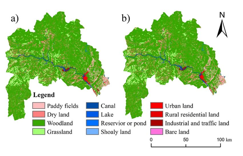
Sustainability 2018, 10, 3854                                                                        2 of 28

 for understanding the impact of landscape pattern dynamics on biodiversity, and provide scientific
 basis for optimizing regional natural environment, as well as effective decision-making support to
 local government for landscape planning and biodiversity conservation.

 Keywords: landscape pattern; InVEST model; habitat quality; CA-Markov model; logistic regression
 analysis; Three Gorges Reservoir Area (TGRA)

1. Introduction
     As an important part and one of the major causes of global change, landscape pattern has great
influences on ecosystems and the goods and services they provide to people (“ecosystem services”) [1],
the change of which will lead to variations in lots of natural phenomena and ecological processes [2,3].
The term “ecosystem services” was used quite broadly to include any ecosystem process or function
that contributes to human [4]. Biodiversity is intimately linked to the production of ecosystem services.
As a proxy for biodiversity, habitat quality refers to the ability of the environment to provide conditions
appropriate for individual and population persistence, ranging from low to medium to high, resources
available for survival, reproduction, and population persistence, respectively [5]. Generally, the spatial
landscape pattern can reflect the regional quality of ecological environment, and they affect each other,
interact with each other, and are closely related [6]. Changes in landscape will cause corresponding
changes in the ecosystem services [7–9]. By studying the spatial and temporal changes of landscape
pattern, we can obtain the corresponding changes in biodiversity. For example, landscape transition
from woodland to construction land has a great impact on regional biodiversity, which would cut
off the spatial connectivity [10,11]. The Three Gorges Reservoir Area (TGRA) is considered to be
one of the most important biodiversity hotspots in China [12]. The construction of the Three Gorges
Dam has huge effects on both the environment and society. Evidence from many sources builds an
overwhelming picture of pervasive biodiversity decline in this region after the completion of the
Three Gorges Project [13–15]. This serious consequence for biodiversity has prompted a wide-ranging
response from both governments and civil society. Therefore, analyzing the spatial and temporal
changes of landscape pattern in past, and exploring the impact of landscape pattern dynamics on
biodiversity are beneficial to formulate land use management strategy scientifically and effectively,
which can guide the sustainable development of regional society and economy, maintain regional
biodiversity, and ensure regional ecological security [16].
     Changes in landscape pattern can be analyzed and simulated by various models, such as
GIS-optimization modeling [17], random prediction model [18], empirical regression model [19],
Cellular Automata (CA) [20,21], and so on. CA is one of the most representative geo-models, which is
widely used in many fields such as land use, geomorphologic evolution, and urban expansion [22].
The CA-Markov model synthesizes the ability of CA model in simulating spatial changes in complex
systems and the advantage of Markov model in long-term forecasting, which improves the prediction
precision of the land use types transformation, and effectively simulates the spatial variation of
land use structure [23]. The CA-Markov model, as a scientific and practical geo-model, is broadly
applied to modelling and realistic prediction of land-use patterns. Based on cellular automata,
Batty et al. [24] proposed a Dynamic Urban Evolution Model (DUEM), and systematically and
effectively simulated urban expansion. Nourqolipour et al. [25] simulated spatial patterns of oil palm
expansion by spatial and temporal prediction model integrating CA model, multi-criteria evaluation
(MCE), and Markov chain (MC) in the Kuala Langat district, Malaysia. The results from above
researches and other applications all demonstrated the effectiveness of CA-Markov model, which has
a common applicability for modelling and realistic prediction of landscape patterns.
     Changes in landscape pattern will lead to corresponding changes in the composition of ecosystem,
and biodiversity. The change of habitat quality can directly exhibit the regional change of biodiversity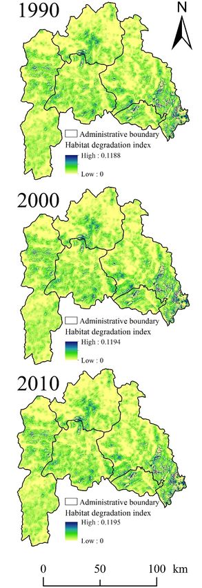
Sustainability 2018, 10, 3854                                                                      3 of 28

and landscape pattern. The changes ecological processes are of great significance to regional
maintenance of ecosystem service function and sustainable management. There were many models
developed to evaluate the function of ecosystems services, such as Multiscale Integrated Models
of Ecosystem Services (MIMES) [26], Artificial Intelligence for Ecosystem Services [27], Biodiversity
module in Integrated Valuation of Ecosystem Services and Tradeoffs model (InVEST) [28] and so on.
InVEST was developed as part of the Natural Capital Project [29], a partnership between Stanford
University, the University of Minnesota, The Nature Conservancy, and World Wildlife Fund in 2007,
whose aim is to provides a powerful tool for simultaneously quantifying and valuing multiple
ecosystem services generated by a landscape. InVEST can evaluate various service functions of
ecosystems such as biodiversity, soil conservation and carbon reserves, with advantages of less input
data, accurate output data and intuitive spatial visualization. InVEST thus was widely used by its
low application cost, high evaluation accuracy, and strong spatial analysis functions, which has been
successfully applied to comprehensive assessment of the ecosystems in different areas [30–32]. Patterns
in biodiversity are inherently spatial, therefore, which can be estimated by analyzing landscape maps
in conjunction with threats. The above researches all obtained good evaluation results, and the InVEST
model is proved scientific and effective.
      CA-Markov model and InVEST have achieved effective results in their respective fields,
less research has been done about the combination of two above models. By varying landscape and
evaluating the output from InVEST, we can provide useful information to managers and policy-makers
weighing the tradeoffs in ecosystem services, biodiversity conservation, and other landscape objectives.
The Three Gorges Project is the largest hydropower project in the world today, the construction of
which brings enormous benefits of flood control, electricity generation, shipping and water supply.
Likewise, it has a long-term but far-reaching impact on the ecology and environment of the reservoir
area and the whole basin. The ecological and environmental impact of the Three-Gorges Project has
been the focus of all worlds’ attention. As the special ecological functional zone, ecological security
status of TGRA concerns social and economic sustainable development of the whole Yangtze River
basin even the whole China. Owing to abundant in energy, resources and biodiversity, Hubei Section
of TGRA has become the essential area of natural environment construction. Many scholars have
studied the status of natural environment and the ecosystem health in this region, including ecological
environment sensitivity, ecosystem health condition, soil erosion sensitivity and so on [33,34].
      To better understand the impact of spatial and temporal dynamics in landscape pattern on
biodiversity in Hubei Section of TGRA, it is important to extract the landscape pattern and calculate
the habitat quality. This study therefore aimed to investigate and predict landscape pattern and habitat
quality by combining CA-Markov model and InVEST model, and explore biodiversity responses under
the influence of landscape pattern dynamics. Within the context of biodiversity decline, this study is
of practical implications for regional biodiversity conservation, natural environment protection and
economic sustainable development.

2. Materials and Methods

2.1. Study Area
      Hubei section of Three Gorges Reservoir Area (TGRA) is located in the middle reaches of the
Yangtze River, which lies at the head of the TGRA. The Hubei section of TGRA covers five parts
(Yiling districts, main urban areas of Yichang city, Zigui county, Xingshan county and Badong county),
extending from 110.06◦ to 111.65◦ E longitude and 31.06◦ to 31.56◦ N latitude (Figure 1). The total
area of this land is approximately 11,895 km2 , with a population of 1.48 million people. Mountains
and hills are the dominant terrain, with a summit that reaches 1000 to 2000 m. In addition to Yangtze
River, some headwater rivers and streams are located in northern parts of Badong county, southern
parts of Xingshan county and southeastern part of Yiling districts. This region has a typical subtropical
monsoon climate with an annual average precipitation from 1000 to 1400 mm. Sub-tropical evergreen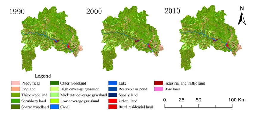
Sustainability 2018, 10, 3854 4 of 28
Sustainability 2018, 10, x FOR PEER REVIEW 4 of 28
tropical evergreen
broad-leaved forestbroad-leaved forest andforest
and warm coniferous warmare coniferous
the mainforest are thetypes.
vegetation main vegetation types.
The soil type The
mainly
soil type yellow
includes mainlybrown
includes yellow
soil, brown
rock soil, soil, soil,
yellow rock and
soil,purple
yellowsoil.
soil, and purple soil.
Figure 1. Geographic
Figure 1. Geographic location
location of
of study
study area.
area.
The
The study region is
study region is situated
situatedin inthe
thetransition
transitionzone
zonefrom
fromthethesecond
secondtotothethe third
third terrain
terrain ladder
ladder in
in
China, with abundant relic plants left over from quaternary glacier. As a rare plant gene bank in
China, with abundant relic plants left over from quaternary glacier. As a rare plant gene bank in
China,
China, there
there are
are many
many national
national forest
forest parks
parks and
and natural
natural reserves
reserves in in this
this region.
region. Abundant
Abundant water
water and
and
ore resources have made it one of the rarest eco-landscapes in China. Hence, the
ore resources have made it one of the rarest eco-landscapes in China. Hence, the natural environment natural environment
protection
protection is is of
of great
great importance
importance to to the
the construction
construction of of ecological
ecological civilization
civilization in in Hubei
Hubei province
province and
and
even in China. China Western Development, water conservancy and hydropower
even in China. China Western Development, water conservancy and hydropower projects, reservoir projects, reservoir
migration
migration and andother
otherfactors
factors have exerted
have exerteda profound
a profoundimpact on theon
impact ecological systemsystem
the ecological of TGRA, of leading
TGRA,
to the increased risk of ecological degradation for a long time. Construction of the
leading to the increased risk of ecological degradation for a long time. Construction of the 180-m-tall 180-m-tall dam was
officially
dam was started in started
officially 1994. After the Three
in 1994. After theGorges
ThreeReservoir impounding,
Gorges Reservoir the waterthe
impounding, level of dam
water levelhas
of
reached 135 m in 2003, 156 m in 2006, and 175 m in 2010. The construction of
dam has reached 135 m in 2003, 156 m in 2006, and 175 m in 2010. The construction of the Three the Three Gorges Dam may
have
Gorgesserious
Dam consequences
may have serious for plant and animal
consequences for species.
plant and Meanwhile, manyMeanwhile,
animal species. positive implementations
many positive
of policies and projects on vegetation protection promote the restoration
implementations of policies and projects on vegetation protection promote the restoration for ecosystem structure andfor
function of TGRA, such as Yangtze River protection forest engineering, natural
ecosystem structure and function of TGRA, such as Yangtze River protection forest engineering, forest protection project,
and returning
natural farmland toproject,
forest protection forest program.
and returning farmland to forest program.
2.2. Data Sources and Processing
2.2. Data Sources and Processing
2.2.1. Landscape Map
2.2.1. Landscape Map
To obtain the landscape pattern information of the study area, three sets of remote sensing images
To obtain
(respectively the landscape
obtained pattern
in1990, 2000 information
and 2010) need toof
bethe study area,
processed. three TM
Landsat-5 setsdata
of remote
with lowsensing
cloud
images (respectively obtained in1990, 2000 and 2010) need to be processed. Landsat-5
cover in summer time were selected as basic remote sensing sources. The Landsat-5 TM products with TM data with
low cloud cover in summer time were selected as basic remote sensing sources. The Landsat-5
a spatial resolution of 30m are available from the United States Geological Survey (USGS) [35] and have TM
products with a spatial resolution of 30m are available from the United States Geological
been calibrated and atmospherically corrected for gas, aerosol, and cirrus-cloud effects. Image mosaic Survey
(USGS)
and clip[35] and
were haveaccording
done been calibrated
to the and atmospherically
administrative corrected
boundaries of for gas,area,
study aerosol,
andand cirrus-cloud
remote sensing
effects. Image mosaic and clip were done according
images of the study area in1990, 2000 and 2010 were obtained.to the administrative boundaries of study area,
and remote sensing images
The landscape of the study
was classified on thearea in1990, 2000
reference and Use
of Land 2010Category
were obtained.
System of the Chinese
The landscape
Academy of Sciences.was classified
Table 1 shows onthe
thelandscape
reference category
of Land system
Use Category
for useSystem of the which
in our study, Chineseis
Academy of Sciences. Table 1 shows the landscape category system for use in our study,
divided into 6 classes of the first class and 25 classes of the second class. Based on three sets of TM which is
divided into 6 classes of the first class and 25 classes of the second class. Based on three sets of TM
images, the landscape pattern information was extracted by a combination method of supervised
images, the landscape pattern information was extracted by a combination method of supervised
classification and visual interpretation. To validate the accuracy of the landscape classification, 145 field
classification and visual interpretation. To validate the accuracy of the landscape classification, 145
field points were sampled in June 2010. The field accuracy of first-order classification reaches 90%,
and the second-order classification reaches 88%, which meet the research need.
Sustainability 2018, 10, 3854                                                                                 5 of 28

points were sampled in June 2010. The field accuracy of first-order classification reaches 90%, and the
second-order classification reaches 88%, which meet the research need.

                                           Table 1. Landscape category system.

      First Class                Second Class               First Class                 Second Class
                                   Paddy field                                     High coverage grassland
      Farmland
                                    Dry land                Grassland            Moderate coverage grassland
                                Thick woodland                                     Low coverage grassland
                                 Shrubbery land                                          Urban land
      Woodland
                                Sparse woodland         Construction land           Rural residential land
                                Other woodland                                    Industrial and traffic land
                                Canal                                                        Dene
                                 Lake                                                        Gobi
                           Reservoir or pond                                       Saline and alkaline land
        Waters
                        Permanent ice and snow             Unused land                    Marshland
                               Tideland                                                    Bare land
                              Shoaly land                                                  Bare rock
                                                                                            Other

2.2.2. Driving Factors
     According to the status of the study area, both natural and human factors were selected to analyze
driving forces for evolution of landscape pattern. Evaluation factors from two aspects of natural
environment conditions and location were chose as internal driving forces, including DEM, slope,
aspect, precipitation, temperature, distance to waters, distance to railway, distance to highway, distance
to national road, distance to provincial road, distance to county road, distance to urban land and
distance to residential land. As for external driving forces, population density and regional Gross
Domestic Product (GDP) were selected from aspects of social and economic development.
     DEM data was obtained from the ASTER Global Digital Elevation Model (ASTER GDEM) product,
which is developed by the U.S. National Aeronautics and Space Administration (NASA) and Japan’s
Ministry of Economy, Trade, and Industry (METI). The ASTER GDEM covers land surfaces between
83◦ N and 83◦ S, and referenced to the 1984 World Geodetic System (WGS84)/1996 Earth Gravitational
Model (EGM96) geoid. The product of ASTER GDEM Version 002 with spatial resolution of 30 m
are available from Land Processes Distributed Active Archive Center (LP DAAC) of United States
Geological Survey (USGS) [36]. The DEM data in 2010 of study region was processed and projected to
an Albers equal area conic projection. Based on DEM data, slope and aspect map were created and
extracted by using Slope and Aspect function of raster surface from 3D Analyst tools in ArcGIS 10.2.
     The precipitation and temperature data were downloaded from the Meteorological Data Sharing
Service System of China [37]. The annual average precipitation and air temperature data from
72 meteorological stations in 2010 that fully covered the entire region were selected. The annual
precipitation and temperature were interpolated from a point to a regional scale using a kriging
method with a spatial resolution of 30 m. Then, cross-validation was performed, and the interpolating
error were approximately 76.67 mm and 0.68 degree which meet the accuracy requirements.
     The spatial distribution of waters and construction land are all derived from the landscape map
of the study area. The buffer analysis and assignment were done by distance function in Idrisi 17,
and the buffer map of waters, traffic road at different level and town was drawn by setting 1.0 km
buffer radius.
     Night-time light data is a powerful tool to estimate socio-economic status as well as map gross
domestic product (GDP) distribution and urban expansion [38,39]. The DMSP-OLS NTL composite
has evolved into Version 4, containing global NTL time series 1992–2013. The composite for the year of
1992 and 2010 are available from the NOAA’s NGDC [40]. Due to lack of data before 1992, the year
composite data of 1992 was considered as night-time light data for the year of 1990. The stable light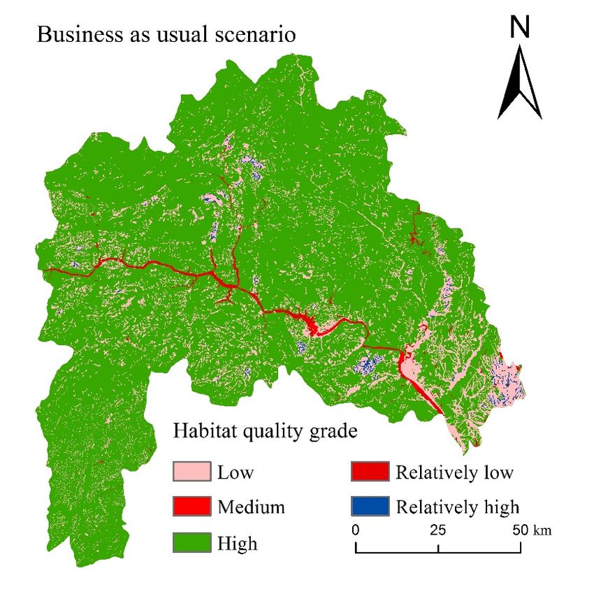
Sustainability 2018, 10, 3854                                                                               6 of 28

image, which has discarded ephemeral lights and background noise, from the composite was selected
to reflect GDP status. The stable light images in 1990 and 2010 of study region was processed and
projected to an Albers equal area conic projection.
     Furthermore, population data at the level of community in 1990 and 2010 were collected from the
fourth and sixth census of China respectively. Based on point data, Tyson polygons were constructed
and the population density of each polygons was calculated. Then, the regional population density
in 1990 and 2010 was obtained by interpolating points to a regional scale using an ordinary Kriging
method with a spatial resolution of 30 m.
     In the comprehensive evaluation of multiple factors, different factors often have different
dimensions and dimensional units. To eliminate the effect of dimension, dimensionless treatment
should be adopted before analysis. The data after dimensionless processing can accurately reflect the
information contained in the original data. According to the research needs and data characteristics,
equalization method in dimensionless treatment was used to reduce the loss of information in data
and preserve differences in variation degree among factors. The equalization method follows that:
                                                             xi
                                                     xi0 =                                                     (1)
                                                             xi

where, xi is the original value of each factor, and xi is the average value of all original value.

2.3. Methodology
     There were four main steps in conducting this research. Figure 2 shows the details for each
step. Firstly, the temporal and spatial variation characteristics of landscape pattern were analyzed by
calculating the transition matrix of Markov model. Secondly, the habit quality was evaluated by using
biodiversity module of InVEST model. Thirdly, the driving force for alterations in landscape pattern
was analyzed. Finally, Ca-Markov model together with InVEST model were used to simulate future
landscape pattern and Figure
                         habit2quality in 2020 under different scenarios.

          Figure 2. Flow chat for evolution and prediction of landscape pattern and biodiversity process.
                           Figure 4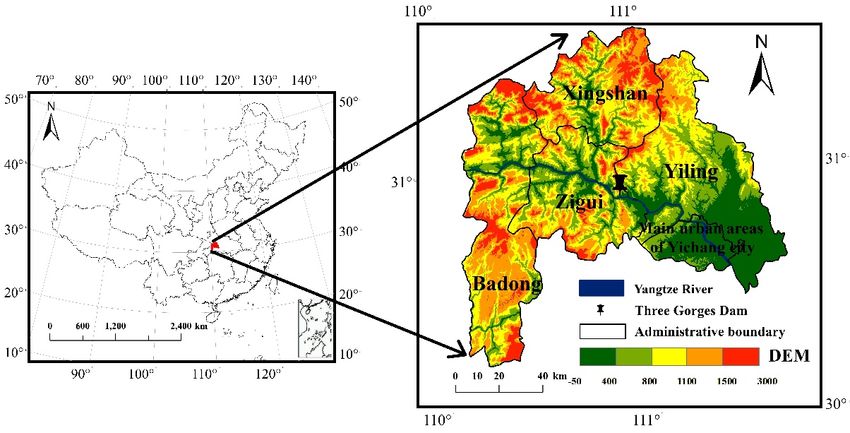
Sustainability 2018, 10, 3854 7 of 28
2.3.1. Markov Chain
Markov chain is the simplest of stochastic models which is a transition matrix [41], and has
been widely used for land cover change studies at various spatial scales [42]. In Markov model,
the initial probability and the transition probabilities between different states are calculated, and the
trend of landscape pattern changes over time is determined. Finally, the landscape pattern is predicted.
Please note that the transition between landscape types is often non-directional, which means that
the transition direction for the landscape types of current pixel allows for many possibilities in the
next moment [43]. The transition probability of each landscape type is different, and the size of
each possibilities are affected by many factors. The transition of landscape types is bi-directional,
which not only transit from the current types into other types, but also from other types to the current
types [44]. The types and quantity of landscape change constantly in the process of stochastic transition.
The transition process of landscape types accords with the conditions of Markov’s research, which is
difficult to describe accurately by mathematical methods [45,46]. The output of Markov model is the
probability of transition, Pij is between state i and j. In a landscape with multiple land covers or land
uses, the transition probability Pij would be the probability that a landscape type (pixels) i in time t0
changes to landscape type j in time t1. As the transitions are probabilities, it follows that:
···
P11 P1n
.. ..
P = . ... . (2)
Pn1 ... Pnn
where, n is number of landscape types, and Pij should meet two necessary conditions: 0 ≤ Pij ≤ 1;
∑nj=1 Pij = 1.
According to the principle of map algebra, the Markov transition matrix is established to
quantitatively analyze the direction and intensity of the transition between different landscape types
of second class. This transition matrix also can be used to predict the future landscape at time t2.
2.3.2. Habitat Quality
The biodiversity module in InVEST model maps the quality of habitat for a target conservation
objective [47]. Landscape maps are converted into habitat maps by defining what landscape counts
as habitat for various species [48]. Habitat quality is a function of the landscape type in a grid cell,
the landscape in surrounding grid cells, and the sensitivity of the habitat in the grid cell to the threats
posed by the surrounding landscape [49]. Landscape in surrounding grid cells can modify habitat
quality in a grid cell. Each landscape type is given a habitat suitability or quality score of 0 to 1 for
each particular measure of biodiversity with perfectly suitable habitat scored as 1 and non-habitat
scored as 0 [50].
Sources of degradation were considered as those human modified landscape types (e.g., urban,
agriculture, and roads) that cause edge effects [51,52]. Edge effects refer to changes in the biological and
physical conditions that occur at a patch boundary and within adjacent patches (e.g., facilitating entry of
predators, competitors, invasive species, toxic chemicals and other pollutants). The sensitivity of each
habitat type to degradation is general principles of landscape ecology and conservation biology [53,54],
and specific to each measure of biodiversity. The habitat quality was calculated combining landscape
types information and threats of biodiversity, and the equation is shown in formula (3):
!
Dxj 2
Q xj = Hj 1− (3)
Dxj 2 + k2
where the quality of habitat in grid cell x that is in landscape type j be given by Q xj . Hj represent the
habitat suitability. Q xj is equal to 0 if Hj = 0. Q xj increases in Hj and decreases in Dxj . The k constant
is the half-saturation constant and is set by the user. A grid cell’s degradation score is translated into
Sustainability 2018, 10, 3854                                                                                                     8 of 28

a habitat quality value using a half saturation function where the user determines the half-saturation
                                                                                                          Dxj2
value in InVEST model. The parameter k is equal to the D value where 1 −                                  2
                                                                                                         Dxj +k2
                                                                                                                    = 0.5.
    Dxj is the total threat level in grid cell x with landscape or habitat type j, and the equation is
shown in formula (4):                                     !
                                                    R   Yr                  R
                                          Dxj =   ∑∑             ωr /      ∑ ωr       ry irxy β x S jr                               (4)
                                                  r =1 y =1                r =1

where y indexes all grid cells on r’s raster map and Yr indicates the set of grid cells on r’s raster map.
S jr is the sensitivity of habitat type j to threat r where values closer to 1 indicate greater sensitivity.
Please note that each threat map can have a unique number of grid cells due to variation in raster
resolution If S jr = 0 then Dxj is not a function of threat r. Also note that threat weights are normalized
so that the sum across all threats weights equals 1.
       The impact of threat r that originates in grid cell y, ry , on habitat in grid cell x is given by irxy and
is represented by the following equations,

                                                                    d xy

                                            irxy = 1 −                                i f linear                                     (5)
                                                                 dr max

                                                   2.99
                                    irxy = exp −          d xy i f exponential                                                       (6)
                                                  dr max
where d xy is the linear distance between grid cells x and y and dr max is the maximum effective distance
of threat r’s reach across space. For example, if an exponential decline is selected and the maximum
impact distance of a threat is set at 1 km, the impact of the threat on a grid cell’s habitat will decline by
~50% when the grid cell is 200 m from r’s source. If irxy > 0 then grid cell x is in degradation source
ry ’s disturbance zone. ωr is the threat weight. β x indicates the level of accessibility in grid cell x where
1 indicates complete accessibility.
       Some input parameters in model were determined from the literatures [32,49] and 12 experts,
who are all in the field of regional ecological assessment and environmental simulation from the
key research and development project of typical vulnerable ecological restoration and protection in
China. The following parameters were input into the model, including landscape maps (three periods),
threats factor layers (including paddy field, dry land, urban land, rural resident land, industrial and
traffic land and bare land), index of threats and sensitivity (Table 2), weight of threat factor (Table 3),
sensitivity of landscape types to each threat, and accessibility to threats, and half-saturation constant.
The habitat quality maps were obtained after running the biodiversity module, and the grid resolution
was set to 30 m according to remote sensing data requirements. Habitat quality scores should be
interpreted as relative scores with higher scores indicating landscapes more favorable for the given
conservation objective. The score of landscape habitat quality cannot be interpreted as a prediction
of species persistence on the landscape or other direct measure of species conservation. The InVEST
habitat model does not convert habitat quality measures into monetary values.

                                Table 2. Landscape types and its sensitivity to each threat.

                                             Paddy           Dry            Urban           Rural        Industrial and      Bare
        Landscape Types           Habitat
                                             Fields          Land           Land        Resident Land     Traffic Land       Land
          Paddy field                0         0               1                 0               0                 0.5       0.4
           Dry land                  0         1               0                 0               0                 0.5       0.4
       Thick woodland                1         1               1                0.2             0.2                0.3       0.3
        Shrubbery land               1        0.5             0.5               0.2             0.2                0.2       0.1
       Sparse woodland               1        0.7             0.9               0.2             0.8                0.4       0.8
       Other woodland                1        0.5             0.5               0.2             0.2                 0         0
    High coverage grassland         0.5       0.8             0.8               0.4             0.7                0.4       0.4
      Moderate coverage
                                     1        0.5             0.5               0.2             0.2                0          0
           grassland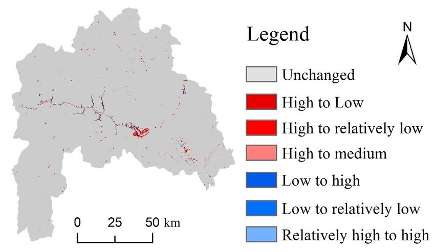
Sustainability 2018, 10, 3854                                                                                              9 of 28

                                                       Table 2. Cont.

                                             Paddy     Dry       Urban        Rural               Industrial and     Bare
        Landscape Types           Habitat
                                             Fields    Land      Land     Resident Land            Traffic Land      Land
     Low coverage grassland          1        0.8       0.8        0                0                  0.4            0.4
              Canal                  0        0.3       0.3       0.3              0.3                 0.8            0.2
               Lake                  1        0.5       0.4        0                0                  0.4            0.4
       Reservoir or pond             1         0         1        0.7              0.4                 0.4            0.6
          Shoaly land                1        0.8       0.8        0                0                  0.4            0.4
           Urban land                0         0         0         0                0                  0.8            0.7
      Rural residential land        0.6       0.2       0.2        0                0                   0             0.8
    Industrial and traffic land     0.7       0.2       0.2        0                0                   0             0.8
            Bare land               0.5       0.2       0.2        0                0                   0             0.8

                                             Table 3. Attributes of threat data.

                 Threat                   Maximum Effective Distance (km)                Weight               DECAY
           Paddy fields                                  0.5                              0.5                Exponential
             Dry land                                    0.5                              0.5                Exponential
            Urban land                                    3                               0.7                Exponential
       Rural residential land                             2                               0.7                Exponential
     Industrial and traffic land                          8                                1                   Linear
             Bare land                                   10                               0.3                Exponential

2.3.3. Logistic Regression Model
     Logistic Regression (LR) model is a nonlinear model, forming a multivariate regression relation
between a dependent variable and a set of independent variables [55,56]. The principle of LR rests
on the analysis of a problem, in which a result measured with dichotomous variables such as 0 and
1 or true and false, is determined from one or more independent factors [57]. The goal of LR is to
find the best fitting (yet reasonable) model to describe the relationship between a dependent variable
(the presence or absence of event) and a set of independent variables [58,59]. Compared with linear
regression analysis models, the advantage of LR is that the variables may be either continuous or
discrete, the value of variable can be any value in the real number range, and they do not necessarily
follow normal distributions. Maximum likelihood estimation is used in the algorithm of LR model after
transforming the dependent variable into a logit variable [55,60]. Logistic regression has been widely
applied for driving force analysis by many researchers [58–63], which can generate the regression
relation with dichotomous variables such as 0 and 1 or true and false [64]. The equation of LR
model follows (7):

                                 Pi
                      Y = lg            = logit( Pi ) = ∝ + β 1 X1 + β 2 X2 + · · · + β n Xn       (7)
                               1 − Pi

                                                                 ey
                                                       Pi =                                                                   (8)
                                                               1 + ey
where, Pi is the probability that a certain landscape type i may appear or disappear in each grid.
Function Y is represented as logit( Pi ), i.e., the log (to base e) of the odds or likelihood ratio that the
dependent variable. Xn denotes each influencing factor. ∝ represents the constant term. β 1 , β 2 , · · · , β n
are the partial regression coefficient of LR model, representing the impact of the independent variable
Xn on Y. When the coefficient is positive and statistically significant, which means that the event
of Y event is more likely to occur as the value of corresponding independent variables increases
under the control of other independent variables. When the coefficient is negative and statistically
significant, which means that the odds of the event Y occurring decreases as the value of corresponding
independent variables increases under the control of other independent variables. A coefficient of 0
does not change the odds one way or another.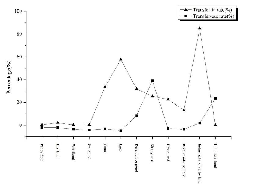
Sustainability 2018, 10, 3854                                                                        10 of 28

      In this study, LR establishes a functional relationship between the binary coded landscape
locations (presence or absence of a landscape) and different factors that are recognized as playing a role
in landscape development. For each landscape type, when the landscape type is changed, its value is
set as Y = 1; otherwise, Y = 0. LR generates the model statistics and coefficients of a formula useful
to describe the relationship between the binary coded landscape locations (presence or absence of
a landscape) and different factors. Relative Operating Characteristics (ROC) is usually used to test the
regression effect [65].
      LR model estimates the probability of a certain event occurring, therefore, selecting influencing
factors that have a significant impact on the landscape pattern, and determining the quantitative
relationship between them. According to the status of the study area, both natural and human factors
were selected to construct the index system of driving forces for landscape evolution, and each factor
was spatialized. Before the analyzing work of LR model, it is necessary to normalize the data of
different measuring scales. The results should be interpreted with caution if the data fail to normalized
in a manner LR model needs. In the application for exploring influencing factors on landscape
variation, the common solution is to create layers of binary values for each class of an independent
parameter [59,66,67]. Here, we used binary landscape data (when the landscape type is changed, its
value is 1; otherwise, 0.) from all over the area. Then, the driving mechanism of landscape evolution
from 1990 to 2010 can be explored by using LR model.

2.3.4. CA-Markov Model
     CA-Markov model consists of Markov chain and Cellular Automata (CA) model. As a method
of studying nonlinear science, CA model is a spatially dynamic model, whose time, space and state
are discrete. CA model consists of four parts, including cellular and its state, cellular space, cellular
neighborhood and transition rules. In cellular space, every cell has its limited and particular state,
and will be update according to the defined local rules. The interaction of these local rules forms
a dynamic evolution system. In a CA model, the transition of a cell from one landscape to another
depends on the state of the neighborhood cells [68]. A cell will have a higher probability to transit
to land-use type ‘A’ than to a land-use type ‘B’ if the cell is in closer proximity to land-use type ‘A’.
Thus, the CA model not only uses the information of the previous state of a landscape type as done by
a Markov model but also uses the state of neighborhood cells for its transition rules.
     CA model has been widely used for land use and land cover (LULC) change analysis, which can
be expressed by the following formula:

                                           S ( t +1) = f S ( t ) , N                                     (9)

where, S is the set of finite and discrete cellular states, t and t + 1 represent different moment in time,
N is cellular neighborhood, and f is the cellular transition rules in local space.
     CA model adds spatial character to a Markov model, thus combining CA-Markov model.
In CA-Markov model, each landscape pixel is a cellular, and the landscape type of each cellular
refers to a cellular state. With the support of GIS software, the transition of cellular state is determined
by calculating the transition area matrix and conditional transition probability maps, and the change
of landscape pattern is simulated [23]. CA-Markov module of IDRISI 17 was used to predict future
landscape. The specific implementation process is as follows:
     In the first step, a Markov model is run using the landscape maps of different period to predict
for future. In doing so, the CA Markov model makes the assumption that the driving factors affecting
change in all time periods are same. The outputs of this step are a transition area matrix, a transition
probability matrix and a series of transition probability maps (probability of each pixel to each
landscape types).
     In the second step, CA analysis is run using the landscape maps and outputs from the Markov
module, i.e., transition area matrix, transition probability maps and contiguity. The combined cellular
Sustainability 2018, 10, 3854 11 of 28
automata and Markov chain method of the CA Markov module adds an element of spatial contiguity as
well as knowledge of the likely spatial distribution of transitions to Markov chain analysis. The inherent
suitability of each pixel and the restriction factors for each landscape types are established. The inherent
suitability of each pixel is obtained by using the transition probability maps in an iterative process of
CA Markov module. It is considered that within a certain threshold value, the suitability is the highest,
which is set for 1. When exceeding the threshold, the Sigmoid function decreases with the distance
until the extremely unsuitable distance is reached, and the adaptability is set for 0. After exceeding
this distance, the suitability will not change. Next, an Analytic Hierarchy Process (AHP) method is
used to weight sum the suitability layers the results of LR analysis. Then, OWA aggregation is done by
selecting Location 4. In addition, the restriction factors obtained by LR analysis also were selected to
put in model.
In the third step, the start time and the number of CA cycles were determined. One year represents
one iteration, the iteration is taken as 10. For our present study, the time period of 1990 and 2000 should
be used as reference map for validating the corresponding dates predicted maps of 2010, because the
data were not used to build the respective models. If the predicted 2010 map is similar to reference
2010 map, we considered that the model performed well.
In the final step, validation was done simply by cross tabulating the predicted and observed
landscape map of respective years. In present study, the predicted landscape map of 2010 was used to
compare with reference 2010 map. The Kappa index was used to test the prediction accuracy of model,
which can be expressed by the following formula:
Kappa = (P0 − Pc )/(P0 + Pc ) (10)
where P0 is the correct ratio of simulation, Pc is the correct ratio of random simulation, and Pp is the
correct ratio of ideal classification.
3. Results
3.1. Spatial Landscape Pattern Analysis
Woodland, farmland and grassland are the main landscape types in the study area, accounting for
95% of the total area, of which 75% is woodland (Figure 3). From 1990 to 2010, the landscape pattern
of the study area has changed slightly (Figure 4). Among the landscape types, woodland, waters
and construction land had the greatest change in proportion. The area of woodland, farmland and
grassland has been decreasing gradually, and the area of waters and construction land increased in
the past two decades. The area of unused land slightly declined. The area of woodland, farmland
and grassland in 1990 were 9631.88 km2 , 1598.50 km2 and 815.38 km2 . By 2010, the area of above
landscape types was 9539.11 km2 , 1579.64 km2 and 813.85 km2 respectively. The area of waters and
construction land in 1990 were 131.02 km2 and 67.71 km2 , and the area of above landscape types was
190.50 km2 and 121.51 km2 in 2010. These landscape variations fit the facts of the Three Gorges Dam
construction, impoundment of the Three Gorges Reservoir, immigration and expansion of construction
land in study area.
Figure 5 exhibits the landscape transition map from 1990 to 2010 by overlaying landscape maps
of before and after periods. The landscape transition matrix was statistically sorted. The results
showed that 98.62% of the landscape types did not change within 20 years, and only about 1.38% of the
landscape types changed (Table 4). The most varied landscape types were woodland, farmland, waters
and construction land. The land occupancy of Three Gorge Dam construction and the impoundment
of TGR could be the reason for the decreasing area of woodland and farmland located with the average
elevation of 140 m. The increasing area of waters and construction land could be explained by the
impoundment of TGR, migration and resettlement, and urbanization.and grassland in 1990 were 9631.88 km , 1598.50 km and 815.38 km . By 2010, the area of above
landscape types was 9539.11 km2, 1579.64 km2 and 813.85 km2 respectively. The area of waters and
construction land in 1990 were 131.02 km2 and 67.71 km2, and the area of above landscape types was
190.50 km2 and 121.51 km2 in 2010. These landscape variations fit the facts of the Three Gorges Dam
construction, impoundment of the Three Gorges Reservoir, immigration and expansion of
Sustainability 2018, 10, 3854 12 of 28
construction land in study area.
Figure 4 Figure 3. Spatial distribution maps of landscape in 1990, 2000, 2010.
Figure 3. Spatial distribution maps of landscape in 1990, 2000, 2010.
Figure 5
Figure 4. Landscape area of first class in 1990, 2000 and 2010.
1
Figure 5. Spatial variation map of landscape pattern between 1990 and 2010.
Figure 6Sustainability 2018, 10, 3854 13 of 28
Figure 6 illustrates the transfer in and out rate of landscape types. From 1990 to 2010, shoaly
land and unused land had relatively high transfer-out rate, with a decreasing ratio of 41.86% and
27.05% respectively. Most of shoaly land mainly transferred into canal and reservoir or pond. Unused
land mainly transferred into urban land, industrial and traffic land. Waters (canal, lake, reservoir or
pond) and industrial and traffic land had relatively high transfer-in rate. Industrial and traffic land
has highest transfer-in rate. The area of industrial and traffic land in 2010 was six times bigger than in
1990, and they were mainly transferred from woodland and farmland. Lake has the second-highest
transfer-in rate with an increasing ratio of 136.36%, mainly transferring from woodland.
In the whole study area, waters and construction land have been the most dramatic changed
landscape types. These variations mainly concentrated in main urban areas of Yichang city, extending
downstream along the Yangtze River. Some of the variation located in Badong County. The expansion
of waters was distributed around Three Gorges dam site in Zigui County and along the main and
tributary banks of5the Yangtze River. The strong increasing trend of construction land could be
Figure
explained by the continuous improvement of settlement scale, the demand for supporting and
improving facilities after three periods of immigration of the pilot project.
Table 4. Statistics information of main landscape changing types from 1990 to 2010 (km2 , %)
Changed Type Area Percentage
Unchanged 12,067.19 98.62
Woodland to canals 41.52 0.34
Woodland to industrial and traffic land 26.21 0.22
Woodland to reservoir or pond 8.23 0.07
Woodland to urban land 6.84 0.06
Paddy fields to canal 3.82 0.03
Paddy field to industrial and traffic land 3.77 0.03
Paddy fields to urban land 3.43 0.03
Dry land to urban land 3.31 0.03
Dry land to industrial and traffic land 3.28 0.03
Dry land to canals 2.95 0.02
Woodland to rural residential land 2.90 0.02
Paddy fields to reservoir or pond 2.51 0.02
Paddy fields to rural residential land 2.32 0.02
Figure 6
Figure 6. Transfer rate of landscape types between 1990 and 2010.
2Sustainability 2018, 10, 3854 14 of 28
3.2. Spatial and Temporal Variation of Biodiversity
3.2.1. Analysis of Habitat Degradation
The value of habitat degradation index ranging from 0 to 1 represents the relative habitat
degradation level of the current landscape, where 1 denotes high degradation and 0 denotes low
degradation. Figure 7 shows the spatial distribution map of habitat degradation. The maximum
value of habitat degradation index were 0.1188, 0.1194 and 0.1195 respectively, showing a gradually
increasingSustainability
trend from 2018,1990 to PEER
10, x FOR 2010. In terms of spatial pattern, the areas with higher habitat
REVIEW degradation
14 of 28
index were mainly distributed in main urban areas of Yichang city, southeastern parts of Yiling districts
degradation index were mainly distributed in main urban areas of Yichang city, southeastern parts
and south-central parts of Xingshan county, and the corresponding landscape types were urban land,
of Yiling districts and south-central parts of Xingshan county, and the corresponding landscape types
rural residential land
were urban land, and canal.
rural The areas
residential with
land and relatively
canal. The areaslow
withhabitat
relativelydegradation index were mainly
low habitat degradation
distributed in the central and southwest of study area, such as Zigui county and Badong county,
index were mainly distributed in the central and southwest of study area, such as Zigui county and and the
Badong county, and the corresponding landscape type was woodland. Overall,
corresponding landscape type was woodland. Overall, the TGR area (Hubei section) developed rapidly the TGR area (Hubei
section) developed rapidly from 1990 to 2010, causing a causing a continuously increasing trend of
from 1990habitat
to 2010, causing a causing a continuously increasing trend of habitat degradation.
degradation.
Figure 7.Figure 7. Spatial
Spatial distribution
distribution patternof
pattern of habitat
habitatdegradation indexindex
degradation in 1990,in2000,
1990,2010.
2000, 2010.Sustainability 2018, 10, 3854 15 of 28
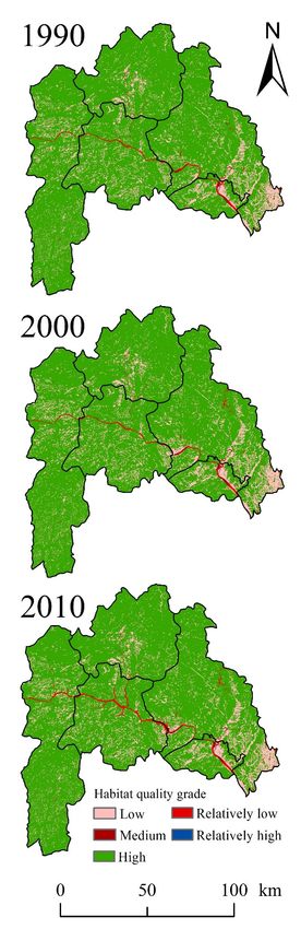
3.2.2. Analysis of Habitat Quality
Higher values indicate better habitat quality vis-a-vis the distribution of habitat quality across the
rest of the landscape. To facilitate the observation of changes in habitat quality, the division method
of natural breaks was adopted to assign grades according to the output values of habitat quality.
The habitat quality was divided into five grades, they are low, relatively low, medium, relatively
high, and high, and these grades are on behalf of poor habitat quality, relatively poor habitat quality,
medium habitat quality, relatively high habitat quality, and high habitat quality respectively (Table 5).
Table 5. Classification value of habitat quality in study area
Grade Value Range Description
Low 0~0.1 Poor habitat quality
Relatively low 0.1~0.6 Relatively poor habitat quality
Medium 0.6~0.8 Medium habitat quality
Relatively high 0.8~0.9 Relatively high habitat quality
High 0.9~1 High habitat quality
Based on divisions, the spatial distribution map of habitat quality grade in three phases was
obtained (Figure 8), and the variations of habitat quality were statistically analyzed (Table 6). Overall,
woodland, farmland and grassland occupied for 95% of the total area, thus the habitat quality of whole
area was at a relatively high grade. The areas with high habitat quality grade was mainly distributed
in Badang, Zigui and Xingshan county where the coverage of woodland. The areas with low habitat
quality grade was mainly distributed in main urban areas of Yichang city, southeastern parts of Yiling
districts, southern parts of Xingshan county and shoaly areas along the banks of the Yangtze River,
where the corresponding landscape types are construction land and canals with higher elevation.
The overall habitat quality score declined slightly from 1990 to 2010. Habitat quality achieved
a score of 0.8653 in 1990, 0.8259 in 2000 and 0.8155 in 2010. Most of areas was in a relatively high
grade of habitat quality, the overall score of habitat quality decreased over the past twenty years.
The magnitude of the declines for overall habitat quality was likely to be slight, but obvious in some
local areas. The area of landscape with high habitat quality grade decreased obviously. The area of
landscape with low and relatively low habitat quality grade increased. In 1990, the areas with high
grade of habitat quality occupied for 84.78% of the total area, and accounted for 84.02% in 2010 with
a decline area of 0.76%. The area of low and relatively low habitat quality grade increased by 0.3% and
0.44% respectively.
The overall habitat quality continues to decrease and the urbanization process continues to
develop combining with the analysis of the habitat degradation. From 1990 to 2010, the overall
fluctuation of habitat quality was relatively small, and the variation areas mainly were distributed
in urban areas, canal areas with higher elevation and areas along the banks of the Yangtze River.
In general, the fluctuation of habitat quality tended to be stable as a whole.
Based on habitat quality maps of 1990 and 2010, spatial changes of habitat quality were obtained in
the past two decades (Figure 9). The landscape transition showed a decreasing trend of habitat quality
grade from high to low and relatively low grade in areas of study region. The changes of habitat quality
grade from high to low grade were that large areas of woodland and grassland have been developed
for residential land, industrial and traffic land. The changes of habitat quality grade from high to
relatively low grade were the transitions from woodland and grassland to canals. The construction
of the Three Gorges Dam, impoundment in the TGR area and environmental migration contributed
the increasing area of construction land and waters, decreasing area of woodland and grassland,
and a decline of habitat quality as a whole.Sustainability
Sustainability 2018,
2018, 10,
10, x3854
FOR PEER REVIEW 16
16of
of28
28
Figure 8. Spatial distribution pattern of habitat quality in 1990, 2000, 2010.
Figure 8. Spatial distribution pattern of habitat quality in 1990, 2000, 2010.Sustainability 2018, 10, 3854 17 of 28
Sustainability 2018, 10, x FOR PEER REVIEW 17 of 28
Figure 9. Spatial variation map of habitat quality between 1990 and 2010.
Figure 9. Spatial variation map of habitat quality between 1990 and 2010.
Table 6. Area and percentage of habitat quality at all grades (km2 , %)
Table 6. Area and percentage of habitat quality at all grades (km2, %)
1990 2000 2010 1990 to 2010
Grade
1990
Area Percentage 2000 Percentage
Area Area 2010
Percentage Area 1990 to 2010
Percentage
Grade
Low Area Percentage
1664.66 13.60 Area
1707.71 Percentage
13.95 Area
1701.48 Percentage
13.90 Area
36.81 Percentage
0.30
Low Relatively1664.66
low 100.28 13.60 0.82 1707.71 99.53 13.95
0.81 1701.48
153.90 13.90
1.26 36.81
53.62 0.44 0.30
Medium
Relatively 30.18 0.25 32.14 0.26 36.27 0.30 6.08 0.05
100.28 68.45 0.82 0.56 99.5367.83
Relatively high 0.810.55 153.90
65.39 1.26
0.53 53.62
−3.06 −0.030.44
low High 10,379.36 84.78 10,337.74 84.42 10,287.91 84.02 −91.45 −0.76
Medium 30.18 0.25 32.14 0.26 36.27 0.30 6.08 0.05
Relatively
3.3. Driving 68.45
Force for Spatial
0.56Variation 67.83
of Landscape 0.55
Pattern 65.39 0.53 −3.06 −0.03
high
High With 10,379.36
the construction 84.78of Dam, impoundment
10,337.74 84.42 and 10,287.91
reservoir resettlement
84.02 in the TGR −0.76
−91.45 area,
the landscape pattern has been changed, leading to the decline of habitat quality. According to
statistics
3.3. of landscape
Driving pattern,
Force for Spatial the most
Variation varied landscape
of Landscape Pattern types were woodland, farmland, waters and
construction land. Hence, both natural factors and human factors were selected to explore the driving
With the construction of Dam, impoundment and reservoir resettlement in the TGR area, the
mechanism of spatial variation of landscape pattern. To investigate the most dominant influencing
landscape pattern has been changed, leading to the decline of habitat quality. According to statistics
factors, the following 15 factors are listed, including Night-time light (X1 ), population density (X2 ),
of landscape pattern, the most varied landscape types were woodland, farmland, waters and
DEM (X3 ), slope (X4 ), aspect (X5 ), precipitation (X6 ), temperature (X7 ), distance to waters (X8 ), distance
construction land. Hence, both natural factors and human factors were selected to explore the driving
to railway (X ), distance to highway (X10 ), distance to national road (X11 ), distance to provincial road
mechanism of9 spatial variation of landscape pattern. To investigate the most dominant influencing
(X12 ), distance to county road (X13 ), distance to urban land (X14 ), and distance to rural residential land
factors, the following 15 factors are listed, including Night-time light (X1), population density (X2),
(X15 ). Table 7 shows the results of LR analysis.
DEM (X3), slope (X4), aspect (X5), precipitation (X6), temperature (X7), distance to waters (X8), distance
to railway (X9), distance to highway (X10), distance to national road (X11), distance to provincial road
(X12), distance to county road (X13), distance to urban land (X14), and distance to rural residential land
(X15). Table 7 shows the results of LR analysis.Sustainability 2018, 10, 3854 18 of 28
Table 7. Results of Logistic regression analysis.
Independent Paddy Reservoir Shoaly Urban Rural Industrial and Bare
Dry Land Woodland Grassland Canal Lake
Parameter Field or Pond Land Land Residential Land Traffic Land Land
Intercept −4.30 −2.62 −2.34 −0.11 17.70 −161.50 1.29 −18.74 −378.72 −37.42 −28.93 −1136.34
X1 −0.79 0.44 0.40 84.61 543.06 2.21 −0.64 2.15 7.13 827.33 0.00 392.10
X2 −0.49 −0.40 −0.84 −0.38 −0.05 6.94 1.23 −0.38 −1.35 1.52 −2.09 4.08
X3 −58.21 −4.04 −32.79 4.45 −369 −368.32 102.37 202.56 124.07 9.55 −74.06 478.59
X4 71.12 7.93 48.93 3.81 428.69 480.34 −130.03 −193.84 −11.88 316.47 71.66 −705.36
X5 2.60 1.08 −5.16 −10.89 −17.26 −74.72 23.38 −8.73 −23.62 −9.02 21.00 −24.43
X6 1.80 −13.27 −12.43 −40.05 −300 1757.60 87.07 −161.30 −1079.92 483.07 298.85 16,293.71
X7 −1.70 16.32 15.94 48.65 363.17 −2082 −87.57 159.51 467,520 −587.76 −362.09 −19725
X8 0.10 0.03 −0.08 0.00 −0.73 7.65 −0.59 −0.15 −1.05 0.81 0.33 −5.64
X9 0.00 −0.01 0.04 −0.02 0.13 0.00 −0.12 0.10 −0.06 0.37 0.02 −12.95
X10 0.07 0.02 0.07 0.13 0.35 −1.82 0.06 −0.02 −1.04 −0.39 −0.79 −9.33
X11 0.04 0.02 0.12 0.00 0.30 0.05 0.11 0.06 −0.10 0.36 0.34 12.06
X12 0.01 0.02 −0.12 −0.03 0.33 4.41 0.20 −0.44 2.00 1.07 −0.25 43.52
X13 −0.44 −0.18 −0.37 −0.39 0.35 8.53 −0.44 0.02 0.28 1.21 −2.23 23.70
X14 −0.07 −0.07 −0.14 −0.08 −0.51 −7.18 0.22 0.03 −192.14 −0.97 −0.08 −105.56
X15 0.21 −0.06 0.04 −0.12 0.53 −2.62 0.55 0.06 −1.40 −349.51 0.33 9.22
ROC 0.94 0.83 0.92 0.86 0.99 0.85 0.95 0.98 0.90 0.88 0.98 0.87You can also read