Field Calibration of TDR to Assess the Soil Moisture of Drained Peatland Surface Layers - MDPI
←
→
Page content transcription
If your browser does not render page correctly, please read the page content below
water
Article
Field Calibration of TDR to Assess the Soil
Moisture of Drained Peatland Surface Layers
Tomasz Gnatowski 1, * , Jan Szatyłowicz 1 , Bogumiła Pawluśkiewicz 1 , Ryszard Oleszczuk 1 ,
Maria Janicka 2 , Ewa Papierowska 3 and Daniel Szejba 1
 1   Department of Environmental Improvement, Faculty of Civil and Environmental Engineering, Warsaw
     University of Life Sciences—SGGW, Nowoursynowska159, 02-776 Warsaw, Poland;
     jan_szatylowicz@sggw.pl (J.S.); bogumila_pawluskiewicz@sggw.pl (B.P.); ryszard_oleszczuk@sggw.pl (R.O.);
     daniel_szejba@sggw.pl (D.S.)
 2   Department of Agronomy, Faculty of Agriculture and Biology, Warsaw University of Life Sciences—SGGW,
     Nowoursynowska159, 02-776 Warsaw, Poland; maria_janicka@sggw.pl
 3   Laboratory Water Center, Faculty of Civil and Environmental Engineering, Warsaw University of Life
     Sciences—SGGW, Nowoursynowska159, 02-776 Warsaw, Poland; ewa_papierowska@sggw.pl
 *   Correspondence: tomasz_gnatowski@sggw.pl; Tel.: +48-22-593-53-63

 Received: 8 October 2018; Accepted: 29 November 2018; Published: 13 December 2018

 Abstract: The proper monitoring of soil moisture content is important to understand water-related
 processes in peatland ecosystems. Time domain reflectometry (TDR) is a popular method used for soil
 moisture content measurements, the applicability of which is still challenging in field studies due to
 requirements regarding the calibration curve which converts the dielectric constant into the soil
 moisture content. The main objective of this study was to develop a general calibration equation for
 the TDR method based on simultaneous field measurements of the dielectric constant and gravimetric
 water content in the surface layers of degraded peatlands. Data were collected during field campaigns
 conducted temporarily between the years 2006 and 2016 at the drained peatland Kuwasy located in
 the north-east area of Poland. Based on the data analysis, a two-slopes linear calibration equation was
 developed as a general broken-line model (GBLM). A site-specific calibration model (SSM-D) for the
 TDR method was obtained in the form of a two-slopes equation describing the relationship between
 the soil moisture content and the dielectric constant and introducing the bioindices as covariates
 relating to plant species biodiversity and the state of the habitats. The root mean squared error for
 the GBLM and SSM-D models were equal, respectively, at 0.04 and 0.035 cm3 cm−3 .

 Keywords: degraded peat soils; dielectric constant; TDR calibration curve; broken-line model;
 bioindices of habitats

1. Introduction
     Accurate determination of soil moisture is important for various hydrological, agricultural and
environmental applications. In hydrology, soil moisture content plays a major role in the water cycle
by controlling hydrological fluxes, such as infiltration, runoff and groundwater recharge [1]. In climate
studies, soil moisture governs the energy flux exchange between the land surface and the atmosphere
through its impact on evapotranspiration [2]. Determination of the soil moisture content is very
important for hydrological studies in peatland soils, the actual condition and preservation of which
depends on water-related processes [3–5]. Peatland soils occupy about 400 million hectares, which
is about 3% of the world’s land [6]. Most of these soils are located in the northern part of the globe,
including large areas of North America, Europe and Russia. It is estimated that peat soils contain
about one-third of global soil organic carbon stock [7]. The last GIS-based estimation of peatland areas
in Europe shows that this type of ecosystems occupies approximately 593,727 km2 and 46% of this area

Water 2018, 10, 1842; doi:10.3390/w10121842                                      www.mdpi.com/journal/water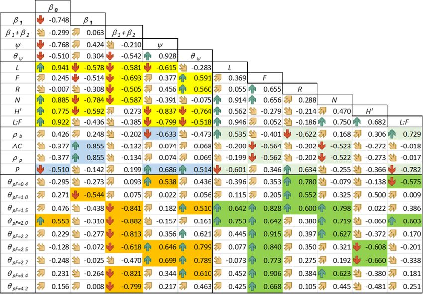
Water 2018, 10, 1842                                                                                2 of 22

is classified as peatland where the peat forming process was stopped [8]. Stopping the forming process
was associated with artificial land drainage in response to agricultural, forestry and horticultural
demands [9]. The great majority of drained peatland is used as meadow and pasture, and only a
limited percent as arable land [10]. Drainage of peat soils leads to the formation of a new organic soil
material in the surface layers known as muck (moorsh), which has a granular structure where the
original plant remains are not recognizable and contains more mineral matter than peat [11].
      Soils contain twice as much organic carbon than the amount of C in the atmosphere [12], therefore
any changes in the terrestrial pool are usually associated with the impact of global warming [13,14].
The importance of peatlands in global warming relates to the fact that 14% to 20% of these areas
globally are currently used for agriculture, mainly as meadows or pastures, and oxidized soils of these
ecosystems are a source of carbon, which has an influence on the global increase of CO2 emissions [15].
A literature review shows that there are three major factors used to quantify the amount of CO2
emission from drained peat soils, i.e., soil temperature [16–18], soil moisture content status [17,19,20]
and water table depth [21]. The increase of soil temperature and optimal soil moisture status create
favorable conditions for the increase of CO2 efflux. Soil moisture content is one of the main hydrological
factors to be assessed in the calibration and validation of activities in global soil moisture products
(spaceborne), as well as in order to increase the understanding of water, energy and carbon flux
exchanges at the active surface on a local scale [22].
      Over the last four decades, the most popular in situ soil moisture measuring technique was
based on measurements of the dielectric properties of the medium in time domain. This method is
named Time Domain Reflectometry (TDR) and its first application in soil science was reported in
1980 [23]. The theory behind this measurement technique is based on travel time analysis of the short
electromagnetic step pulse which formed an electrical field along a waveguide (e.g., two parallel
rods of a given length) surrounded by the soil [24]. The time required to travel the length of the
waveguide (there and back) is recorded and used to calculate the dielectric constant (Ka ) of the
medium [25]. The attractiveness of the TDR method results from the simple non-destructive and
quick measurement of the dielectric constant which can be transformed using the calibration curve to
the volumetric soil moisture content. However, many TDR probes on the market are often not
properly tested for the high dielectric permittivity values of peat soils and that the algorithms for
the TDR waveform analysis might fail in that range [26]. The relationship between the measured
Ka and moisture content can be derived either by using the dielectric mixing model [27,28] or by
empirical equations [25]. In peat soils, in most cases, the calibration curves are empirical equations
obtained by fitting a mathematical model of the measured dielectric constant to the gravimetrically
measured soil moisture content data. The majority of calibration equations for peat soils are third-order
polynomials with respect to the raw measured dielectric constant [22,23,29–32] or its transformed form
as a square root [33]. The polynomial calibration equations are very flexible and more efficient than
the manufacturer default relationships (determined by developers of the TDR measurement systems)
but they are appropriate as a site- or soil-specific equations which enables improved accuracy of soil
moisture content estimation [34]. A more general calibration equation for the organic materials can also
be expressed in the form of a nonlinear relationship between the soil moisture content and the dielectric
constant [22,35,36]. Another popular group of empirical equations constitutes the linear relationship
between the soil moisture content and the square root of the dielectric constant. Malicki et al. [37]
developed an empirical model which incorporates soil bulk density as second covariate, in addition
to the Ka0.5 , thereby improving the moisture content predictions for a broad range of soils, also
including organic soils. Oleszczuk et al. [38], using a similar data analysis technique, obtained a
general empirical model describing soil moisture content as a function of the dielectric constant, bulk
density and ash content for different top organic soil layers from the Biebrza River Valley. However,
this type of calibration procedure, apart from the dielectric constant measurements, requires extra
knowledge regarding other soil properties in order to predict its moisture content status. Despite
the large number of calibration equations for determination of the soil moisture content using TDR,
Water 2018, 10, 1842 3 of 22
they were developed mostly under laboratory conditions and their use is limited to specific sites or
dedicated soils.
Peat soils are characterized by soil volume changes due to soil moisture content changes. Peat soil
shrinks during drying and its bulk density increases while wetting, causing soil swelling and a decrease
in bulk density [36,39–42]. In the majority of laboratory calibrations using TDR, bulk density changes
are not considered as a factor influencing the dielectric constant.
Interdependence of peat properties and vegetation cover is often observed in peatlands [43].
The linkage between the physical and chemical properties of soil and the state of plant cover is often
described using diversity indices representing plant species [44] or using more complex environmental
indicators [45]. Biodiversity is a useful metric for quantifying the composition and abundances of the
plant species [46] providing information about community structure and it may also be used as an
indicator of the ecosystem’s health [47]. In Europe, the Shannon–Wiener index (H’) is a commonly
used bioindicator for ecological assessment of the quality of ecosystems [48]. According to its value,
the ecosystem’s status can be classed from “Bad” (H’ ≤1) to “High” (H’ >4). In between there are three
classes of ecosystem quality: “Poor” (1 < H’ ≤ 2), “Moderate” (2 < H’ ≤ 3) and “Good” (3 < H’ ≤ 4).
The species composition of grassland is considered a good indicator of habitat properties which are
frequently quantified using species indicator values [49]. Ellenberg indicator values (EIV) [45] are
the most commonly used ecological indicators in Central Europe because they summarize complex
environmental factors including: Groundwater level, soil moisture content, precipitation, humidity,
etc. in one figure and they are calculated on the basis of complete species composition of plant
communities [50]. The system of indicators, as compiled by [45], considers vascular plant species
with respect to: Light intensity (L), mean annual air temperature (T), continentality (K), substrate
moisture (F), substrate reaction (R), substrate nutrient availability (N) and salt content of the substrate
(S). Six of these indicators have a nine-point scale and 12 levels have been established for the F value.
The present definition of the EIV system and the re-interpretation of the L indicator were presented in
the study by [51]. Despite the ordinal character of the EIV indicators [50], their average estimators of
a vegetation record provide helpful environmental site information, which can substitute costly and
time-consuming measurements [52–54].
Taking into account the importance and range of occurrence of drained peatland ecosystems in
the northern hemisphere, we have tried to develop a TDR calibration model which enables the
monitoring of soil moisture content being the most important factor controlling environmental
processes at the active surface. We have assumed that it is possible to establish an accurate relationship
between soil moisture content and soil dielectric properties based on the field measurements of both
features. In light of the literature review, we have also supposed that the soil moisture content
prediction using Ka values can be improved at the site scale by introducing the bioindicators describing
the biodiversity of plant species and the state of habitats into the calibration equation.
2. Materials and Methods
2.1. Study Area and Site Characteristics
The study area was located in the Middle Basin of the Biebrza River Valley (22◦ 300 –23◦ 600 E and
53◦ 300 –53◦ 750 N) within the Kuwasy drainage sub-irrigation system [55]. The first drainage system in
this area was created between 1933 and 1939 using open channels. Then, the drainage sub-irrigation
ditches were constructed between 1951 and 1960. Due to the high rate of peat soils subsidence they
were deepened in between 1977 and 1988. The Kuwasy Channel is the main part of the land reclamation
system (about 15 km long) which connects the Rajgrodzkie Lake (the main reservoir of water used for
the irrigation of the Kuwasy peatlands) with the Rudzki Channel. In this study, six experimental sites
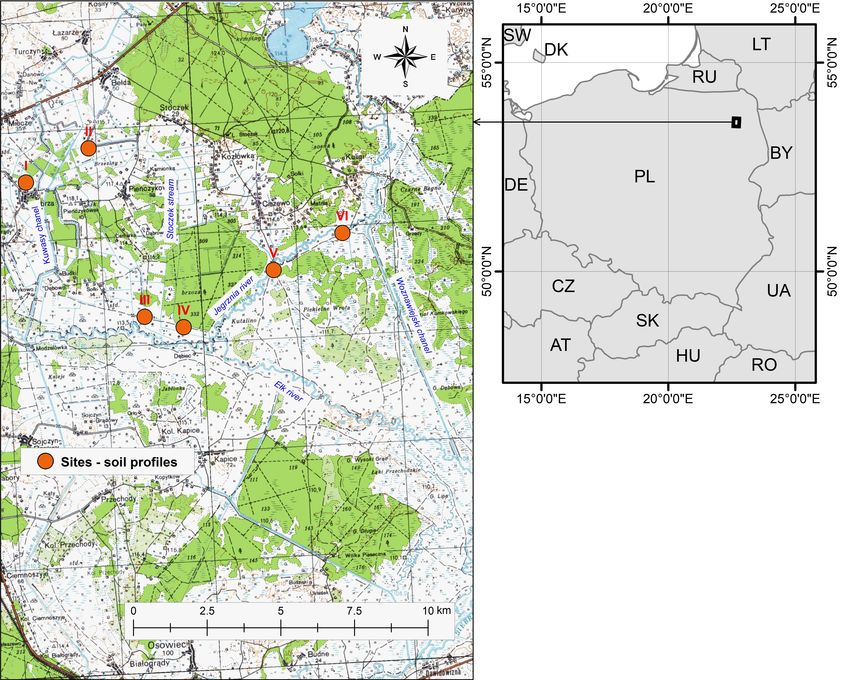
characterized by different soil properties and vegetation patches were selected (Figure 1). The term
“site” used in this study is defined as a part of the field quarter covered by representative and
relatively homogenous vegetation patches. All the studied sites were used as meadows. Two sitesWater 2018, 10, 1842 4 of 22
were located near Biebrza Village (site I and II) and the soil profiles were developed from alder peat.
Next, two profiles were situated near the Stoczek Stream (III, IV) where soil upper layers had evolved
from sedge-reed peat deposits. The last two experimental sites (V, VI) were located at the border of the
Kuwasy system near the Jegrznia River. The reed peat was the parent material of these soil profiles.
The underlying peat soil layers (below 15 cm) in sites I and II were classified as sapric Histosols horizons
whereas peats from the other soil profiles were classified as hemic Histosols [56]. The upper layers
(up to 15 cm) of the studied soils were formed as a result of long-term water table lowering. Land
drainage resulted in the soil mucky process which in turn led to developing a new organic soil material
with specific chemical, physical and biological properties [57]. The surface layers are often referred to
as muck (moorsh) material [58].
Figure 1. Location of study sites (based on http://mapy.geoportal.gov.pl).
2.2. Field Measurements and Basic Soil Properties
The set of field data was collected during 23 field campaigns conducted between 2008 and 2016
for sites I, III–VI, and 12 field campaigns during the vegetation seasons between 2006 and 2007 for
site II. During the measurement dates at the selected sites, a soil pit was dug to the depth limited by
the ground water table position. The measurements were done in the top layers (0–15 cm) recognized
as the surface soil layers dominated by moorsh material. The dielectric constant was measured in
the soil profiles at three locations spaced horizontally by 30 cm at three different depths: 5, 7.5 and
12.5 cm. A slightly different measurement methodology was applied at site II, where measurements
were conducted at a depth of 10 cm. In each measurement spot, the two rods of a TDR probe
(10 cm long) were installed horizontally for recording the dielectric constant. The TDR probe was
a part of the measurement system (field operator meter), which also comprises the pulse generatorWater 2018, 10, 1842 5 of 22
module producing a Gaussian needle pulse, with rises/falls at about 200 ps [59]. After the dielectric
constant measurements, the soil profiles were sampled for laboratory determination of gravimetric soil
water content and soil bulk density. Undisturbed soil samples were collected into horizontally-oriented
plastic cores (5.4 cm diameter and 11.8 cm height, 270 cm3 volume), coaxially inserted in the place of
Ka measurements. The collected soil cores were sealed with a rubber cover at both ends and packed
into thermal plastic bags to avoid water loss through evaporation and stored in a cooler at 4 ◦ C until
laboratory tests were conducted. In laboratory conditions, each soil sample was weighed and was
oven dried at 105 ◦ C for 24 h after air drying. Soil bulk density was calculated by dividing the oven-dry
sample weight by the core volume. Gravimetric moisture content was calculated for each sample and
then converted to volumetric moisture content by multiplying the gravimetric moisture content by soil
bulk density. In total, 278 measurements regarding the soil moisture content, soil bulk density and
dielectric constants were obtained (the measurement data for each site are shown in Table 1).
Additionally, in the laboratory conditions, the average ash content (AC) for each soil depth was
determined using the ignition method. For this reason, the disturbed sub-samples (the number of
samples are shown in Table 1) were ignited in a muffle furnace at 550 ◦ C for 4 h. The specific soil
particle density (ρp ) of the analyzed upper layers of six soil profiles was calculated assuming that an
increase of ash content of about 1% causes an increase of the ρp parameter of about 0.011 g cm−3 with
respect to the nominal value equal to 1.451 g cm−3 [60,61].
Table 1. Basic soil properties of mucky layers.
Particle
Actual Soil Bulk Density Ash Content Porosity
Sites N1 1 N2 1 Density
(g cm−3 ) (%) (g cm−3 ) (cm3 cm−3 )
Mean Min Max SD 2 Mean SD 2 Mean Mean
I 81 0.3025 0.2256 0.3883 0.0349 26 14.91 1.72 1.6150 0.8127
II 23 0.3123 0.2770 0.3540 0.0199 6 16.75 1.15 1.6353 0.8090
III 45 0.3541 0.2830 0.4271 0.0338 26 18.79 0.82 1.6577 0.7864
IV 27 0.3432 0.3102 0.3780 0.0174 9 18.42 0.86 1.6536 0.7925
V 51 0.2968 0.2211 0.3680 0.0310 16 17.94 0.93 1.6483 0.8199
VI 51 0.3082 0.2361 0.3712 0.0331 17 18.69 1.95 1.6566 0.8140
1 N1, N2—measurement numbers of actual soil bulk density and ash content respectively. 2 SD—standard deviation of
selected basic properties.
2.3. Soil Water Retention Characteristics
The undisturbed soil samples (standard volume 100 cm3 ) were collected in three replications from
the top layers (at depth 7.5 cm) of the six studied peat-muck soil profiles in order to determine soil
water retention characteristics (pF curves). The moisture content values in the range of predefined
matric potential from 0.4 to 2 pF were determined on a sand table, whereas the amount of water
retained at pF: 2.2, 2.5, 2.7, 3.4 and 4.2 was measured in pressure chambers [62]. The pF curves for each
soil profile are represented in this study by average values of moisture content at nine predefined soil
matric potentials.
2.4. Botanical Composition of Plant Cover
For each of the selected sites, the detailed quantitative botanical composition of plant species was
measured in 2008 before the first cut (end of May or beginning of June). The full developed plants
were cut from four randomly selected areas of 1 m2 , each located next to the place of the soil property
measurements. The biomass samples were stored in paper bags and then the dry weight of each
species was determined in laboratory conditions. Based on the gravimetric measurements, the mass
percentage of the particular species as a total dry mass was calculated. The list of 70 vascular species
in total was made for all selected sites can be seen in Table S1. The floristic type of the meadowWater 2018, 10, 1842 6 of 22
community was determined based on the dominant species, which accounted for at least 30% of the
biomass. “Pure” types (domination of one species), “mixed” types (predomination of two species
together constituting at least 30% of the biomass) were specified. To characterize the habitat conditions
for all meadow communities, the weighted means of Ellenberg’s indices [50,52] were calculated.
The proportion (%) of vascular plants in biomass samples was multiplied by the Ellenberg index of
this species, i.e., light—L (1–9); soil moisture—F (1–12); soil acidity—R (1–9); soil nitrogen—N (1–9)
according to [45], and then the results of multiplication for all species of plant community were
summed. The value obtained was divided by 100 and, in this way, the values of individual features
for the whole community were obtained. Additionally, the species composition of each site was
characterized using the biodiversity Shannon–Weiner’s index [63,64]. The calculation results of the
Ellenberg indices (L, F, R, N) and Shannon–Weiner’s indices (H’) are presented in the Supplementary
Materials shown in Table S2.
2.5. Data Analysis
Segmented linear regression was applied to establish the relationship between the volumetric
soil moisture content (θv ) and the dielectric constant (Ka ) for all sites and the whole range of the
analyzed dataset. This type of regression is a piecewise linear model, which describes the relationship
between response and explanatory variables and is represented by at least two straight lines crossed in
a breakpoint [65]. In this study, it was assumed that the established model is continuous, including the
breakpoints (Ψ). When there is only one breakpoint, the simplest piecewise regression model can be
written as follows [66]:
θv = β0 +β1 ·Ka +e for Ka ≤ ψ, (1)
θv = β0 +β1 ·Ka +β2 (Ka −ψ)+e for Ka > ψ, (2)
or
θv = β0 +β1 ·ψ+[β1 + β2 ]·(Ka −ψ)+e for Ka > ψ, (3)
where: β0 is intercept, β1 and β1 + β2 are the slopes of the segmented lines (β2 can be interpreted as a
difference in slopes), and e values are assumed to be independent errors with a zero mean and constant
variance. The normality of e values has been tested using the Shapiro–Wilk test and the p-value
statistic. The iterative techniques included in the R segmented package [67], was applied to identify
the breakpoint (Ψ) and to fit the regression model into the collected data. The broken-line model
(segmented regression) was used to establish the general broken-line model (GBLM) and site-specific
broken-line model (SSBLM).
The root mean square error (RMSE) was used as a measure of the differences between the moisture
content predicted by a model(s) and the actually observed values. The RMSE statistic is frequently
used to evaluate different calibration curves for the TDR method [25] or for comparisons of the
empirical models dependent on different sets of explanatory variables [68]. Additionally, the bias
representing the mean difference between the expected (using the TDR calibration model) and the
measured values of soil moisture content was determined, as indicated in [22]. The t-test was used for
comparison of the statistical difference between the data subsets.
The applicability of the bioindicators for soil moisture prediction was studied using a correlation
matrix and linear regression. Moreover, we analyzed the influence of the EIV and H values on the
hydro-physical properties of the mucky soil.
Based on the results, with respect to the field soil dielectric properties and bioindicators of the site,
the model for soil moisture content determination for upper layers of degraded peatlands was proposed
in the form of: Site-specific model discontinuous (SSM-D) and site-specific model with re-fitting of ψr
value (SSM-R). The calculations were made using the RWeka package [69]. For this purpose, we used
the M5Rules algorithm [70,71] belonging to the regression tree method. The basic assumption of this
type of algorithm is dividing the entire set of samples by selecting one independent input variable
among all and then performing the binary split into at least two child sets, which should increaseWater 2018, 10, 1842 7 of 22
the purity of the data compared with its single parent node [72]. The nodes which cannot be further
partitioned are called leaves. After growing the tree and the pruning process (removing the leaf with
insignificant influence on purity) the linear regression can be fitted for the growing leaf in order to
improve the fit of the model [70,73]. The tree construction process, as described above, provides
an approximation of function specific for each final node which can lead to sharp discontinuities
occurring between adjacent leaves and requires smoothing of the tree after the full set of rules has been
produced [74]. During the learning process, we applied a cross-validation scheme [75] to establish
the SSM-D model. We used all six possible different combinations of the data from five sites for the
training of the M5Rules algorithm, the remaining dataset was used for testing. Each analyzed dataset
included continuous variables, i.e., soil moisture content (θv ) and dielectric constant (Ka ) measured
for all investigated sites, as well as categorical covariates represented by bioindices (F, L, N, R, H’).
The M5Rules algorithm was run six times to fit the data and the best SSM-D model was selected
using the RMSE value for testing of the data. After that the SSM-D was iteratively smoothed and the
threshold value ψr and θvr was determined, finally resulting in SSM-R model determination.
3. Results and Discussion
3.1. Soil Properties and Botanical Composition of Plant Cover
Table 1 summarizes the basic soil properties represented by the measured value of soil bulk
density and ash content for the studied mucky horizons (0–15 cm). The average soil particle density as
well as the porosity of the analyzed top soil layers was calculated using the basic physical properties of
the soil.
The higher values of this feature compared to peat soils can be attributed to the intensive
cultivation practice and soil compaction. Despite cultivation differences of peat soils in European
countries, the analyzed average soil bulk density values (ρb ) in the upper layers were comparable
with peat soils agriculturally cultivated in England [76], Sweden [77], Norway [78] and Germany [79].
The ash content in the analyzed mucky soil was low and this results from the lack of temporary river
flood conditions on the selected sites during moorsh soil development. The average porosity of the
studied moorsh horizons was lower, approximately 0.05 to 0.10 cm3 cm−3 compared to the underlying
original peat deposits [40,42,61].
The mucking process therefore, apart from the basic physical property changes of the soil, seriously
affected the soil moisture retention characteristics (Table 2). The presented pF curves of the mucky soils
are characterized by a relatively low amount of gravitational water (the difference between porosity
and soil moisture content at pF = 2.0) compared to the peat soils.
Table 2. Average soil moisture content at predefined soil matric potentials pF.
Soil Moisture Content at Predefined Soil Matric Potentials pF (cm3 cm−3 )
Sites
pF = 0.4 pF = 1.0 pF = 1.5 pF = 2.0 pF = 2.2 pF = 2.5 pF = 2.7 pF = 3.4 pF = 4.2
I 0.803 0.783 0.728 0.645 0.606 0.564 0.547 0.385 0.309
II 0.808 0.799 0.786 0.694 0.660 0.608 0.571 0.441 0.360
III 0.775 0.758 0.730 0.649 0.599 0.553 0.530 0.379 0.330
IV 0.790 0.774 0.727 0.677 0.576 0.502 0.476 0.356 0.303
V 0.819 0.812 0.724 0.616 0.559 0.521 0.504 0.335 0.248
VI 0.802 0.750 0.723 0.658 0.612 0.583 0.562 0.393 0.343
Values of Basic Statistics
Mean 1 0.7995 0.7793 0.7363 0.6565 0.6020 0.5552 0.5317 0.3815 0.3155
SD 2 0.0152 0.0237 0.0245 0.0270 0.0347 0.0391 0.0362 0.0361 0.0392
CV 3 1.90 3.04 3.33 4.11 5.76 7.04 6.81 9.46 12.42
1 mean—arithmetic average (cm3 cm−3 ). 2 SD—standard deviation (cm3 cm−3 ). 3 CV—coefficient of variation (%).Water 2018, 10, 1842 8 of 22
In the present study, these soil water retention indicators were in the range between 0.11 and
0.20 cm3 cm−3 , whereas in the study of [42], in the peat soils, the amount of gravitational water
was higher and equal to approximately 0.34 cm3 cm−3 . However, the soil moisture content at the
permanent wilting point (pF = 4.2) of the studied mucky layers was relatively high and remains in the
same range as in the peat soils [42]. The obtained results of hydro-physical properties of the mucky
layers show an increment of mineral compounds in the soil matrix compared to the peat soils, which
indicates that the structure of this organic material dramatically changed due to drainage [80] and
cultivation practice, and evolved from fibrous into a grainy or humic structure [61].
The plant communities have been classified in the five floristic types, two “pure” (II, V–VI sites)
and three “mixed” (Table 3). I, V and VI sites were characterized by the predominant occurrence of
low grasses mainly Festuca rubra, and at site VI also sedge (Carex panicea).
Table 3. The habitat conditions and the Shannon–Weiner’s index of the meadow communities in the
examined sites (mean values).
Ellenberg’s Indices
Sites H’ 5 Floristic Type
L1 F2 R3 N4
I 4.96 5.62 2.39 4.34 2.26 Poa pratensis + Festuca rubra
II 6.80 6.22 4.43 6.29 2.09 Phalaris arundinacea
III 5.50 5.03 1.03 3.32 2.18 Holcus lanatus + P. pratensis
IV 6.37 5.12 2.83 4.27 2.43 Achillea millefolium + Odontites serotina
V 3.43 5.03 3.35 2.00 2.24 F. rubra
VI 3.14 5.50 3.21 1.50 1.50 F. rubra
1 L—light. 2 F—soil moisture. 3 R—soil acidity. 4 N—soil nitrogen 5 H’—Shannon–Weiner’s index.
The Shannon–Wiener index in the analyzed plant communities was moderate [48] and oscillates
(apart from site VI) in the range from 2.09 to 2.43. VI site was characterized by low diversity indices
mainly because of the lowest number of species (20 species) and the predominance of two main species
(about 73% of biomass). The highest values of the EIV measures were noted for the II site. The floristic
composition of plant communities of the studied sites indicates the diversity of ecological conditions of
the habitats (Table 3) thereby confirming the assumptions formulated in the materials and methods
section focusing on the biological diversity of the plant cover.
3.2. Analysis of Existing Relationships between Dielectric Constant and Soil Moisture Content in Organic Soils
The relationship between the measured soil moisture content and the dielectric constant in
respect to the field site is presented in Figure 2. Data are illustrated together with the TDR calibration
curves for peat soils available in the literature listed in Table 4. A simple graphical inspection of the
presented features indicates that any of the applied calibration equations do not fit the whole range of
our dataset. The best prediction of the TDR soil moisture content for moorsh soil from the Biebrza
River Valley can be approximated using equations P4 and PS2 [22].
The RMSE for these models was nearly 0.06 cm3 cm−3 . Despite the reasonably good results of
the RMSE statistic, the mentioned equations gave a satisfactory prediction of soil moisture content at
different ranges of dielectric constant changes. The most appropriate literature model P4 enabled a
reasonably good approximation of the soil moisture content in the range of dielectric constant between
10 and 20. The highest overestimation of soil moisture content (of about 0.15 cm3 cm−3 ) occurred
when the dielectric constant was equal to 30. Figure 2 also shows the measured data of the soil
moisture content and the dielectric constant and their fitting using the logarithmic model (NL_own)
The following form of equation was obtained:
θv = 0.2417· ln(Ka )−0.2173. (4)conditions of the habitats (Table 3) thereby confirming the assumptions formulated in the materials
and methods section focusing on the biological diversity of the plant cover.
3.2. Analysis of Existing Relationships between Dielectric Constant and Soil Moisture Content in Organic Soils
The10,
Water 2018, relationship
1842 between the measured soil moisture content and the dielectric constant in
9 of 22
respect to the field site is presented in Figure 2. Data are illustrated together with the TDR calibration
curves for peat soils available in the literature listed in Table 4. A simple graphical inspection of the
The calculated 3 cm−3 ) in comparison to the P4 and
presented features RMSE
indicatesvalue
thatwas
anyessentially lowercalibration
of the applied (0.0452 cmequations do not fit the whole range
PS2 models.
of our However,
dataset. The bestEquation (4) of
prediction overestimated
the TDR soilthe moisture
moisture content
content forby as much
moorsh soilasfrom
0.15the cm−3
cm3Biebrza
in the middle
River range
Valley can beof the dielectricusing
approximated constant changes.
equations P4 and PS2 [22].
Figure2.2.Measured
Figure Measureddata
dataofofdielectric
dielectricconstant
constantand
andsoil
soilmoisture
moisturecontent
contentfor
fordifferent
differentsites
sitestogether
together
with own empirical relationship (NL_own) and relationships listed in Table
with own empirical relationship (NL_own) and relationships listed in Table 4. 4.
Table 4. Selected literature calibration models for time domain reflectometry (TDR) methods and root
mean square error (RMSE) statistics with respect to all collected dataset, as well as for data of the “dry”
and “wet” segment of the general broken-line model (GBLM).
Root Mean Square Error
RMSE (cm3 cm−3 )
Calibration θv Ka Independent
NO Soil Function Overall Segments of
Models Range Range Variable
Range GBLM Model
of Data “dry” “wet”
1 P1 [23] O 0.03–0.55 ~3–35 Ka p 0.4262 0.0924 0.5015
2 P2 [29] SM 0.20–0.90 ~5–60 Ka p 0.0704 0.0764 0.0678
3 P3 [30] O 0.00–0.75 ~1–60 Ka p 0.0748 0.1097 0.0546
4 P4 [31] SC 0.30–0.80 ~10–65 Ka p 0.0571 0.0797 0.0448
5 P5 [32] B 0.60–0.90 ~29–75 Ka p 0.1130 0.1672 0.0815
6 PS1[33] SM 0.00–0.98 ~3–75 sqrt (Ka ) p 0.1090 0.1364 0.0957
7 PS2 [33] SM 0.00–0.98 ~3–75 sqrt (Ka ) p 0.0586 0.0789 0.0480
8 LS1 [81] O 0.10–0.80 ~2–40 sqrt (Ka ) l 0.0958 0.0666 0.1053
9 LS2 [82] Fo 0.00–0.70 ~1–40 sqrt (Ka ) l 0.0908 0.0643 0.0996
10 LS3 [83] SM 0.00–0.95 ~2–73 sqrt (Ka ) l 0.0653 0.0801 0.0582
11 NL_own * Mu 0.22–0.81 6–61 ln(Ka ) nl 0.0452 0.0586 0.0385
12 GBLM * Mu 0.22–0.81 6–61 Ka ls 0.0405 0.0508 0.0356
θv —volumetric soil moisture content (cm3 cm−3 ); Ka —dielectric constant (-); p—polynomial, l—linear;
nl—nonlinear; ls—segmented linear; *—this study; O-organic soils, SC—Sphagnum, Carex peat SM-Sphagnum
moss, B—blanket peat; Fo—forest soils, Mu—muck soils.
3.3. General and Site-Specific Relationships between Dielectric Constant and Soil Moisture Content
Based on the graphical inspection and simple statistical analysis, we decided to select the
continuous broken-line model as an approximation to describe the non-linear relationship between
soil moisture content and dielectric constant of the mucky soil (for all measured data of θvWater 2018, 10, 1842 10 of 22
and Ka ). For this purpose, the segmented linear regression was applied and the model parameters
(Equations (1) and (3)) were estimated iteratively [67]. The results of the statistical computation
indicated that the established continuous general broken-line model (GBLM) included one threshold
parameter (Ψ), and can be written as:
θv = 0.2335 + 0.01178·Ka for Ka ≤ ψ, (5)
θv = 0.2335 + 0.01178·Ka −0.0046·(Ka −ψ) for Ka > ψ. (6)
After rearrangement the Equation (6) can be written in its final form as follows:
θv = 0.2335 + 0.01178·ψ + 0.007179·(Ka −ψ) for Ka > ψ. (7)
The break-point (Ψ) for the analyzed dataset was determined for Ka equal to 31.49 (Figure 3).
The 95% confidence interval for this parameter was wide and ranged from 27.22 to 35.76 (Figure 3).
Residuals from the model (Equations (5) and (6), or (5) and (7)) were normally distributed around the
average which was confirmed by the Shapiro–Wilk testing statistic (W = 0.9919) and the p-value (0.1302).
The RMSE value for the GBLM equations equals to 0.0405 cm3 cm−3 and is essentially lower than
the estimates determined for the equations indicated in Table 4. This type of broken-line relationship
is often usedWater
to assess thePEER
2018, 10, x FOR threshold
REVIEW value where the effect of the covariate changes. 10 of In
21 the fields of
hydrology and soilwhich
average hydrology, the piecewise
was confirmed linear regressions
by the Shapiro–Wilk testing statistic(PLR) and the
(W = 0.9919) and determined
the p-value threshold
values are used to explain
(0.1302). The RMSE the influence
value of the
for the GBLM vegetation
equations equals tocover
0.0405 fraction onisthe
cm3 cm−3 and reduction
essentially lower of runoff [84]
than the estimates determined for the equations indicated in Table 4. This type of broken-line
and the erodibility coefficient [85]. In the water study, the two-segmented broken-line equation is
relationship is often used to assess the threshold value where the effect of the covariate changes. In
applied for predicting water and
the fields of hydrology electrical conductivity
soil hydrology, the piecewiseusing a portable
linear regressions X-ray
(PLR) fluorescence
and the determined meter [86].
The meaningthreshold
of a break-point in to
values are used this study
explain the of the TDR
influence of thecalibration curve
vegetation cover canonbetheexplained
fraction reduction as the point
of runoff [84] and the erodibility coefficient [85]. In the water study, the two-segmented broken-line
depending on the soil water retention characteristic (horizontal lines on Figure 4). The threshold value
equation is applied for predicting water electrical conductivity using a portable X-ray fluorescence
(Ψ) with the meter
confidence
[86]. Theinterval
meaning ofin general was
a break-point included
in this study of thebetween horizontal
TDR calibration curve canlines which indicated the
be explained
moisture contents at matric
as the point potential
depending between
on the soil pF values
water retention from 2.0
characteristic to 2.7.lines
(horizontal Theonaverage
Figure 4).moisture
The content
threshold value (Ψ) with3 the confidence
− 3 interval in general was included between horizontal lines
at break point (θψ = 0.6044 cm cm ) was approximately equal to soil moisture content at pF = 2.2
which indicated the moisture contents at matric potential between pF values from 2.0 to 2.7. The
(θv = 0.6020 cm 3 cm−3 ). The validity of the threshold value can be approximately
explained by bulk
average moisture content at break point (θψ = 0.6044 cm3 cm −3) was equal to density
soil changes
(Figure 4). moisture content at pF = 2.2 (θv = 0.6020 cm3 cm−3). The validity of the threshold value can be explained
by bulk density changes (Figure 4).
Figure 3. Field measurements and fitted GBLM for the relationship between soil moisture content and
Figure 3. Field measurements and fitted GBLM for the relationship between soil moisture content and
dielectric constant. The horizontal dotted black lines indicate the soil moisture content at predefined
dielectric constant. The horizontal
pressure head. dotted
The red vertical black the
line indicates lines indicate
average value the soil
of the moisture
breaking point content
(ψ = 31.49)at predefined
pressure head. Thethered
whereas vertical
red dotted linelineindicates
vertical the average
is the 95% confidence value of the breaking point (ψ = 31.49)
interval.
whereas the red dotted vertical line is the 95% confidence interval.
The soil bulk density of the two segments was statistically different. For the “wet” range
(segment wet above the threshold Ψ), the average bulk density was equal to 0.31 g cm−3, whereas at
the “dry” range (segment dry) its estimates are equal to 0.33 g cm−3. It can be concluded that below
the breakpoint of the θv(Ka) characteristic, the significant increase of bulk density indicates the
essential soil volume changes. The field study conducted for similar soils confirmed that, apart from
the soil moisture contents changes [87], the soil bulk density also changes in space and time [40].
Despite improvements in the GBLM model in comparison to the literature equations, the bias of theWater 2018, 10, 1842 11 of 22
The soil bulk density of the two segments was statistically different. For the “wet” range (segment
wet above the threshold Ψ), the average bulk density was equal to 0.31 g cm−3 , whereas at the
“dry” range (segment dry) its estimates are equal to 0.33 g cm−3 . It can be concluded that below the
breakpoint of the θv (Ka ) characteristic, the significant increase of bulk density indicates the essential
soil volume changes. The field study conducted for similar soils confirmed that, apart from the soil
moisture contents changes [87], the soil bulk density also changes in space and time [40].
Despite improvements in the GBLM model in comparison to the literature equations, the bias of
the calibration equation depends on site-specific data measurements of θv (Ka ). The segmented model
gave a weak prediction of the soil moisture content for site II (bias equal to approximately 0.044 cm3 cm−3 )
as well as in the dry range of the soil moisture content in sites VI, V and IV.
Water 2018, 10, x FOR PEER REVIEW 11 of 21
Figure 4.Figure 4. Boxplot
Boxplot of soilofbulk
soil bulk density
density forfor “dry”and
“dry” and “wet”
“wet” segments
segments of the measured
of the datasetdataset
measured (dotted (dotted
line indicates overall average soil bulk density). The scattered point indicates the soil bulk density
line indicates overall average soil bulk density). The scattered point indicates the soil bulk density
value with respect to sites. The dotted horizontal line indicates the overall soil bulk density average.
value with respect to sites. The dotted horizontal line indicates the overall soil bulk density average.
The diamond symbol indicates the average soil bulk density for each segment of the dataset. The red
The diamond symbol
dots indicate theindicates
outliers. the average soil bulk density for each segment of the dataset. The red
dots indicate the outliers.
The analysis of the GBLM model limitations forced us to develop the site-specific broken-line
Themodel (SSBLM).
analysis of theFor this purpose,
GBLM model the linear regression
limitations forcedlinesus to were fitted for
develop thethe analyzed sites
site-specific in
broken-line
respect to data below and above the threshold value (Figure 3). The obtained
model (SSBLM). For this purpose, the linear regression lines were fitted for the analyzed sites in slopes (β 1, β1 + β2) and
intercepts (β0) enabled the calculation of the breakpoint value separately for the soil from the specific
respect to data below and above the threshold value (Figure 3). The obtained slopes (β1 , β1 + β2 ) and
sites. The parameters of the SSBLM models are summarized in Table 5.
intercepts (β0 ) enabled the calculation of the breakpoint value separately for the soil from the specific
sites. The parameters of 5.
Table the SSBLM broken-line
Site-specific models are summarized
model parameters (SSBLM)in Table 5. TDR method.
for the
Fitted lines below the threshold β0 (“dry” range) β1 wereβcharacterized
1 + β2 Ψ by similar θΨ slope values (average
Sites
value equal to 0.0136 and CV =(cm6.31%).
3 cm−3) In (cm
the3 “wet”
cm−3) range,
(cm3 cm slopes
−3) (β(-)1 + β2(cm
) were
3 cm−3generally
) flatter than
in the “dry” range (β1 ) Iand relatively 0.2157more variable
0.0125 (CV = 24%) mainly
0.00800 27.42 because 0.5585of the lowest slope of
the θv (Ka ) relationship II for site II. 0.2456
Except for this 0.0129
site, the0.00380 35.25
slope parameters in 0.7003
the “wet” range were also
not essentially different. The Ψ parameter represents a wide range of changes0.5866
III 0.1941 0.0144 0.00660 27.26
in the dielectric constant
IV 0.2587 0.0133 0.00640 18.29 0.5020
(Table 5) which directlyVinfluences the really 0.0139
0.1330
wide scatter of the soil
0.00810
moisture0.6192
34.98
content (θΨ ) estimated at
break point (Ψ). Despite VI the low 0.0740
CV value, the moisture0.00613
0.0147 content at the break0.6935
42.14 points (θΨ ) ranged from
0.50 to 0.70 cm3 cm−3 which represents aValues relatively wide
of basic scatter for this type of soil. The comparison of
statistics
θΨ values with the range Mean 1of moisture
0.1869 content 0.01362
of pF curves0.00651 30.89 that the
indicated 0.6100
threshold values were
SD 2 0.0709 0.00086
included in the range of the soil matric potential approximately between pF 0.00157 8.32 0.0776
= 2.0 (site II) to pF = 2.5
CV 3 37.93 6.31 24.12 26.93 12.72
(site IV). 1 mean—arithmetic average. SD—standard deviation. CV—coefficient of variation (%).
2 3
Fitted lines below the threshold (“dry” range) were characterized by similar slope values
(average value equal to 0.0136 and CV = 6.31%). In the “wet” range, slopes (β1 + β2) were generally
flatter than in the “dry” range (β1) and relatively more variable (CV = 24%) mainly because of the
lowest slope of the θv(Ka) relationship for site II. Except for this site, the slope parameters in the “wet”
range were also not essentially different. The Ψ parameter represents a wide range of changes in theWater 2018, 10, 1842 12 of 22
Table 5. Site-specific broken-line model parameters (SSBLM) for the TDR method.
β0 β1 β1 + β2 Ψ θΨ
Sites
(cm3 cm−3 ) (cm3 cm−3 ) (cm3 cm−3 ) (-) (cm3 cm−3 )
I 0.2157 0.0125 0.00800 27.42 0.5585
II 0.2456 0.0129 0.00380 35.25 0.7003
III 0.1941 0.0144 0.00660 27.26 0.5866
IV 0.2587 0.0133 0.00640 18.29 0.5020
Water 2018, 10, x FOR
V PEER REVIEW
0.1330 0.0139 0.00810 34.98 0.6192 12 of 21
VI 0.0740 0.0147 0.00613 42.14 0.6935
dielectric constant (Table 5) which directly influences the really wide scatter of the soil moisture
Values of basic statistics
content (θΨ) estimated at break point (Ψ). Despite the low CV value, the moisture content at the break
Mean 1 0.1869 0.01362 0.00651 30.89 0.6100
points (θΨ) ranged
SD 2 from 0.50
0.0709to 0.70 cm 3 cm−3 which represents a relatively wide scatter for this type
0.00086 0.00157 8.32 0.0776
of soil. The comparison
CV 3 of37.93
θΨ values with the range of24.12
6.31 moisture content
26.93 of pF curves
12.72indicated that
the threshold values were included
1 mean—arithmetic in2 the range of the soil
3 matric potential approximately
average. SD—standard deviation. CV—coefficient of variation (%). between
pF = 2.0 (site II) to pF = 2.5 (site IV).
Figure5 5shows
Figure showsthethemeasured
measureddata dataofof the
the soil
soil moisture
moisture content
content and
and the
the dielectric
dielectric constant
constant forfor
the
the specific sites and their fitting using the segmented model (SSBLM) and the logarithmic
specific sites and their fitting using the segmented model (SSBLM) and the logarithmic equations (NL equations
(NL type).
type).
Figure
Figure5.5.Field
Fieldmeasurements
measurementsandandfitted
fitted models
models of of the relationshipbetween
the relationship betweenthe thesoil
soilmoisture
moisturecontentcontent
and
anddielectric
dielectricconstant
constantfor
forspecific
specific sites.
sites. (a)
(a) Site
Site I;
I; (b) site II;
(b) site II; (c)
(c) site
site III;
III;(d)
(d)site
siteIV;
IV;(e)
(e)site
siteV;V;(f)(f)site
siteVI.
VI.
The
TheSSBLM
SSBLMmodelmodeldeveloped
developedseparately
separately for the soils from
from different
differentsites
sitesindicates
indicatesthe
thereasonably
reasonably
good
goodresults
resultsofof
fitting in in
fitting all all
ranges of the
ranges θv(K
of the θav)(K
relationship changes.
a ) relationship The RMSE
changes. The RMSEvalues were were
values varied
varied depending
depending on the site on data.
the siteFordata. For the calibration
the calibration curves
curves from from
sites III,sites III, VI,
V and V and
the VI, the values
values did not
exceed 0.03 cm3 cm−3. The RMSE values for the rest of the developed SSBLM equations were slightly
higher and varied from 0.036 cm3 cm−3 (site I) to 0.041 cm3 cm−3 (site IV). It should be stressed that
logarithmic type models developed for specific site were less accurate and the RMSE value was
generally higher (of about 0.005 to 0.012 cm3 cm−3) in comparison to the SSBLM models. The
logarithmic models underestimated the soil moisture content by as much as 0.07 cm3 cm−3 in the wetWater 2018, 10, 1842 13 of 22
did not exceed 0.03 cm3 cm−3 . The RMSE values for the rest of the developed SSBLM equations
were slightly higher and varied from 0.036 cm3 cm−3 (site I) to 0.041 cm3 cm−3 (site IV). It should be
stressed that logarithmic type models developed for specific site were less accurate and the RMSE
value was generally higher (of about 0.005 to 0.012 cm3 cm−3 ) in comparison to the SSBLM models.
The logarithmic models underestimated the soil moisture content by as much as 0.07 cm3 cm−3 in the
wet range of calibration curve. From this reason for further analysis, we applied broken-line model
parameters as an approximation of the non-linear relationship between Ka and θv .
3.4. Applicability Analysis of the Bio-Indices in Soil Moisture Prediction and Hydro-Physical Properties of
Mucky Soils
Feasibility analysis of the calibration model development for the moorsh moisture content
prediction as a function of dielectric constant with the participation of the covariates represented by
bioindices is illustrated using the correlation coefficients (Figure 6).
The broken-line model parameters (Table 5) were correlated with the bioindices (Table 3).
The highest correlation coefficient has been noted between intercept (β0 ) and indicator L of the
Ellenberg scale. However, the β0 also correlates with “productivity” of the ecosystem (N) as well as
with the Shannon–Weiner index (H’). The slope in the “dry” range of the calibration curves (β1 )
was strongly but negatively correlated with “productivity” of the ecosystem (N) determined on the
basis of the plant cover as well as positively correlated with the ash content (AC) of the analyzed
soils. Nevertheless, both of the explained covariates (AC and N) were moderately and negatively
correlated, which can suggest that the increase of the AC amount in the soil causes reduction of the
“productivity” of the analyzed ecosystems. The slope in the “wet” range of the calibration curves
(β1 + β2 ) can be approximated using the soil moisture substrate indicator (F), which in the case of our
studied sites describes fresh soil with moderate wetness [51]. Due to the low range of the F indicator
changes and moderate variation of the β1 + β2 parameter, the prediction of the slope in the “wet”
range of the calibration curve can be more complex than simple application of the linear relationship.
The estimation of this parameter is especially important for the organic soils where soil moisture
changes in the wet range strongly influence the soil degradation processes and physical soil properties.
On the other hand, the β1 + β2 parameters were highly correlated with soil pF curve characteristics.
From the data presented in Figure 6, it can be observed that these parameters were also negatively
correlated with soil moisture contents measured at the predefined soil matric potentials ranging from
pF = 1.5 to pF = 4.2. Moreover, it should be stressed that the moisture of the soil substrate (indicator F)
was also highly correlated with the moisture content of the pF curves (Figure 6) which, in general,
is in agreement with the statements made in [50]. Based on the correlation analysis, it can be noted
that the slope in the “wet” range of the field calibration curves can be fairly well determined using the
moisture indicator of the Ellenberg scale, or more precisely using the soil moisture content at pF = 2 as
a soil type (site) specific predictor.
The broken-line model parameter Ψ was correlated with bioindicators of soil cover, physical soil
properties and soil water retention characteristic. The highest r value was determined between Ψ and
the Shannon–Weiner index. This could suggest that the variety of the plant species, which are typical
for the site location, influences the slope separation point of the TDR calibration curves. This was
especially visible in the case of two sites: VI and IV. In the former, the Ψ value was the highest and
soil cover is mainly occupied by two plant species (Festuca rubra and Carex panicea) which affected the
lowest value of the H’ index. On the other hand, at site IV the highest H’ value was observed (2.4)
which indicates a condition of greater biodiversity (with a predominance of dicotyledonous plants),
however, the Ψ value was the lowest (18.29). Although the Ψ value is was highly correlated with
the Shannon–Weiner index, its value can also be carefully approximated by physical soil properties.
Our data indicate that the increase of Ψ value was related to the increase of average soil porosity and
soil moisture status at pF = 2.5 and 2.7. The Ψ value was also highly correlated with the ratio betweencharacteristics. From the data presented in Figure 6, it can be observed that these parameters were
also negatively correlated with soil moisture contents measured at the predefined soil matric
potentials ranging from pF = 1.5 to pF = 4.2. Moreover, it should be stressed that the moisture of the
soil substrate (indicator F) was also highly correlated with the moisture content of the pF curves
Water 2018, 10, 1842 14 of 22
(Figure 6) which, in general, is in agreement with the statements made in [50]. Based on the
correlation analysis, it can be noted that the slope in the “wet” range of the field calibration curves
can beL fairly
and F value suggesting anusing
well determined importance of light and
the moisture moisture
indicator ofbioindicators
the Ellenbergin determination of precisely
scale, or more the
threshold value of the TDR calibration curve.
using the soil moisture content at pF = 2 as a soil type (site) specific predictor.
Water 2018, 10, x FOR PEER REVIEW 14 of 21
The broken-line model parameter Ψ was correlated with bioindicators of soil cover, physical soil
properties and soil water retention characteristic. The highest r value was determined between Ψ and
the Shannon–Weiner index. This could suggest that the variety of the plant species, which are typical
for the site location, influences the slope separation point of the TDR calibration curves. This was
especially visible in the case of two sites: VI and IV. In the former, the Ψ value was the highest and
soil cover is mainly occupied by two plant species (Festuca rubra and Carex panicea) which affected the
lowest value of the H’ index. On the other hand, at site IV the highest H’ value was observed (2.4)
which indicates a condition of greater biodiversity (with a predominance of dicotyledonous plants),
however, the Ψ value was the lowest (18.29). Although the Ψ value is was highly correlated with the
Figure 6. Correlation
Shannon–Weiner
Figure graph
index,
6. Correlation its
graph of of
valuethe analyzed
can
the variables.
also be carefully
analyzed Arrowsinin
variables. approximated
Arrows green
green by and
red red
physical
and indicate
soil
indicate statistically
properties.
statistically Our
significant
data indicatepositive
significantthat and
the
positive negative
increase
and of correlations.
negative value was Dark
Ψcorrelations. relatedyellow
to the
Dark yellow arrows
increase
arrows indicate
not not
of average
indicate statistically
soil porosity
statistically significant
and soil
significant
moisture status
TheatThe
correlations.
correlations. pFlabelled
= 2.5cells
labelled and 2.7.
cells The statistically
indicate
indicate Ψstatistically
value wassignificant
also highly
significant correlated
correlation withdifferent
between
correlation between the different
ratiotypes
between
of
typesLof
and Fvariables
variablesvalue regarding
regarding thethe
suggesting anstate
state ofof thehabitats,
importance
the habitats, SSBLM
of light
SSBLMandand soil
moisture
and soilhydro-physical properties.
bioindicators
hydro-physical in determination of the
properties.
threshold value of the TDR calibration curve.
Figure 7a–d shows simple regression lines allowing prediction of the broken-line model
Figure 7a–d shows simple regression lines allowing prediction of the broken-line model
parameters (Equations (1) and (3)) using bioindices (L, F, N, H’) determined on the basis of the
parameters (Equations (1) and (3)) using bioindices (L, F, N, H’) determined on the basis of the
measured plant
measured plant species’
species’ composition
composition for for the
the selected
selected sites.
sites.
Figure
Figure 7.
7. Linear
Linear regression
regression lines
lines between
between parameters
parameters of of the
the broken-line
broken-line model
model andand explanatory
explanatory
variables: (a) the Ellenberg index L - light vs. the intercept β 0 of SSBLM; (b) the Ellenberg index
variables: (a) the Ellenberg index L - light vs. the intercept β0 of SSBLM; (b) the Ellenberg index N –
N – productivity
productivity vs. slope
vs. the the slope
β1 of of SSBLM;
β1SSBLM; (c) the
(c) the Ellenberg
Ellenberg indexindex
F–F – moisture
moisture vs. vs.
the the slope
slope β1 +β1β+2 βof2
of SSBLM; (d) the biodiversity index – H’ vs. the breakpoint (Ψ)
SSBLM; (d) the biodiversity index – H’ vs. the breakpoint (Ψ) of SSBLM. of SSBLM.
3.5. Calibration Model Development of Soil Moisture Content as a Function of Dielectric Constant and
Botanical Indices of Soil Cover Using the Regression Tree Method
Based on the discussion presented in Section 3.4, we can state that the development of the
general calibration curve for predicting moorsh moisture content using the TDR method for a specificYou can also read


