Object Detection with Discriminatively Trained Part Based Models
←
→
Page content transcription
If your browser does not render page correctly, please read the page content below
1
Object Detection with Discriminatively Trained
Part Based Models
Pedro F. Felzenszwalb, Ross B. Girshick, David McAllester and Deva Ramanan
Abstract—We describe an object detection system based on mixtures of multiscale deformable part models. Our system is able
to represent highly variable object classes and achieves state-of-the-art results in the PASCAL object detection challenges. While
deformable part models have become quite popular, their value had not been demonstrated on difficult benchmarks such as the
PASCAL datasets. Our system relies on new methods for discriminative training with partially labeled data. We combine a margin-
sensitive approach for data-mining hard negative examples with a formalism we call latent SVM. A latent SVM is a reformulation of
MI-SVM in terms of latent variables. A latent SVM is semi-convex and the training problem becomes convex once latent information is
specified for the positive examples. This leads to an iterative training algorithm that alternates between fixing latent values for positive
examples and optimizing the latent SVM objective function.
Index Terms—Object Recognition, Deformable Models, Pictorial Structures, Discriminative Training, Latent SVM
F
1 I NTRODUCTION it has been difficult to establish their value in practice.
Object recognition is one of the fundamental challenges On difficult datasets deformable part models are often
in computer vision. In this paper we consider the prob- outperformed by simpler models such as rigid templates
lem of detecting and localizing generic objects from [10] or bag-of-features [44]. One of the goals of our work
categories such as people or cars in static images. This is to address this performance gap.
is a difficult problem because objects in such categories While deformable models can capture significant vari-
can vary greatly in appearance. Variations arise not only ations in appearance, a single deformable model is often
from changes in illumination and viewpoint, but also not expressive enough to represent a rich object category.
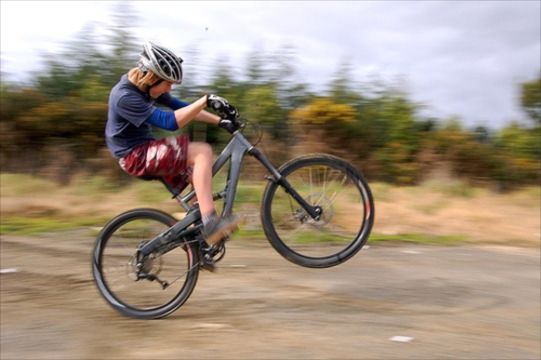
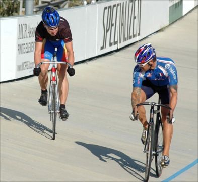
due to non-rigid deformations, and intraclass variability Consider the problem of modeling the appearance of bi-
in shape and other visual properties. For example, peo- cycles in photographs. People build bicycles of different
ple wear different clothes and take a variety of poses types (e.g., mountain bikes, tandems, and 19th-century
while cars come in a various shapes and colors. cycles with one big wheel and a small one) and view
We describe an object detection system that represents them in various poses (e.g., frontal versus side views).
highly variable objects using mixtures of multiscale de- The system described here uses mixture models to deal
formable part models. These models are trained using with these more significant variations.
a discriminative procedure that only requires bounding We are ultimately interested in modeling objects using
boxes for the objects in a set of images. The resulting “visual grammars”. Grammar based models (e.g. [16],
system is both efficient and accurate, achieving state-of- [24], [45]) generalize deformable part models by rep-
the-art results on the PASCAL VOC benchmarks [11]– resenting objects using variable hierarchical structures.
[13] and the INRIA Person dataset [10]. Each part in a grammar based model can be defined
Our approach builds on the pictorial structures frame- directly or in terms of other parts. Moreover, grammar
work [15], [20]. Pictorial structures represent objects by based models allow for, and explicitly model, structural
a collection of parts arranged in a deformable configu- variations. These models also provide a natural frame-
ration. Each part captures local appearance properties of work for sharing information and computation between
an object while the deformable configuration is charac- different object classes. For example, different models
terized by spring-like connections between certain pairs might share reusable parts.
of parts. Although grammar based models are our ultimate
Deformable part models such as pictorial structures goal, we have adopted a research methodology under
provide an elegant framework for object detection. Yet which we gradually move toward richer models while
maintaining a high level of performance. Improving
• P.F. Felzenszwalb is with the Department of Computer Science, University
performance by enriched models is surprisingly difficult.
of Chicago. E-mail: pff@cs.uchicago.edu Simple models have historically outperformed sophis-
• R.B. Girshick is with the Department of Computer Science, University of ticated models in computer vision, speech recognition,
Chicago. E-mail: rbg@cs.uchicago.edu
• D. McAllester is with the Toyota Technological Institute at Chicago. E-
machine translation and information retrieval. For ex-
mail: mcallester@tti-c.org ample, until recently speech recognition and machine
• D. Ramanan is with the Department of Computer Science, UC Irvine. translation systems based on n-gram language models
E-mail: dramanan@ics.uci.edu
outperformed systems based on grammars and phrase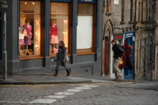
2

structure. In our experience maintaining performance
seems to require gradual enrichment of the model.
  One reason why simple models can perform better in
practice is that rich models often suffer from difficulties
in training. For object detection, rigid templates and bag-
of-features models can be easily trained using discrimi-
native methods such as support vector machines (SVM).
Richer models are more difficult to train, in particular
because they often make use of latent information.
   Consider the problem of training a part-based model
from images labeled only with bounding boxes around
the objects of interest. Since the part locations are not
labeled, they must be treated as latent (hidden) variables
during training. More complete labeling might support
better training, but it can also result in inferior training
if the labeling used suboptimal parts. Automatic part
labeling has the potential to achieve better performance
by automatically finding effective parts. More elaborate
                                                                               (a)          (b)         (c)
labeling is also time consuming and expensive.
                                                               Fig. 1. Detections obtained with a single component
  The Dalal-Triggs detector [10], which won the 2006
                                                               person model. The model is defined by a coarse root filter
PASCAL object detection challenge, used a single filter
                                                               (a), several higher resolution part filters (b) and a spatial
on histogram of oriented gradients (HOG) features to
                                                               model for the location of each part relative to the root
represent an object category. This detector uses a slid-
                                                               (c). The filters specify weights for histogram of oriented
ing window approach, where a filter is applied at all
                                                               gradients features. Their visualization show the positive
positions and scales of an image. We can think of the
                                                               weights at different orientations. The visualization of the
detector as a classifier which takes as input an image,
                                                               spatial models reflects the “cost” of placing the center of
a position within that image, and a scale. The classifier
                                                               a part at different locations relative to the root.
determines whether or not there is an instance of the
target category at the given position and scale. Since
the model is a simple filter we can compute a score
as β · Φ(x) where β is the filter, x is an image with a        scored by a function of the following form,
specified position and scale, and Φ(x) is a feature vector.
                                                                                fβ (x) = max β · Φ(x, z).                (1)
A major innovation of the Dalal-Triggs detector was the                                 z∈Z(x)
construction of particularly effective features.
                                                               Here β is a vector of model parameters, z are latent
   Our first innovation involves enriching the Dalal-
                                                               values, and Φ(x, z) is a feature vector. In the case of one
Triggs model using a star-structured part-based model
                                                               of our star models β is the concatenation of the root
defined by a “root” filter (analogous to the Dalal-Triggs
                                                               filter, the part filters, and deformation cost weights, z is
filter) plus a set of parts filters and associated deforma-
                                                               a specification of the object configuration, and Φ(x, z) is
tion models. The score of one of our star models at a
                                                               a concatenation of subwindows from a feature pyramid
particular position and scale within an image is the score
                                                               and part deformation features.
of the root filter at the given location plus the sum over
                                                                  We note that (1) can handle very general forms of
parts of the maximum, over placements of that part, of
                                                               latent information. For example, z could specify a deriva-
the part filter score on its location minus a deformation
                                                               tion under a rich visual grammar.
cost measuring the deviation of the part from its ideal
location relative to the root. Both root and part filter          Our second class of models represents an object cate-
scores are defined by the dot product between a filter (a      gory by a mixture of star models. The score of a mixture
set of weights) and a subwindow of a feature pyramid           model at a particular position and scale is the maximum
computed from the input image. Figure 1 shows a star           over components, of the score of that component model
model for the person category.                                 at the given location. In this case the latent information,
                                                               z, specifies a component label and a configuration for
  In our models the part filters capture features at twice     that component. Figure 2 shows a mixture model for the
the spatial resolution relative to the features captured by    bicycle category.
the root filter. In this way we model visual appearance           To obtain high performance using discriminative train-
at multiple scales.                                            ing it is often important to use large training sets. In the
   To train models using partially labeled data we use a       case of object detection the training problem is highly un-
latent variable formulation of MI-SVM [3] that we call         balanced because there is vastly more background than
latent SVM (LSVM). In a latent SVM each example x is           objects. This motivates a process of searching through
3

Fig. 2. Detections obtained with a 2 component bicycle model. These examples illustrate the importance of
deformations mixture models. In this model the first component captures sideways views of bicycles while the second
component captures frontal and near frontal views. The sideways component can deform to match a “wheelie”.

the background data to find a relatively small number         some categories provide evidence for, or against, objects
of potential false positives, or hard negative examples.      of other categories in the same image. We exploit this
   A methodology of data-mining for hard negative ex-         idea by training a category specific classifier that rescores
amples was adopted by Dalal and Triggs [10] but goes          every detection of that category using its original score
back at least to the bootstrapping methods used by [38]       and the highest scoring detection from each of the other
and [35]. Here we analyze data-mining algorithms for          categories.
SVM and LSVM training. We prove that data-mining
methods can be made to converge to the optimal model          2   R ELATED W ORK
defined in terms of the entire training set.                  There is a significant body of work on deformable mod-
   Our object models are defined by filters that score        els of various types for object detection, including several
subwindows of a feature pyramid. We have investigated         kinds of deformable template models (e.g. [7], [8], [21],
feature sets similar to the HOG features from [10] and        [43]), and a variety of part-based models (e.g. [2], [6], [9],
found lower dimensional features which perform as well        [15], [18], [20], [28], [42]).
as the original ones. By doing principal component anal-         In the constellation models from [18], [42] parts are
ysis on HOG features the dimensionality of the feature        constrained to be in a sparse set of locations determined
vector can be significantly reduced with no noticeable        by an interest point operator, and their geometric ar-
loss of information. Moreover, by examining the prin-         rangement is captured by a Gaussian distribution. In
cipal eigenvectors we discover structure that leads to        contrast, pictorial structure models [15], [20] define a
“analytic” versions of low-dimensional features which         matching problem where parts have an individual match
are easily interpretable and can be computed efficiently.     cost in a dense set of locations, and their geometric
   We have also considered some specific problems that        arrangement is captured by a set of “springs” connecting
arise in the PASCAL object detection challenge and sim-       pairs of parts. The patchwork of parts model from [2] is
ilar datasets. We show how the locations of parts in an       similar, but it explicitly considers how the appearance
object hypothesis can be used to predict a bounding box       model of overlapping parts interact.
for the object. This is done by training a model specific        Our models are largely based on the pictorial struc-
predictor using least-squares regression. We also demon-      tures framework from [15], [20]. We use a dense set of
strate a simple method for aggregating the output of          possible positions and scales in an image, and define
several object detectors. The basic idea is that objects of   a score for placing a filter at each of these locations.
4

The geometric configuration of the filters is captured by         [9], [15]. In a weakly-supervised setting training images
a set of deformation costs (“springs”) connecting each            may not specify locations of parts. In this case one can
part filter to the root filter, leading to a star-structured      simultaneously estimate part locations and learn model
pictorial structure model. Note that we do not model              parameters with EM [2], [18], [42].
interactions between overlapping parts. While we might               Discriminative training methods select model param-
benefit from modeling such interactions, this does not            eters so as to minimize the mistakes of a detection algo-
appear to be a problem when using models trained with             rithm on a set of training images. Such approaches di-
a discriminative procedure, and it significantly simplifies       rectly optimize the decision boundary between positive
the problem of matching a model to an image.                      and negative examples. We believe this is one reason for
   The introduction of new local and semi-local features          the success of simple models trained with discriminative
has played an important role in advancing the perfor-             methods, such as the Viola-Jones [41] and Dalal-Triggs
mance of object recognition methods. These features are           [10] detectors. It has been more difficult to train part-
typically invariant to illumination changes and small             based models discriminatively, though strategies exist
deformations. Many recent approaches use wavelet-like             [4], [23], [32], [34].
features [30], [41] or locally-normalized histograms of              Latent SVMs are related to hidden CRFs [32]. How-
gradients [10], [29]. Other methods, such as [5], learn           ever, in a latent SVM we maximize over latent part loca-
dictionaries of local structures from training images. In         tions as opposed to marginalizing over them, and we use
our work, we use histogram of gradient (HOG) features             a hinge-loss rather than log-loss in training. This leads
from [10] as a starting point, and introduce a variation          to an an efficient coordinate-descent style algorithm for
that reduces the feature size with no loss in performance.        training, as well as a data-mining algorithm that allows
As in [26] we used principal component analysis (PCA)             for learning with very large datasets. A latent SVM can
to discover low dimensional features, but we note that            be viewed as a type of energy-based model [27].
the eigenvectors we obtain have a clear structure that               A latent SVM is equivalent to the MI-SVM formulation
leads to a new set of “analytic” features. This removes           of multiple instance learning (MIL) in [3], but we find
the need to perform a costly projection step when com-            the latent variable formulation more natural for the prob-
puting dense feature maps.                                        lems we are interested in.1 A different MIL framework
   Significant variations in shape and appearance, such as        was previously used for training object detectors with
caused by extreme viewpoint changes, are not well cap-            weakly labeled data in [40].
tured by a 2D deformable model. Aspect graphs [31] are               Our method for data-mining hard examples during
a classical formalism for capturing significant changes           training is related to working set methods for SVMs (e.g.
that are due to viewpoint variation. Mixture models               [25]). The approach described here requires relatively
provide a simpler alternative approach. For example, it           few passes through the complete set of training examples
is common to use multiple templates to encode frontal             and is particularly well suited for training with very
and side views of faces and cars [36]. Mixture models             large data sets, where only a fraction of the examples
have been used to capture other aspects of appearance             can fit in RAM.
variation as well, such as when there are multiple natural           The use of context for object detection and recognition
subclasses in an object category [5].                             has received increasing attention in the recent years.
   Matching a deformable model to an image is a diffi-            Some methods (e.g. [39]) use low-level holistic image fea-
cult optimization problem. Local search methods require           tures for defining likely object hypothesis. The method
initialization near the correct solution [2], [7], [43]. To       in [22] uses a coarse but semantically rich representation
guarantee a globally optimal match, more aggressive               of a scene, including its 3D geometry, estimated using a
search is needed. One popular approach for part-based             variety of techniques. Here we define the context of an
models is to restrict part locations to a small set of            image using the results of running a variety of object
possible locations returned by an interest point detector         detectors in the image. The idea is related to [33] where
[1], [18], [42]. Tree (and star) structured pictorial structure   a CRF was used to capture co-occurrences of objects,
models [9], [15], [19] allow for the use of dynamic               although we use a very different approach to capture
programming and generalized distance transforms to                this information.
efficiently search over all possible object configurations           A preliminary version of our system was described in
in an image, without restricting the possible locations           [17]. The system described here differs from the one in
for each part. We use these techniques for matching our           [17] in several ways, including: the introduction of mix-
models to images.                                                 ture models; here we optimize the true latent SVM ob-
   Part-based deformable models are parameterized by              jective function using stochastic gradient descent, while
the appearance of each part and a geometric model                 in [17] we used an SVM package to optimize a heuristic
capturing spatial relationships among parts. For gen-             approximation of the objective; here we use new features
erative models one can learn model parameters using               that are both lower-dimensional and more informative;
maximum likelihood estimation. In a fully-supervised
setting training images are labeled with part locations             1. We defined a latent SVM in [17] before realizing the relationship
and models can often be learned using simple methods              to MI-SVM.

5

                                                                The system in [10] uses a single filter to define an
                                                             object model. That system detects objects from a par-
                                                             ticular category by computing the score of the filter at
                                                             each position and scale of a HOG feature pyramid and
                                                             thresholding the scores.
                                                                Let F be a w × h filter. Let H be a feature pyramid
                                                             and p = (x, y, l) specify a position (x, y) in the l-th
                                                             level of the pyramid. Let φ(H, p, w, h) denote the vector
                                                             obtained by concatenating the feature vectors in the w×h
                                                             subwindow of H with top-left corner at p in row-major
                                                             order. The score of F at p is F 0 · φ(H, p, w, h), where F 0 is
                                                             the vector obtained by concatenating the weight vectors
                                                             in F in row-major order. Below we write F 0 ·φ(H, p) since
                                                             the subwindow dimensions are implicitly defined by the
         Image pyramid                 Feature pyramid
                                                             dimensions of the filter F .
Fig. 3. A feature pyramid and an instantiation of a person
model within that pyramid. The part filters are placed at
twice the spatial resolution of the placement of the root.   3.1   Deformable Part Models
                                                             Our star models are defined by a coarse root filter that
                                                             approximately covers an entire object and higher resolu-
we now post-process detections via bounding box pre-
                                                             tion part filters that cover smaller parts of the object.
diction and context rescoring.
                                                             Figure 3 illustrates an instantiation of such a model
                                                             in a feature pyramid. The root filter location defines a
3   M ODELS                                                  detection window (the pixels contributing to the part of
                                                             the feature map covered by the filter). The part filters
All of our models involve linear filters that are applied    are placed λ levels down in the pyramid, so the features
to dense feature maps. A feature map is an array whose       at that level are computed at twice the resolution of the
entries are d-dimensional feature vectors computed from      features in the root filter level.
a dense grid of locations in an image. Intuitively each         We have found that using higher resolution features
feature vector describes a local image patch. In practice    for defining part filters is essential for obtaining high
we use a variation of the HOG features from [10], but the    recognition performance. With this approach the part
framework described here is independent of the specific      filters capture finer resolution features that are localized
choice of features.                                          to greater accuracy when compared to the features cap-
   A filter is a rectangular template defined by an array    tured by the root filter. Consider building a model for a
of d-dimensional weight vectors. The response, or score,     face. The root filter could capture coarse resolution edges
of a filter F at a position (x, y) in a feature map G is     such as the face boundary while the part filters could
the “dot product” of the filter and a subwindow of the       capture details such as eyes, nose and mouth.
feature map with top-left corner at (x, y),                     A model for an object with n parts is formally defined
                X                                            by a (n + 2)-tuple (F0 , P1 , . . . , Pn , b) where F0 is a root
                    F [x0 , y 0 ] · G[x + x0 , y + y 0 ].
                                                             filter, Pi is a model for the i-th part and b is a real-
               x0 ,y 0
                                                             valued bias term. Each part model is defined by a 3-tuple
  We would like to define a score at different positions     (Fi , vi , di ) where Fi is a filter for the i-th part, vi is a
and scales in an image. This is done using a feature         two-dimensional vector specifying an “anchor” position
pyramid, which specifies a feature map for a finite          for part i relative to the root position, and di is a four-
number of scales in a fixed range. In practice we com-       dimensional vector specifying coefficients of a quadratic
pute feature pyramids by computing a standard image          function defining a deformation cost for each possible
pyramid via repeated smoothing and subsampling, and          placement of the part relative to the anchor position.
then computing a feature map from each level of the             An object hypothesis specifies the location of each
image pyramid. Figure 3 illustrates the construction.        filter in the model in a feature pyramid, z = (p0 , . . . , pn ),
  The scale sampling in a feature pyramid is determined      where pi = (xi , yi , li ) specifies the level and position of
by a parameter λ defining the number of levels in an         the i-th filter. We require that the level of each part is
octave. That is, λ is the number of levels we need to go     such that the feature map at that level was computed at
down in the pyramid to get to a feature map computed         twice the resolution of the root level, li = l0 − λ for i > 0.
at twice the resolution of another one. In practice we          The score of a hypothesis is given by the scores of each
have used λ = 5 in training and λ = 10 at test time. Fine    filter at their respective locations (the data term) minus
sampling of scale space is important for obtaining high      a deformation cost that depends on the relative position
performance with our models.                                 of each part with respect to the root (the spatial prior),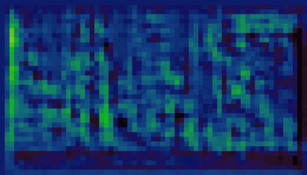
6

plus the bias,                                                             briefly describe the method here and refer the reader to
                                                                           [14], [15] for more details.
    score(p0 , . . . , pn ) =                                                Let Ri,l (x, y) = Fi0 · φ(H, (x, y, l)) be an array storing
             X n                      n
                                      X                                    the response of the i-th model filter in the l-th level
                    Fi0 · φ(H, pi ) −   di · φd (dxi , dyi ) + b, (2)      of the feature pyramid. The matching algorithm starts
             i=0                           i=1                             by computing these responses. Note that Ri,l is a cross-
where                                                                      correlation between Fi and level l of the feature pyramid.
                                                                             After computing filter responses we transform the re-
             (dxi , dyi ) = (xi , yi ) − (2(x0 , y0 ) + vi )         (3)   sponses of the part filters to allow for spatial uncertainty,
gives the displacement of the i-th part relative to its                     Di,l (x, y) = max (Ri,l (x + dx, y + dy) − di · φd (dx, dy)) .
                                                                                          dx,dy
anchor position and                                                                                                                 (8)
                 φd (dx, dy) = (dx, dy, dx , dy )    2     2
                                                                     (4)   This transformation spreads high filter scores to nearby
                                                                           locations, taking into account the deformation costs. The
are deformation features.                                                  value Di,l (x, y) is the maximum contribution of the i-th
  Note that if di = (0, 0, 1, 1) the deformation cost for                  part to the score of a root location that places the anchor
the i-th part is the squared distance between its actual                   of this part at position (x, y) in level l.
position and its anchor position relative to the root. In                    The transformed array, Di,l , can be computed in linear
general the deformation cost is an arbitrary separable                     time from the response array, Ri,l , using the generalized
quadratic function of the displacements.                                   distance transform algorithm from [14].
  The bias term is introduced in the score to make the                       The overall root scores at each level can be expressed
scores of multiple models comparable when we combine                       by the sum of the root filter response at that level, plus
them into a mixture model.                                                 shifted versions of transformed and subsampled part
  The score of a hypothesis z can be expressed in terms                    responses,
of a dot product, β · ψ(H, z), between a vector of model
parameters β and a vector ψ(H, z),                                           score(x0 , y0 , l0 ) =
                                                                                                        n
                                                                                                        X
                 β = (F00 , . . . , Fn0 , d1 , . . . , dn , b).      (5)           R0,l0 (x0 , y0 ) +         Di,l0 −λ (2(x0 , y0 ) + vi ) + b. (9)
       ψ(H, z) = (φ(H, p0 ), . . . φ(H, pn ),                                                           i=1
                                                                     (6)   Recall that λ is the number of levels we need to go down
                   −φd (dx1 , dy1 ), . . . , −φd (dxn , dyn ), 1).
                                                                           in the feature pyramid to get to a feature map that was
This illustrates a connection between our models and                       computed at exactly twice the resolution of another one.
linear classifiers. We use this relationship for learning                     Figure 4 illustrates the matching process.
the model parameters with the latent SVM framework.                           To understand equation (9) note that for a fixed root
                                                                           location we can independently pick the best location for
3.2    Matching                                                            each part because there are no interactions among parts
                                                                           in the score of a hypothesis. The transformed arrays Di,l
To detect objects in an image we compute an overall                        give the contribution of the i-th part to the overall root
score for each root location according to the best possible                score, as a function of the anchor position for the part. So
placement of the parts,                                                    we obtain the total score of a root position at level l by
             score(p0 ) = max score(p0 , . . . , pn ).               (7)   adding up the root filter response and the contributions
                              p1 ,...,pn                                   from each part, which are precomputed in Di,l−λ .
High-scoring root locations define detections while the                       In addition to computing Di,l the algorithm from [14]
locations of the parts that yield a high-scoring root                      can also compute optimal displacements for a part as a
location define a full object hypothesis.                                  function of its anchor position,
  By defining an overall score for each root location we                   Pi,l (x, y) = argmax (Ri,l (x + dx, y + dy) − di · φd (dx, dy)) .
can detect multiple instances of an object (we assume                                     dx,dy
there is at most one instance per root location). This                                                                              (10)
approach is related to sliding-window detectors because                    After finding a root location (x0 , y0 , l0 ) with high score
we can think of score(p0 ) as a score for the detection                    we can find the corresponding part locations by looking
window specified by the root filter.                                       up the optimal displacements in Pi,l0 −λ (2(x0 , y0 ) + vi ).
  We use dynamic programming and generalized dis-
tance transforms (min-convolutions) [14], [15] to com-                     3.3   Mixture Models
pute the best locations for the parts as a function of                     A mixture model with m components is defined by a
the root location. The resulting method is very efficient,                 m-tuple, M = (M1 , . . . , Mm ), where Mc is the model for
taking O(nk) time once filter responses are computed,                      the c-th component.
where n is the number of parts in the model and k is                         An object hypothesis for a mixture model specifies a
the total number of locations in the feature pyramid. We                   mixture component, 1 ≤ c ≤ m, and a location for each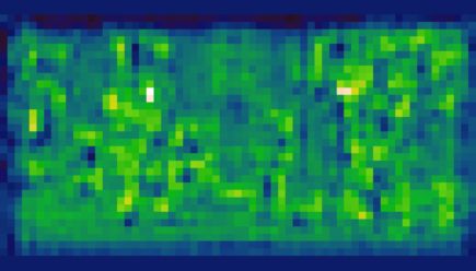
7

                                                                                    model
      feature map                                 feature map at twice the resolution

                                                          x                   ...                  x
                   x

                                                                              ...
                                                              response of part filters

    response of root filter

                                                                              ...
                                                               transformed responses

                                                           +

              color encoding of filter
                 response values

                                                                                              combined score of
           low value                  high value                                                root locations

Fig. 4. The matching process at one scale. Responses from the root and part filters are computed a different
resolutions in the feature pyramid. The transformed responses are combined to yield a final score for each root
location. We show the responses and transformed responses for the “head” and “right shoulder” parts. Note how the
“head” filter is more discriminative. The combined scores clearly show two good hypothesis for the object at this scale.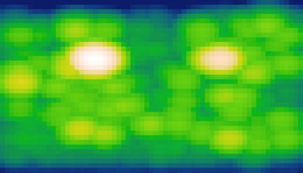
8

filter of Mc , z = (c, p0 , . . . , pnc ). Here nc is the number      convex in β and thus the hinge loss, max(0, 1 − yi fβ (xi )),
of parts in Mc . The score of this hypothesis is the score            is convex in β when yi = −1. That is, the loss function is
of the hypothesis z 0 = (p0 , . . . , pnc ) for the c-th model        convex in β for negative examples. We call this property
component.                                                            of the loss function semi-convexity.
   As in the case of a single component model the score                  In a general latent SVM the hinge loss is not convex for
of a hypothesis for a mixture model can be expressed                  a positive example because it is the maximum of a con-
by a dot product between a vector of model parameters                 vex function (zero) and a concave function (1−yi fβ (xi )).
β and a vector ψ(H, z). For a mixture model the vector                   Now consider a latent SVM where there is a single
β is the concatenation of the model parameter vectors                 possible latent value for each positive example. In this
for each component. The vector ψ(H, z) is sparse, with                case fβ (xi ) is linear for a positive example and the loss
non-zero entries defined by ψ(H, z 0 ) in a single interval           due to each positive is convex. Combined with the semi-
matching the interval of βc in β,                                     convexity property, (14) becomes convex.
                        β = (β1 , . . . , βm ).                (11)
                                             0
           ψ(H, z) = (0, . . . , 0, ψ(H, z ), 0, . . . , 0).   (12)   4.2   Optimization
                                                                      Let Zp specify a latent value for each positive example
With this construction β · ψ(H, z) = βc · ψ(H, z 0 ).
                                                                      in a training set D. We can define an auxiliary objective
   To detect objects using a mixture model we use the
                                                                      function LD (β, Zp ) = LD(Zp ) (β), where D(Zp ) is derived
matching algorithm described above to find root loca-
                                                                      from D by restricting the latent values for the positive
tions that yield high scoring hypotheses independently
                                                                      examples according to Zp . That is, for a positive example
for each component.
                                                                      we set Z(xi ) = {zi } where zi is the latent value specified
                                                                      for xi by Zp . Note that
4     L ATENT SVM
Consider a classifier that scores an example x with a                                  LD (β) = min LD (β, Zp ).              (15)
                                                                                                  Zp
function of the form,
                                                                      In particular LD (β) ≤ LD (β, Zp ). The auxiliary objective
                   fβ (x) = max β · Φ(x, z).                   (13)   function bounds the LSVM objective. This justifies train-
                             z∈Z(x)
                                                                      ing a latent SVM by minimizing LD (β, Zp ).
Here β is a vector of model parameters and z are latent                  In practice we minimize LD (β, Zp ) using a “coordinate
values. The set Z(x) defines the possible latent values               descent” approach:
for an example x. A binary label for x can be obtained
                                                                         1) Relabel positive examples: Optimize LD (β, Zp ) over
by thresholding its score.
                                                                            Zp by selecting the highest scoring latent value for
  In analogy to classical SVMs we train β from labeled
                                                                            each positive example,
examples D = (hx1 , y1 i, . . . , hxn , yn i), where yi ∈ {−1, 1},
                                                                            zi = argmaxz∈Z(xi ) β · Φ(xi , z).
by minimizing the objective function,
                                                                         2) Optimize beta: Optimize LD (β, Zp ) over β by solv-
                                n
                 1            X                                             ing the convex optimization problem defined by
      LD (β) =     ||β||2 + C     max(0, 1 − yi fβ (xi )),     (14)
                 2                                                          LD(Zp ) (β).
                              i=1
                                                                      Both steps always improve or maintain the value of
where max(0, 1 − yi fβ (xi )) is the standard hinge loss              LD (β, Zp ). After convergence we have a relatively strong
and the constant C controls the relative weight of the                local optimum in the sense that step 1 searches over
regularization term.                                                  an exponentially-large space of latent values for positive
  Note that if there is a single possible latent value for            examples while step 2 searches over all possible models,
each example (|Z(xi )| = 1) then fβ is linear in β, and we            implicitly considering the exponentially-large space of
obtain linear SVMs as a special case of latent SVMs.                  latent values for all negative examples.
                                                                         We note, however, that careful initialization of β may
4.1    Semi-convexity                                                 be necessary because otherwise we may select unreason-
A latent SVM leads to a non-convex optimization prob-                 able latent values for the positive examples in step 1, and
lem. However, a latent SVM is semi-convex in the sense                this could lead to a bad model.
described below, and the training problem becomes con-                   The semi-convexity property is important because it
vex once latent information is specified for the positive             leads to a convex optimization problem in step 2, even
training examples.                                                    though the latent values for the negative examples are
   Recall that the maximum of a set of convex functions               not fixed. A similar procedure that fixes latent values
is convex. In a linear SVM we have that fβ (x) = β · Φ(x)             for all examples in each round would likely fail to yield
is linear in β. In this case the hinge loss is convex for             good results. Suppose we let Z specify latent values for
each example because it is always the maximum of two                  all examples in D. Since LD (β) effectively maximizes
convex functions.                                                     over negative latent values, LD (β) could be much larger
   Note that fβ (x) as defined in (13) is a maximum of                than LD (β, Z), and we should not expect that minimiz-
functions each of which is linear in β. Hence fβ (x) is               ing LD (β, Z) would lead to a good model.
9
4.3 Stochastic gradient descent problems using a relatively small number of hard exam-
Step 2 (Optimize Beta) of the coordinate descent method ples and converges to the exact solution of the training
can be solved via quadratic programming [3]. It can problem defined by a large training set. This requires a
also be solved via stochastic gradient descent. Here we margin-sensitive definition of hard examples.
describe a gradient descent approach for optimizing β We define hard and easy instances of a training set D
over an arbitrary training set D. In practice we use a relative to β as follows,
modified version of this procedure that works with a
H(β, D) = {hx, yi ∈ D | yfβ (x) < 1}. (18)
cache of feature vectors for D(Zp ) (see Section 4.5).
Let zi (β) = argmaxz∈Z(xi ) β · Φ(xi , z). E(β, D) = {hx, yi ∈ D | yfβ (x) > 1}. (19)
Then fβ (xi ) = β · Φ(xi , zi (β)).
We can compute a sub-gradient of the LSVM objective That is, H(β, D) are the examples in D that are incor-
function as follows, rectly classified or inside the margin of the classifier
n
X defined by β. Similarly E(β, D) are the examples in
∇LD (β) = β + C h(β, xi , yi ) (16) D that are correctly classified and outside the margin.
i=1 Examples on the margin are neither hard nor easy.
0 if yi fβ (xi ) ≥ 1 Let β ∗ (D) = argminβ LD (β).
h(β, xi , yi ) =
−yi Φ(xi , zi (β)) otherwise
(17) Since LD is strictly convex β ∗ (D) is unique.
Given a large training set D we would like to find a
In stochastic gradient descent we approximate ∇LD small set of examples C ⊆ D such that β ∗ (C) = β ∗ (D).
using a subset of the examples and take a step in Our method starts with an initial “cache” of examples
Pn Using a single example, hxi , yi i,
its negative direction. and alternates between training a model and updating
we approximate i=1 h(β, xi , yi ) with nh(β, xi , yi ). The the cache. In each iteration we remove easy examples
resulting algorithm repeatedly updates β as follows: from the cache and add new hard examples. A special
1) Let αt be the learning rate for iteration t. case involves keeping all positive examples in the cache
2) Let i be a random example. and data-mining over negatives.
3) Let zi = argmaxz∈Z(xi ) β · Φ(xi , z). Let C1 ⊆ D be an initial cache of examples. The
4) If yi fβ (xi ) = yi (β · Φ(xi , zi )) ≥ 1 set β := β − αt β. algorithm repeatedly trains a model and updates the
5) Else set β := β − αt (β − Cnyi Φ(xi , zi )). cache as follows:
As in gradient descent methods for linear SVMs we 1) Let βt := β ∗ (Ct ) (train a model using Ct ).
obtain a procedure that is quite similar to the perceptron 2) If H(βt , D) ⊆ Ct stop and return βt .
algorithm. If fβ correctly classifies the random example 3) Let Ct0 := Ct \X for any X such that X ⊆ E(βt , Ct )
xi (beyond the margin) we simply shrink β. Otherwise (shrink the cache).
we shrink β and add a scalar multiple of Φ(xi , zi ) to it. 4) Let Ct+1 := Ct0 ∪ X for any X such that X ⊆ D and
For linear SVMs a learning rate αt = 1/t has been X ∩ H(βt , D)\Ct 6= ∅ (grow the cache).
shown to work well [37]. However, the time for con- In step 3 we shrink the cache by removing examples
vergence depends on the number of training examples, from Ct that are outside the margin defined by βt . In
which for us can be very large. In particular, if there step 4 we grow the cache by adding examples from
are many “easy” examples, step 2 will often pick one of D, including at least one new example that is inside
these and we do not make much progress. the margin defined by βt . Such example must exist
otherwise we would have returned in step 2.
4.4 Data-mining hard examples, SVM version The following theorem shows that when we stop we
When training a model for object detection we often have found β ∗ (D).
have a very large number of negative examples (a single Theorem 1: Let C ⊆ D and β = β ∗ (C). If H(β, D) ⊆ C
image can yield 105 examples for a scanning window then β = β ∗ (D).
classifier). This can make it infeasible to consider all Proof: C ⊆ D implies LD (β ∗ (D)) ≥ LC (β ∗ (C)) =
negative examples simultaneously. Instead, it is common LC (β). Since H(β, D) ⊆ C all examples in D\C have
to construct training data consisting of the positive in- zero loss on β. This implies LC (β) = LD (β). We conclude
stances and “hard negative” instances. LD (β ∗ (D)) ≥ LD (β), and because LD has a unique
Bootstrapping methods train a model with an initial minimum β = β ∗ (D).
subset of negative examples, and then collect negative The next result shows the algorithm will stop after a
examples that are incorrectly classified by this initial finite number of iterations. Intuitively this follows from
model to form a set of hard negatives. A new model is the fact that LCt (β ∗ (Ct )) grows in each iteration, but it
trained with the hard negative examples and the process is bounded by LD (β ∗ (D)).
may be repeated a few times. Theorem 2: The data-mining algorithm terminates.
Here we describe a data-mining algorithm motivated Proof: When we shrink the cache Ct0 contains all
by the bootstrapping idea for training a classical (non- examples from Ct with non-zero loss in a ball around
latent) SVM. The method solves a sequence of training βt . This implies LCt0 is identical to LCt in a ball around10
βt , and since βt is a minimum of LCt it also must be a We define the hard feature vectors of a training set D
minimum of LCt0 . Thus LCt0 (β ∗ (Ct0 )) = LCt (β ∗ (Ct )). relative to β as,
When we grow the cache Ct+1 \Ct0 contains at least one
example hx, yi with non-zero loss at βt . Since Ct0 ⊆ Ct+1 H(β, D) = {(i, Φ(xi , zi )) |
we have LCt+1 (β) ≥ LCt0 (β) for all β. If β ∗ (Ct+1 ) 6= zi = argmax β · Φ(xi , z) and yi (β · Φ(xi , zi )) < 1}. (21)
β ∗ (Ct0 ) then LCt+1 (β ∗ (Ct+1 )) > LCt0 (β ∗ (Ct0 )) because LCt0 z∈Z(xi )
has a unique minimum. If β ∗ (Ct+1 ) = β ∗ (Ct0 ) then That is, H(β, D) are pairs (i, v) where v is the highest
LCt+1 (β ∗ (Ct+1 )) > LCt0 (β ∗ (Ct0 )) due to hx, yi. scoring feature vector from an example xi that is inside
We conclude LCt+1 (β ∗ (Ct+1 )) > LCt (β ∗ (Ct )). Since the margin of the classifier defined by β.
there are finitely many caches the loss in the cache can We define the easy feature vectors in a cache F as
only grow a finite number of times.
E(β, F ) = {(i, v) ∈ F | yi (β · v) > 1} (22)
These are the feature vectors from F that are outside the
4.5 Data-mining hard examples, LSVM version
margin defined by β.
Now we describe a data-mining algorithm for training a Note that if yi (β · v) ≤ 1 then (i, v) is not considered
latent SVM when the latent values for the positive examples easy even if there is another feature vector for the i-th
are fixed. That is, we are optimizing LD(Zp ) (β), and not example in the cache with higher score than v under β.
LD (β). As discussed above this restriction ensures the Now we describe the data-mining algorithm for com-
optimization problem is convex. puting β ∗ (D(Zp )).
For a latent SVM instead of keeping a cache of exam- The algorithm works with a cache of feature vectors
ples x, we keep a cache of (x, z) pairs where z ∈ Z(x). for D(Zp ). It alternates between training a model and
This makes it possible to avoid doing inference over all updating the cache.
of Z(x) in the inner loop of an optimization algorithm Let F1 be an initial cache of feature vectors. Now
such as gradient descent. Moreover, in practice we can consider the following iterative algorithm:
keep a cache of feature vectors, Φ(x, z), instead of (x, z) 1) Let βt := β ∗ (Ft ) (train a model).
pairs. This representation is simpler (its application in- 2) If H(β, D(Zp )) ⊆ Ft stop and return βt .
dependent) and can be much more compact. 3) Let Ft0 := Ft \X for any X such that X ⊆ E(βt , Ft )
A feature vector cache F is a set of pairs (i, v) where (shrink the cache).
1 ≤ i ≤ n is the index of an example and v = Φ(xi , z) for 4) Let Ft+1 := Ft0 ∪ X for any X such that
some z ∈ Z(xi ). Note that we may have several pairs X ∩ H(βt , D(Zp ))\Ft 6= ∅ (grow the cache).
(i, v) ∈ F for each example xi . If the training set has Sstep 3 shrinks the cache by removing easy feature
fixed labels for positive examples this may still be true vetors. Step 4 grows the cache by adding “new” feature
for the negative examples. vectors, including at least one from H(βt , D(Zp )). Note
Let I(F ) be the examples indexed by F . The feature that over time we will accumulate multiple feature vec-
vectors in F define an objective function for β, where we tors from the same negative example in the cache.
only consider examples indexed by I(F ), and for each We can show this algorithm will eventually stop and
example we only consider feature vectors in the cache, return β ∗ (D(Zp )). This follows from arguments analo-
gous to the ones used in Section 4.4.
1 X
LF (β) = ||β||2 +C max(0, 1−yi ( max β·v)). (20)
2 (i,v)∈F
i∈I(F )
5 T RAINING M ODELS
We can optimize LF via gradient descent by modi- Now we consider the problem of training models from
fying the method in Section 4.3. Let V (i) be the set of images labeled with bounding boxes around objects of
feature vectors v such that (i, v) ∈ F . Then each gradient interest. This is the type of data available in the PASCAL
descent iteration simplifies to: datasets. Each dataset contains thousands of images and
each image has annotations specifying a bounding box
1) Let αt be the learning rate for iteration t.
and a class label for each target object present in the
2) Let i ∈ I(F ) be a random example indexed by F .
image. Note that this is a weakly labeled setting since
3) Let vi = argmaxv∈V (i) β · v.
the bounding boxes do not specify component labels or
4) If yi (β · vi ) ≥ 1 set β = β − αt β.
part locations.
5) Else set β = β − αt (β − Cnyi vi ).
We describe a procedure for initializing the structure
Now the size of I(F ) controls the number of iterations of a mixture model and learning all parameters. Pa-
necessary for convergence, while the size of V (i) controls rameter learning is done by constructing a latent SVM
the time it takes to execute step 3. In step 5 n = |I(F )|. training problem. We train the latent SVM using the
Let β ∗ (F ) = argminβ LF (β). coordinate descent approach described in Section 4.2
We would like to find a small cache for D(Zp ) with together with the data-mining and gradient descent
β ∗ (F ) = β ∗ (D(Zp )). algorithms that work with a cache of feature vectors11
from Section 4.5. Since the coordinate descent method is easy feature vectors. During data-mining we grow the
susceptible to local minima we must take care to ensure cache by iterating over the images in N sequentially,
a good initialization of the model. until we reach a memory limit.
Data:
5.1 Learning parameters
Positive examples P = {(I1 , B1 ), . . . , (In , Bn )}
Let c be an object class. We assume the training examples Negative images N = {J1 , . . . , Jm }
for c are given by positive bounding boxes P and a set Initial model β
of background images N . P is a set of pairs (I, B) where
Result: New model β
I is an image and B is a bounding box for an object of
class c in I. 1 Fn := ∅
Let M be a (mixture) model with fixed structure. Recall 2 for relabel := 1 to num-relabel do
that the parameters for a model are defined by a vector 3 Fp := ∅
β. To learn β we define a latent SVM training problem 4 for i := 1 to n do
with an implicitly defined training set D, with positive 5 Add detect-best(β,Ii ,Bi ) to Fp
examples from P , and negative examples from N . 6 end
Each example hx, yi ∈ D has an associated image and 7 for datamine := 1 to num-datamine do
feature pyramid H(x). Latent values z ∈ Z(x) specify an 8 for j := 1 to m do
instantiation of M in the feature pyramid H(x). 9 if |Fn | ≥ memory-limit then break
Now define Φ(x, z) = ψ(H(x), z). Then β · Φ(x, z) is 10 Add detect-all(β,Jj ,−(1 + δ)) to Fn
exactly the score of the hypothesis z for M on H(x). 11 end
A positive bounding box (I, B) ∈ P specifies that the 12 β :=gradient-descent(Fp ∪ Fn )
object detector should “fire” in a location defined by B. 13 Remove (i, v) with β · v < −(1 + δ) from Fn
This means the overall score (7) of a root location defined 14 end
by B should be high. 15 end
For each (I, B) ∈ P we define a positive example x Procedure Train
for the LSVM training problem. We define Z(x) so the
detection window of a root filter specified by a hypoth- The function detect-best(β, I, B) finds the highest
esis z ∈ Z(x) overlaps with B by at least 50%. There scoring object hypothesis with a root filter that signifi-
are usually many root locations, including at different cantly overlaps B in I. The function detect-all(β, I, t)
scales, that define detection windows with 50% overlap. computes the best object hypothesis for each root lo-
We have found that treating the root location as a latent cation and selects the ones that score above t. Both of
variable is helpful to compensate for noisy bounding box these functions can be implemented using the matching
labels in P . A similar idea was used in [40]. procedure in Section 3.2.
Now consider a background image I ∈ N . We do not The function gradient-descent(F ) trains β using
want the object detector to “fire” in any location of the feature vectors in the cache as described in Section 4.5.
feature pyramid for I. This means the overall score (7) of In practice we modified the algorithm to constrain the
every root location should be low. Let G be a dense set of coefficients of the quadratic terms in the deformation
locations in the feature pyramid. We define a different models to be above 0.01. This ensures the deformation
negative example x for each location (i, j, l) ∈ G. We costs are convex, and not “too flat”. We also constrain
define Z(x) so the level of the root filter specified by the model to be symmetric along the vertical axis. Filters
z ∈ Z(x) is l, and the center of its detection window is that are positioned along the center vertical axis of the
(i, j). Note that there is a very large number of negative model are constrained to be self-symmetric. Part filters
examples obtained from each image. This is consistent that are off-center have a symmetric part on the other
with the requirement that a scanning window classifier side of the model. This effectively reduces the number
should have low false positive rate. of parameters to be learned in half.
The procedure Train is outlined below. The outer-
most loop implements a fixed number of iterations of 5.2 Initialization
coordinate descent on LD (β, Zp ). Lines 3-6 implement The LSVM coordinate descent algorithm is susceptible to
the Relabel positives step. The resulting feature vectors, local minima and thus sensitive to initialization. This is
one per positive example, are stored in Fp . Lines 7-14 a common limitation of other methods that use latent
implement the Optimize beta step. Since the number of information as well. We initialize and train mixture
negative examples implicitly defined by N is very large models in three phases as follows.
we use the LSVM data-mining algorithm. We iterate Phase 1. Initializing Root Filters: For training a
data-mining a fixed number of times rather than until mixture model with m components we sort the bounding
convergence for practical reasons. At each iteration we boxes in P by their aspect ratio and split them into m
collect hard negative examples in Fn , train a new model groups of equal size P1 , . . . , Pm . Aspect ratio is used as a
using gradient descent, and then shrink Fn by removing simple indicator of extreme intraclass variation. We train12
m different root filters F1 , . . . , Fm , one for each group of augmenting this low-dimensional feature set to include
positive bounding boxes. both contrast sensitive and contrast insensitive features,
To define the dimensions of Fi we select the mean leading to a 31-dimensional feature vector, improves
aspect ratio of the boxes in Pi and the largest area not performance for most classes of the PASCAL datasets.
larger than 80% of the boxes. This ensures that for most
pairs (I, B) ∈ Pi we can place Fi in the feature pyramid
6.1 HOG Features
of I so it significantly overlaps with B.
We train Fi using a standard SVM, with no latent 6.1.1 Pixel-Level Feature Maps
information, as in [10]. For (I, B) ∈ Pi we warp the Let θ(x, y) and r(x, y) be the orientation and magnitude
image region under B so its feature map has the same of the intensity gradient at a pixel (x, y) in an image.
dimensions as Fi . This leads to a positive example. We As in [10], we compute gradients using finite difference
select random subwindows of appropriate dimension filters, [−1, 0, +1] and its transpose. For color images we
from images in N to define negative examples. Fig- use the color channel with the largest gradient magni-
ures 5(a) and 5(b) show the result of this phase when tude to define θ and r at each pixel.
training a two component car model. The gradient orientation at each pixel is discretized
Phase 2. Merging Components: We combine the into one of p values using either a contrast sensitive (B1 ),
initial root filters into a mixture model with no parts or insensitive (B2 ), definition,
and retrain the parameters of the combined model us-
pθ(x, y)
ing Train on the full (unsplit and without warping) B1 (x, y) = round mod p (23)
data sets P and N . In this case the component label 2π
and root location are the only latent variables for each pθ(x, y)
B2 (x, y) = round mod p (24)
example. The coordinate descent training algorithm can π
be thought of as a discriminative clustering method that Below we use B to denote either B1 or B2 .
alternates between assigning cluster (mixture) labels for We define a pixel-level feature map that specifies a
each positive example and estimating cluster “means” sparse histogram of gradient magnitudes at each pixel.
(root filters). Let b ∈ {0, . . . , p − 1} range over orientation bins. The
Phase 3. Initializing Part Filters: We initialize the feature vector at (x, y) is
parts of each component using a simple heuristic. We
fix the number of parts at six per component, and using r(x, y) if b = B(x, y)
F (x, y)b = (25)
a small pool of rectangular part shapes we greedily place 0 otherwise
parts to cover high-energy regions of the root filter.2 A
We can think of F as an oriented edge map with p
part is either anchored along the central vertical axis of
orientation channels. For each pixel we select a channel
the root filter, or it is off-center and has a symmetric part
by discretizing the gradient orientation. The gradient
on the other side of the root filter. Once a part is placed,
magnitude can be seen as a measure of edge strength.
the energy of the covered portion of the root filter is set
to zero, and we look for the next highest-energy region,
6.1.2 Spatial Aggregation
until six parts are chosen.
The part filters are initialized by interpolating the root Let F be a pixel-level feature map for a w × h image.
filter to twice the spatial resolution. The deformation pa- Let k > 0 be a parameter specifying the side length
rameters for each part are initialized to di = (0, 0, .1, .1). of a square image region. We define a dense grid of
This pushes part locations to be fairly close to their rectangular “cells” and aggregate pixel-level features to
anchor position. Figure 5(c) shows the results of this obtain a cell-based feature map C, with feature vectors
phase when training a two component car model. The C(i, j) for 0 ≤ i ≤ b(w − 1)/kc and 0 ≤ j ≤ b(h − 1)/kc.
resulting model serves as the initial model for the last This aggregation provides some invariance to small de-
round of parameter learning. The final car model is formations and reduces the size of a feature map.
shown in Figure 9. The simplest approach for aggregating features is to
map each pixel (x, y) into a cell (bx/kc, by/kc) and define
the feature vector at a cell to be the sum (or average) of
6 F EATURES
the pixel-level features in that cell.
Here we describe the 36-dimensional histogram of ori- Rather than mapping each pixel to a unique cell we
ented gradients (HOG) features from [10] and introduce follow [10] and use a “soft binning” approach where
an alternative 13-dimensional feature set that captures each pixel contributes to the feature vectors in the four
essentially the same information.3 We have found that cells around it using bilinear interpolation.
2. The “energy” of a region is defined by the norm of the positive
weights in a subwindow. 6.1.3 Normalization and Truncation
3. There are some small differences between the 36-dimensional Gradients are invariant to changes in bias. Invariance
features defined here and the ones in [10], but we have found that
these differences did not have any significant effect on the performance to gain can be achieved via normalization. Dalal and
of our system. Triggs [10] used four different normalization factors for13
(a) (c)
(b)
Fig. 5. (a) and (b) are the initial root filters for a car model (the result of Phase 1 of the initialization process). (c) is the
initial part-based model for a car (the result of Phase 3 of the initialization process).
the feature vector C(i, j). We can write these factors as Recall that a 36-dimensional HOG feature is defined
Nδ,γ (i, j) with δ, γ ∈ {−1, 1}, using 4 different normalizations of a 9 dimensional his-
togram over orientations. Thus a 36-dimensional HOG
Nδ,γ (i, j) = (||C(i, j)||2 + ||C(i + δ, j)||2 + feature is naturally viewed as a 4 × 9 matrix. The top
1
||C(i, j + γ)||2 + ||C(i + δ, j + γ)||2 ) 2 . (26) eigenvectors in Figure 6 have a very special structure:
they are each (approximately) constant along each row
Each factor measures the “gradient energy” in a square or column of their matrix representation. Thus the top
block of four cells containing (i, j). eigenvectors lie (approximately) in a linear subspace
Let Tα (v) denote the component-wise truncation of a defined by sparse vectors that have ones along a single
vector v by α (the i-th entry in Tα (v) is the minimum row or column of their matrix representation.
of the i-th entry of v and α). The HOG feature map is Let V = {u1 , . . . , u9 } ∪ {v1 , . . . , v4 } with
obtained by concatenating the result of normalizing the
cell-based feature map C with respect to each normal- 1 if j = k
uk (i, j) = (28)
ization factor followed by truncation, 0 otherwise
1 if i = k
Tα (C(i, j)/N−1,−1 (i, j)) vk (i, j) = (29)
Tα (C(i, j)/N+1,−1 (i, j)) 0 otherwise
H(i, j) =
Tα (C(i, j)/N+1,+1 (i, j)) (27)
We can define a 13-dimensional feature by taking the
Tα (C(i, j)/N−1,+1 (i, j))
dot product of a 36-dimensional HOG feature with each
Commonly used HOG features are defined using p = uk and vk . Projection into each uk is computed by sum-
9 contrast insensitive gradient orientations (discretized ming over the 4 normalizations for a fixed orientation.
with B2 ), a cell size of k = 8 and truncation α = 0.2. Projection into each vk is computed by summing over 9
This leads to a 36-dimensional feature vector. We used orientations for a fixed normalization.4
these parameters in the analysis described below. As in the case of 11-dimensional PCA features we
obtain the same performance using the 36-dimensional
6.2 PCA and Analytic Dimensionality Reduction HOG features or the 13-dimensional features defined
We collected a large number of 36-dimensional HOG by V . However, the computation of the 13-dimensional
features from different resolutions of a large number features is much less costly than performing projections
of images and performed PCA on these vectors. The to the top eigenvectors obtained via PCA since the uk
principal components are shown in Figure 6. The results and vk are sparse. Moreover, the 13-dimensional features
lead to a number of interesting discoveries. have a simple interpretation as 9 orientation features
The eigenvalues indicate that the linear subspace and 4 features that reflect the overall gradient energy
spanned by the top 11 eigenvectors captures essentially in different areas around a cell.
all the information in a HOG feature. In fact we obtain We can also define low-dimensional features that are
the same detection performance in all categories of the contrast sensitive. We have found that performance on
PASCAL 2007 dataset using the original 36-dimensional some object categories improves using contrast sensitive
features or 11-dimensional features defined by projec- features, while some categories benefit from contrast
tion to the top eigenvectors. Using lower dimensional insensitive features. Thus in practice we use feature vec-
features leads to models with fewer parameters and tors that include both contrast sensitive and insensitive
speeds up the detection and learning algorithms. We information.
note however that some of the gain is lost because we
4. The 13-dimensional feature is not a linear projection of the 36-
need to perform a relatively costly projection step when dimensional feature into V because the uk and vk are not orthogonal.
computing feature pyramids. In fact the linear subspace spanned by V has dimension 12.You can also read


