Himawari-8-derived diurnal variations in ground-level PM2.5 pollution across China using the fast space-time Light Gradient Boosting Machine ...
←
→
Page content transcription
If your browser does not render page correctly, please read the page content below
Atmos. Chem. Phys., 21, 7863–7880, 2021
https://doi.org/10.5194/acp-21-7863-2021
© Author(s) 2021. This work is distributed under
the Creative Commons Attribution 4.0 License.

Himawari-8-derived diurnal variations in ground-level PM2.5
pollution across China using the fast space-time Light Gradient
Boosting Machine (LightGBM)
Jing Wei1,2,3 , Zhanqing Li2 , Rachel T. Pinker2 , Jun Wang3 , Lin Sun4 , Wenhao Xue1 , Runze Li1 , and Maureen Cribb2
1 StateKey Laboratory of Remote Sensing Science, College of Global Change and Earth System Science,
Beijing Normal University, Beijing, China
2 Earth System Science Interdisciplinary Center, Department of Atmospheric and Oceanic Science,

University of Maryland, College Park, MD, USA
3 Department of Chemical and Biochemical Engineering, Iowa Technology Institute, Center for Global and Regional

Environmental Research, The University of Iowa, Iowa City, IA, USA
4 College of Geodesy and Geomatics, Shandong University of Science and Technology, Qingdao, China

Correspondence: Jing Wei (weijing_rs@163.com) and Zhanqing Li (zhanqing@umd.edu)

Received: 16 December 2020 – Discussion started: 6 January 2021
Revised: 28 March 2021 – Accepted: 18 April 2021 – Published: 25 May 2021

Abstract. Fine particulate matter with a diameter of less       well the PM2.5 diurnal variations showing that pollution in-
than 2.5 µm (PM2.5 ) has been used as an important atmo-        creases gradually in the morning, reaching a peak at about
spheric environmental parameter mainly because of its im-       10:00 LT (GMT+8), then decreases steadily until sunset. The
pact on human health. PM2.5 is affected by both natural         proposed approach outperforms most traditional statistical
and anthropogenic factors that usually have strong diur-        regression and tree-based machine-learning models with a
nal variations. Such information helps toward understanding     much lower computational burden in terms of speed and
the causes of air pollution, as well as our adaptation to it.   memory, making it most suitable for routine pollution moni-
Most existing PM2.5 products have been derived from polar-      toring.
orbiting satellites. This study exploits the use of the next-
generation geostationary meteorological satellite Himawari-
8/AHI (Advanced Himawari Imager) to document the diur-
nal variation in PM2.5 . Given the huge volume of satellite     1   Introduction
data, based on the idea of gradient boosting, a highly ef-
ficient tree-based Light Gradient Boosting Machine (Light-      China has faced severe environmental problems during the
GBM) method by involving the spatiotemporal character-          last 2 decades, especially air pollution (An et al., 2019; Chan
istics of air pollution, namely the space-time LightGBM         and Yao, 2008; Z. Li et al., 2017; Q. Zhang et al., 2019;
(STLG) model, is developed. An hourly PM2.5 dataset for         Wei et al., 2021a). The sources of air pollution are numer-
China (i.e., ChinaHighPM2.5 ) at a 5 km spatial resolution      ous, coming from both natural changes (e.g., forest fires,
is derived based on Himawari-8/AHI aerosol products with        biomass burning) and human activities (e.g., industrial pro-
additional environmental variables. Hourly PM2.5 estimates      duction, transportation) (Huang et al., 2014; Sun et al., 2004;
(number of data samples = 1 415 188) are well correlated        Wei et al., 2019a, b, 2021b). Particulate matter with a di-
with ground measurements in China (cross-validation coef-       ameter of less than 2.5 µm (PM2.5 ) has a greater impact on
ficient of determination, CV-R 2 = 0.85), with a root-mean-     the atmospheric environment and climate change than other
square error (RMSE) and mean absolute error (MAE) of            air pollutants (e.g., PM10 , nitrogen dioxide, NO2 , and sulfur
13.62 and 8.49 µg m−3 , respectively. Our model captures        dioxide, SO2 ) (Jacob and Winner, 2009; Z. Li et al., 2017,
                                                                2019; Ramanathan and Feng, 2009). Moreover, they can

Published by Copernicus Publications on behalf of the European Geosciences Union.
7864                            J. Wei et al.: Hourly PM2.5 mapping across China using the space-time LightGBM model

cause great harm to human health due to their smaller par-         ies (Chen et al., 2019; Liu et al., 2019; Sun et al., 2019; Wang
ticle size (Delfino et al., 2005; Kampa and Castanas, 2008;        et al., 2017; T. Zhang et al., 2019), resulting in relatively low
Kim et al., 2015; Lelieveld et al., 2015). China has estab-        accuracies.
lished and operates multiple ground-based observation net-            Focusing on the above issues, we have developed a new,
works to monitor air pollution in real time across mainland        highly efficient, and precise method for improving ground-
China, including information about PM2.5 pollution.                level PM2.5 estimates by incorporating spatial and tempo-
   For near-surface concentrations, the networks provide           ral information into the tree-based Light Gradient Boosting
high-quality PM2.5 measurements every hour (even every             Machine (LightGBM) model. This new model is called the
few minutes) but with non-uniform coverage. In recent years,       space-time LightGBM (STLG) model, and it has been used
an increased effort has been made in estimating PM2.5              to generate a high-quality, high-temporal-resolution (hourly)
with products generated from multiple instruments on sun-          PM2.5 dataset over eastern China (at a spatial resolution of
synchronous satellites, e.g., the Multi-angle Imaging Spec-        5 km) from the Himawari-8/AHI hourly AOD product. Sec-
troRadiometer (MISR) (Liu et al., 2005; van Donkelaar et al.,      tion 2 provides details about the data used and introduces
2006), the Moderate Resolution Imaging Spectroradiometer           the development of the STLG model. Section 3 validates the
(MODIS) (Liu et al., 2007; Ma et al., 2014; Wei et al., 2019a,     hourly PM2.5 estimates and shows the diurnal PM2.5 varia-
2020, 2021a), and the Visible Infrared Imaging Radiometer          tions across China. Comparisons with results from traditional
Suite (VIIRS) (Wei et al., 2021c; Wu et al., 2016; Yao et          models and from previous studies are also presented. Sec-
al., 2019). However, due to their low revisit cycles (one or       tion 4 summarizes the study.
two overpasses per day), they are unable to monitor the di-
urnal variation in pollution. Currently, most available PM2.5
datasets are at low temporal resolutions that cannot meet the      2     Materials and methods
requirements of air pollution real-time monitoring (Lennart-
son et al., 2018). For example, knowing when heavy pollu-          2.1     Data sources
tion might occur during the day, people may adjust their time
                                                                   2.1.1    PM2.5 and AOD data
outdoors doing activities accordingly. Following the launch
of the Himawari-8 Advanced Himawari Imager (Himawari-              PM2.5 hourly measurements from 1583 monitoring stations
8/AHI) on 7 October 2014 (Bessho et al., 2016; Letu et             across China for the year 2018 were collected (Fig. 1 in Wei
al., 2020), near-surface PM2.5 concentrations in the Eastern       et al., 2020). The latest Himawari-8 version 2 hourly 5 km
Hemisphere can now be estimated and used to examine their          AODs at 500 nm across mainland China for that year were
diurnal cycle.                                                     also collected. This AOD product is synthesized from level 2
   Wang et al. (2017) used the linear mixed-effect (LME)           10 min AODs generated by a newly developed Lambertian-
model, and Sun et al. (2019) applied the geographically            surface-assumed aerosol retrieval algorithm (Letu et al.,
weighted regression (GWR) and support vector regres-               2020; Yoshida et al., 2018). Himawari-8 AOD retrievals have
sion (SVR) models to estimate hourly PM2.5 concentra-              been preliminarily evaluated against in situ AOD retrievals
tions in the Beijing–Tianjin–Hebei (BTH) region from the           provided by the Aerosol Robotic Network (Giles et al., 2019)
Himawari-8 aerosol optical depth (AOD) product. T. Zhang           and the Sun–Sky Radiometer Observation Network (Li et
et al. (2019) developed an improved LME model, and Xue et          al., 2018), showing that they are consistent (R = 0.75), with
al. (2020) proposed an improved geographically and tempo-          a root-mean-square error (RMSE) and mean absolute error
rally weighted regression (IGTWR) model to derive hourly           (MAE) of 0.39 and 0.21, respectively (Wei et al., 2019c).
PM2.5 maps based on the Himawari-8 AOD product over                Here, only low-uncertainty AOD retrievals (500 nm) were se-
central and eastern China. In addition to traditional statis-      lected for estimating PM2.5 concentrations.
tical regression models, several artificial intelligence mod-
els, including the random forest (RF), the gradient boost-         2.1.2    Meteorological conditions
ing decision tree (GBDT), the eXtreme Gradient Boosting
(XGBoost), and the deep neural network (DNN), have been            PM2.5 can be significantly affected by meteorological con-
recently successfully adopted to obtain ground-level PM2.5         ditions (Su et al., 2018). However, most currently avail-
concentrations in local regions and in the whole of China          able reanalysis meteorological products have low tempo-
(Chen et al., 2019; Gui et al., 2020; Liu et al., 2019; Sun et     ral resolutions (∼ 3–6 h). Recently (14 June 2018), the
al., 2019; Zhang et al., 2020). Nevertheless, due to their poor    fifth-generation European Centre for Medium-range Weather
data-mining ability, traditional statistical regression methods    Forecasts (ECMWF) global atmospheric reanalysis (ERA5)
usually suffer from large uncertainties. While artificial intel-   at a horizontal resolution of 0.25◦ × 0.25◦ has been released,
ligence methods can achieve high accuracies, they are often        as well as the land version (12 July 2019) at a horizontal reso-
highly demanding on computational power and are thus often         lution of 0.1◦ × 0.1◦ , both at an hourly timescale (1979 to the
slow. Therefore, spatiotemporal variations in PM2.5 have of-       present). Here, we use seven ERA5 hourly meteorological
ten been neglected in the models developed in previous stud-       parameters, i.e., the 2 m temperature (TEM), total evapora-

Atmos. Chem. Phys., 21, 7863–7880, 2021                                              https://doi.org/10.5194/acp-21-7863-2021
J. Wei et al.: Hourly PM2.5 mapping across China using the space-time LightGBM model                                                                  7865

tion (ET), relative humidity (RH), 10 m u- and v-components         2. Gradient-based one-side sampling. Data samples are
of wind, surface pressure (SP), and boundary-layer height              first sorted in descending order according to their ab-
(BLH).                                                                 solute gradients, and the top a % of them are selected as
                                                                       a subset sample with large gradients. The b % samples
2.1.3    Human influences                                              are then randomly chosen from the remaining data as a
                                                                       subset sample with small gradients. The sampled data
Human activity is a key factor affecting PM2.5 pollution. The          with small
global annual LandScan™ product at a 1 km spatial reso-                           gradients are multiplied by a weight coeffi-
lution for the year 2018 was selected to obtain the popula-            cient 1−a b   . Consequently, a new classifier is learned
tion distribution (POP) (Dobson et al., 2000). Monthly an-             and established using the above-sampled data until con-
thropogenic source emission data from the Multi-resolution             vergence.
Emission Inventory for China (MEIC) (M. Li et al., 2017;
Zheng et al., 2018) were also employed. This dataset is gen-        3. Exclusive feature bundling. A graph with weighted
erated from agricultural, industrial, power, residential, and          edges is first constructed, and each weight corresponds
transportation information obtained at more than 700 anthro-           to the total number of conflicts between two features.
pogenic sources, including a total of 10 atmospheric pollu-            The features are then sorted in descending order accord-
tants and greenhouse gases. Here, four main precursors were            ing to the degree of each feature (the greater the degree,
selected, i.e., ammonia (NH3 ), nitrogen oxides (NOx ), SO2 ,          the greater the conflict with other points). Last, each fea-
and volatile organic compounds (VOCs), and direct emis-                ture is checked in the sorted sequence, and it is assigned
sions to PM.                                                           to a combination with small conflicts or a new combi-
                                                                       nation is created.
2.1.4    Ancillary data
                                                                     In addition to the main technologies mentioned above,
Two additional ancillary datasets, namely, the MODIS              there are other features of the optimization, such as the leaf-
monthly normalized difference vegetation index (NDVI) at a        wise tree growth strategy with depth restriction (Shi, 2007),
horizontal resolution of 0.05◦ × 0.05◦ and the Shuttle Radar      histogram difference acceleration, sequential access gradi-
Topography Mission (SRTM) 90 m digital elevation model            ent, and the support of category feature and parallel learning.
(DEM) products, were selected to characterize land cover, its     These advanced methodologies make it possible to reach a
change, and topographical conditions in China. All selected       high accuracy and efficiency (Ke et al., 2017).
variables (Table 1) with potential impacts on PM2.5 concen-
trations were resampled to the same spatial resolution as the     2.2.2   Model development
Himawari-8 aerosol product, namely, 0.05◦ × 0.05◦ .
                                                                  It is well known that air pollution has spatiotemporal hetero-
2.2     Space-time LightGBM model                                 geneity leading to large differences in PM2.5 concentrations
                                                                  in both time and space. Such characteristics have always been
2.2.1    LightGBM model
                                                                  ignored in most traditional statistical regression and artificial
The LightGBM model, a newly developed tree-based                  intelligence methods. Studies have shown that including spa-
machine-learning approach, was introduced in 2017 (Ke et          tiotemporal information has led to improved PM2.5 estimates
al., 2017). Using the gradient boosting framework to con-         using remote sensing techniques (Z. Li et al., 2017; Wei et al.,
struct the decision tree, this approach can tackle both regres-   2019a, 2020). Therefore, we have introduced a new approach
sion and classification tasks and as such can be expanded for     to integrating spatiotemporal information into the LightGBM
PM applications. It can also tackle the main challenge faced      model. The new model developed here is called the STLG
in traditional machine-learning approaches, namely, compu-        model. The spatial feature is represented by the geographical
tational complexities, which are very time-consuming. Light-      distances of one pixel to other points in the circumscribed
GBM is a fast, distributed, and highly efficient method that      rectangle of the study region (Baez-Villanueva et al., 2020;
reduces the number of data samples (M) and features (N ).         Behrens et al., 2018). The distance is calculated using the
The LightGBM model includes three main steps when con-            haversine method (Eq. 1) to reflect the spherical distance be-
structing the decision tree.                                      tween two points in the sphere space (Wei et al., 2021a). The
                                                                  temporal feature is represented by the day of the year (DOY),
 1. Histogram-based algorithm. Continuous features are            which is used to distinguish each data record on different
    first converted to different bins which are used to con-      days of the year during the model training.
    struct feature index histograms without the need to sort
    during training. It goes through all the data bins to find    DIS = 2 · r
    the best split point from the feature histograms, which               s                                                               !
    can significantly reduce the computation cost of the split                  2       ϕ2 − ϕ1                            2       γ2 − γ1
                                                                  ·asin       sin                     + cos(ϕ1 ) cos(ϕ2 )sin                      ,    (1)
    gain. The overall complexity is O (M × N ).                                            2                                          2

https://doi.org/10.5194/acp-21-7863-2021                                                   Atmos. Chem. Phys., 21, 7863–7880, 2021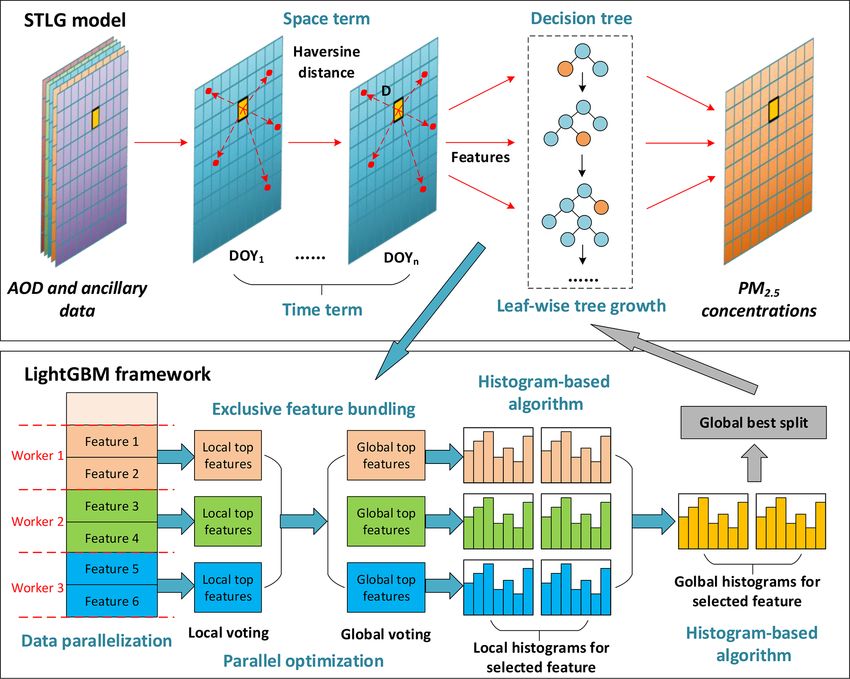
7866 J. Wei et al.: Hourly PM2.5 mapping across China using the space-time LightGBM model
Table 1. Summary of datasets and sources used in this study. CNEMC is the China National Environmental Monitoring Center.
Dataset Variable Content Unit Spatial resolution Temporal resolution Data source
PM2.5 PM2.5 PM2.5 µg m−3 In situ Hourly CNEMC
AOD AOD Himawari-8 AOD – 5 km × 5 km Hourly Himawari-8
Meteorology ET Total evaporation mm 0.1◦ × 0.1◦ Hourly ERA5
SP Surface pressure hPa 0.1◦ × 0.1◦
TEM 2 m temperature K 0.1◦ × 0.1◦
WU 10 m u-component of wind m s−1 0.1◦ × 0.1◦
WV 10 m v-component of wind m s−1 0.1◦ × 0.1◦
BLH Boundary-layer height m 0.25◦ × 0.25◦
RH Relative humidity % 0.25◦ × 0.25◦
Emissions NH3 Ammonia Mg grid−1 0.25◦ × 0.25◦ Monthly MEIC
NOx Nitrogen oxides Mg grid−1
SO2 Sulfur dioxide Mg grid−1
VOC Volatile organic compounds Mg grid−1
PM PM, coarse Mg grid−1
Land cover NDVI NDVI – 0.05◦ × 0.05◦ Monthly MOD13C2
Topography DEM Surface elevation m 90 m × 90 m – SRTM
Population POP Ambient population – 1 km × 1 km Yearly LandScan™
where ϕ and γ represent the latitude and longitude of a point 3 Results and discussion
on the sphere, respectively, and r denotes Earth’s mean ra-
dius (≈ 6371 km). Figure 1 illustrates the flowchart of the 3.1 Model fitting and validation
new STLG model.
In addition to Himawari-8 AODs, other auxiliary variables 3.1.1 Spatial-scale performance
were considered and employed to improve PM2.5 –AOD rela-
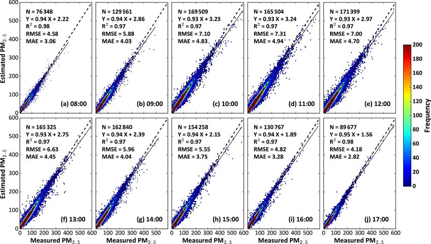
The STLG model can largely minimize overfitting, showing
tionships. However, to avoid redundant information, we first
a strong data-mining ability (Fig. 3) which can more accu-
calculated the normalized importance (%) of each feature to
rately establish the relationships between hourly PM2.5 ob-
the PM2.5 estimation during the model training (Fig. 2). It
servations and influential variables (i.e., coefficient of deter-
represents the total gains of splits that use the feature dur-
mination, R 2 = 0.97–0.98, RMSE = 4.18–7.31 µg m−3 ). Fig-
ing the decision-tree construction but not the physical contri-
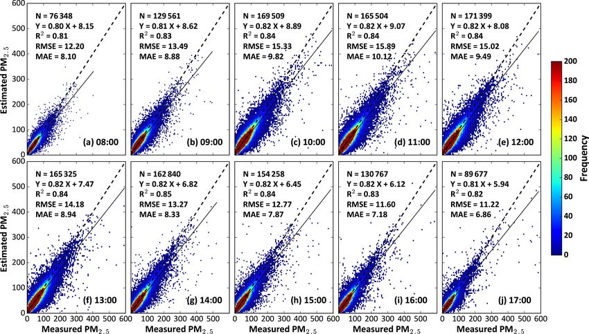
ure 4 illustrates the out-of-sample evaluation results of es-
bution. AOD is found to be the most important feature, ac-
timated hourly PM2.5 values over China from 08:00 to
counting for about 17 %. All meteorological factors have an
17:00 LT in 2018. The STLG model is highly accurate in esti-
important impact on the PM2.5 estimation, especially BLH,
mating hourly PM2.5 concentrations, with high sample-based
RH, and TEM (importance > 8 %), followed by two surface-
CV-R 2 values ranging from 0.81 to 0.85, strong slopes of
related variables (i.e., NDVI and DEM) and POP. The influ-
∼ 0.81–0.84, and small y-intercepts of ∼ 5.52–7.84 µg m−3 .
ence of aerosol precursors and emissions (i.e., NH3 , NOx ,
The uncertainties are overall small, with RMSEs (MAEs)
SO2 , PM, and VOC) on the PM2.5 estimation cannot be ig-
ranging from 11.24 (6.82) µg m−3 to 15.56 (9.79) µg m−3 .
nored (importance > 2 %). Therefore, all 16 selected vari-
However, the STLG performs slightly differently with small
ables are included to establish the final model in this study.
differences in main evaluation indicators throughout the day.
Here, two independent 10-fold cross-validation methods
The main reason being that the number of training samples
(10-CV) (Rodriguez et al., 2010) based on all the data sam-
is reduced during sunrise (Fig. 4a and b) and sunset (Fig. 4i
ples (i.e., out-of-sample) and PM2.5 monitoring stations (i.e.,
and j) in optical remote sensing, affecting the model train-
out-of-station) were selected to validate the model perfor-
ing. Air pollution also has clear diurnal variations at different
mance and the spatial prediction ability, respectively.
PM2.5 pollution levels due to the different intensities of hu-
man activities and natural conditions. In general, our model
is stable and robust, with an equal out-of-sample CV-R 2 of
0.85 and an equal regression slope of 0.81 at most hours dur-
ing the day in China (Fig. 4c–h).
Atmos. Chem. Phys., 21, 7863–7880, 2021 https://doi.org/10.5194/acp-21-7863-2021
J. Wei et al.: Hourly PM2.5 mapping across China using the space-time LightGBM model                                          7867

Figure 1. Schematics of the space-time LightGBM (STLG) model developed in this study (upper panel) and the framework of the original
LightGBM model (bottom panel).

                                                                    servations.. The station-based accuracy is also slightly de-
                                                                    creased with reference to the sample-based accuracy, fur-
                                                                    ther illustrating the robustness of our model. However, two
                                                                    cross-validation results (e.g., slopes = 0.78–0.84) indicate
                                                                    that hourly PM2.5 concentrations are overall underestimated
                                                                    (Figs. 4–5), a common issue in fine-particle remote sensing
                                                                    (Wei et al., 2020). This can be explained by the large aerosol
                                                                    retrieval uncertainty, as well as the small number of data sam-
                                                                    ples under highly polluted conditions (Wei et al., 2019c, d).
                                                                       The regional performance of the STLG model for hourly
                                                                    PM2.5 estimates (Fig. 6) was also evaluated. Hourly PM2.5
                                                                    estimates (number of data samples, N = 1 151 595) are
                                                                    highly consistent with ground measurements, with a high
                                                                    sample-based CV-R 2 of 0.87 and a strong regression
                                                                    slope of 0.86, showing small estimation uncertainties (i.e.,
                                                                    RMSE = 12.77 µg m−3 , MAE = 8.12 µg m−3 ) over eastern
Figure 2. Sorted normalized importance (%) of each feature in the   China. The STLG model performs well (e.g., CV-R 2 = 0.88,
PM2.5 estimation during the model construction.                     slope = 0.87) in two typical urban agglomerations of pub-
                                                                    lic concern in China, i.e., the Beijing–Tianjin–Hebei (BTH)
                                                                    (Fig. 6b) and Yangtze River Delta (YRD) (Fig. 6c) regions.
                                                                    By contrast, our model performs relatively poorly in the Pearl
   Furthermore, out-of-station CV-R 2 values range from             River Delta (PRD) region (Fig. 6d) possibly due to the sig-
0.76 to 0.81, and RMSE (MAE) values range from 12.49                nificant reduction in the number of data samples caused by
(7.85) µg m−3 to 17.61 (11.33) µg m−3 (Fig. 5), indicating          frequent, long-term cloud cover in southern China. Note that
that our model has a strong spatial prediction ability and can      there are some differences in the uncertainty of hourly PM2.5
predict PM2.5 values well in those areas without surface ob-

https://doi.org/10.5194/acp-21-7863-2021                                             Atmos. Chem. Phys., 21, 7863–7880, 2021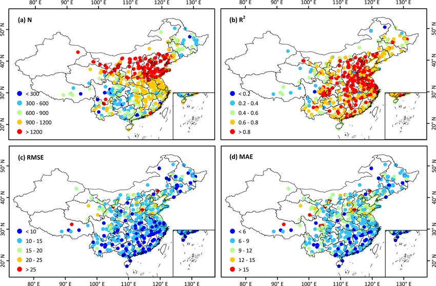
7868                               J. Wei et al.: Hourly PM2.5 mapping across China using the space-time LightGBM model

Figure 3. Density scatterplots of model-fitted PM2.5 estimates (µg m−3 ) at (a) 08:00 LT, (b) 09:00 LT, (c) 10:00 LT, (d) 11:00 LT, (e) 12:00 LT,
(f) 13:00 LT, (g) 14:00 LT, (h) 15:00 LT, (i) 16:00 LT, and (j) 17:00 LT in 2018 in China. Dashed lines denote 1 : 1 lines, and solid lines denote
best-fit lines from linear regression.

Figure 4. Density scatterplots of out-of-sample cross-validation results of PM2.5 estimates (µg m−3 ) at (a) 08:00 LT, (b) 09:00 LT,
(c) 10:00 LT, (d) 11:00 LT, (e) 12:00 LT, (f) 13:00 LT, (g) 14:00 LT, (h) 15:00 LT, (i) 16:00 LT, and (j) 17:00 LT in 2018 in China. Dashed
lines denote 1 : 1 lines, and solid lines denote best-fit lines from linear regression.

Atmos. Chem. Phys., 21, 7863–7880, 2021                                                        https://doi.org/10.5194/acp-21-7863-2021
J. Wei et al.: Hourly PM2.5 mapping across China using the space-time LightGBM model                                                     7869

Figure 5. Density scatterplots of out-of-station cross-validation results of PM2.5 estimates (µg m−3 ) at (a) 08:00 LT, (b) 09:00 LT,
(c) 10:00 LT, (d) 11:00 LT, (e) 12:00 LT, (f) 13:00 LT, (g) 14:00 LT, (h) 15:00 LT, (i) 16:00 LT, and (j) 17:00 LT in 2018 in China. Dashed and
solid lines denote 1 : 1 and best-fit lines from linear regression, respectively.

estimates mainly because of varying levels of air pollution.
The pollution level in the BTH region is about 3 times higher
than that in the PRD region.
   Figure 7 shows the accuracy of the STLG model at
each monitoring station across China. At the individual
site scale, the number of data samples gradually decreases
from northern China to southern China mainly due to in-
creasing cloud contamination with a site average of 997
data samples in China. Except for several scattered mon-
itoring stations in western China, the STLG model has
a high performance and adaptability and can estimate
well hourly PM2.5 concentrations at most monitoring sta-
tions (e.g., average CV-R 2 = 0.78, RMSE = 12.21 µg m−3 ,
and MAE = 8.17 µg m−3 ). In general, approximately 76 %,
79 %, and 82 % of monitoring stations show high accu-
racy, with out-of-sample CV-R 2 values > 0.7, RMSE val-
ues < 15 µg m−3 , and MAE values < 10 µg m−3 in hourly
PM2.5 estimates, especially for those located in central and
northern China.

3.1.2   Temporal-scale performance                                        Figure 6. Density scatterplots of out-of-sample cross-validation re-
                                                                          sults of hourly PM2.5 estimates (µg m−3 ) in 2018 for (a) eastern
We first quantified the time series of the bias in hourly PM2.5           China, (b) the Beijing–Tianjin–Hebei (BTH) region, (c) the Yangtze
estimates during the day in China (Fig. 8). There is a slight             River Delta (YRD), and (d) the Pearl River Delta (PRD) in China.
temporal dependence in that the PM2.5 bias increases gradu-
ally with increasing standard deviation, reaching a maximum
around 11:00 LT and subsequently decreasing. This seems to                trations. The PM2.5 estimates are less affected by the time-
be closely related to the diurnal variation in PM2.5 concen-              dependent bias in the Himawari-8 AOD product (Wei et al.,

https://doi.org/10.5194/acp-21-7863-2021                                                    Atmos. Chem. Phys., 21, 7863–7880, 2021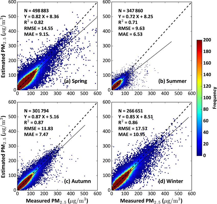
7870                               J. Wei et al.: Hourly PM2.5 mapping across China using the space-time LightGBM model

Figure 7. Individual-site-scale validation of hourly PM2.5 estimates (µg m−3 ) in 2018 in China in terms of (a) the sample size (N), (b) CV-R 2 ,
(c) RMSE, and (d) MAE.

2019c) because machine learning is not sensitive to the sys-
tematic bias of aerosol retrievals (Wei et al., 2021c). Nev-
ertheless, our model is generally robust and can accurately
estimate PM2.5 concentrations with small mean (median) bi-
ases of 0.05–0.08 (0.63–0.99) µg m−3 during different hours
throughout the day.
   We also compared Himawari-8-derived and ground-based
PM2.5 diurnal variations from all available monitoring sta-
tions in China and three typical urban clusters (Fig. 9).
Hourly PM2.5 concentrations observed by satellite are highly
consistent with ground-based measurements, with a small
difference within ± 0.10, 0.11, 0.13, and 0.11 µg m−3 in
China and in each region. Moreover, the same diurnal vari-                 Figure 8. Boxplots of the temporal dependence of the bias in hourly
ations in PM2.5 pollution are seen during the day; i.e., they              PM2.5 estimates (µg m−3 ) in 2018 in China. In each box, the red dot
reach their maximum values at 10:00 or 11:00 LT and are                    represents the mean bias, and the middle, lower, and upper horizon-
lower at sunrise and sunset. These results illustrate that the             tal blue lines represent the median bias, 25th percentile, and 75th
diurnal PM2.5 variations derived from Himawari-8 are rea-                  percentile, respectively.
sonable compared to ground-based measurements.
   We investigated the time series of the daily performance
of the STLG model in estimating hourly PM2.5 concentra-
tions in China. The number of data samples varies on a                     by different degrees of cloud contamination in the satellite
daily basis, with an average of 3975 d−1 and with more                     aerosol products for different days. The STLG model cap-
than 83 % of all days having more than 2000 (Fig. 10). The                 tures well the hourly PM2.5 values on most days, with an
large gap in the number of data samples is mainly caused                   average out-of-sample R 2 of 0.73 and average RMSE and
                                                                           MAE values of 13.06 and 8.53 µg m−3 , respectively. In gen-

Atmos. Chem. Phys., 21, 7863–7880, 2021                                                       https://doi.org/10.5194/acp-21-7863-2021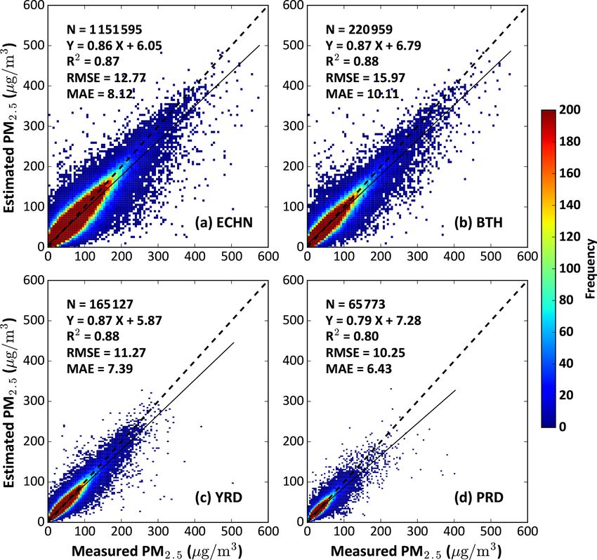
J. Wei et al.: Hourly PM2.5 mapping across China using the space-time LightGBM model                                               7871

Figure 9. Time series of Himawari-8-derived (blue bars) and ground-based (orange bars) PM2.5 diurnal variations (µg m−3 ) in (a) China,
(b) the Beijing–Tianjin–Hebei (BTH) region, (c) the Yangtze River Delta (YRD), and (d) the Pearl River Delta (PRD).

Figure 10. Time series of out-of-sample cross validation of hourly PM2.5 estimates (µg m−3 ) in terms of (a) the sample size (N, red) and
CV-R 2 (blue) and (b) RMSE (red) and MAE (blue) in 2018 in China.

eral, hourly PM2.5 estimates are more reliable on approxi-             In general, the overall uncertainty of PM2.5 estimates in-
mately 79 % (CV-R 2 > 0.7), 70 % (RMSE < 15 µg m−3 ), and              creases at the beginning and at the end of the year likely
74 % (MAE < 10 µg m−3 ) of the days in the year. The model             due to the harsher environmental conditions (e.g., low hu-
performance also varies greatly at the seasonal level, with            midity and less precipitation) and more intense human ac-
average CV-R 2 values of 0.82, 0.71, 0.87, and 0.86 and aver-          tivities (e.g., coal heating and straw burning) in winter and
age RMSE values of 14.55, 9.63, 11.83, and 17.57 µg m−3 in             spring.
spring, summer, autumn, and winter, respectively (Fig. 11).

https://doi.org/10.5194/acp-21-7863-2021                                                 Atmos. Chem. Phys., 21, 7863–7880, 2021
7872 J. Wei et al.: Hourly PM2.5 mapping across China using the space-time LightGBM model
Figure 12. Density scatterplots of out-of-sample cross-validation
results of (a) daily, (b) monthly, (c) seasonal, and (d) annual mean
Figure 11. Density scatterplots of out-of-sample cross-validation
PM2.5 estimates (µg m−3 ) in 2018 across China.
results of hourly PM2.5 estimates (µg m−3 ) for (a) spring, (b) sum-
mer, (c) autumn, and (d) winter of 2018 in China. Dashed and solid
lines denote 1 : 1 and best-fit lines from linear regression, respec-
tively.
can last several hours. As the day progresses, human activi-
ties subside, and atmospheric fine particles settle on surfaces.
PM2.5 concentrations thus decrease towards sunset in most
We have evaluated temporally synthesized PM2.5 data
areas in China (∼ 23.21 ± 9.73 µg m−3 ). In general, air pol-
from the hourly data samples at each monitoring station for
lution in the morning (i.e., 08:00–12:00 LT) is much more
the year 2018 (Fig. 12). Daily mean PM2.5 estimates are
severe than in the afternoon (i.e., 13:00–17:00 LT) in China,
highly correlated to those calculated from surface observa-
with morning PM2.5 concentrations about 1.3 times higher
tions (R 2 = 0.91), and the average RMSE (MAE) value is
than afternoon levels. This is related to the influence of vary-
10.11 (6.39) µg m−3 . This suggests that the STLG model
ing BLHs (Z. Li et al., 2017; Su et al., 2018).
can capture daily PM2.5 variations more accurately. Note that
Table 2 summarizes the diurnal PM2.5 variations in eastern
daily synthetic PM2.5 data derived from geostationary satel-
China and three typical urban agglomerations. PM2.5 pollu-
lites have a higher temporal frequency than data derived from
tion levels in eastern China are generally higher than the na-
sun-synchronous satellites. In general, PM2.5 synthetic val-
tional level at each hour of the day due to the dense human
ues also have high accuracies and low estimation uncertain-
population and intensive human activities. In the BTH re-
ties (e.g., R 2 = 0.98, RMSE = 1.6–3.3 µg m−3 , MAE = 1.1–
gion, PM2.5 pollution varies greatly, with hourly PM2.5 con-
2.3 µg m−3 ) from monthly to annual scales, allowing for a
centrations ranging from 28.88 ± 10.16 µg m−3 (10:00 LT)
better description of spatiotemporal distributions and varia-
to 49.31 ± 15.03 µg m−3 (16:00 LT) and with differences ex-
tions in PM2.5 pollution across China.
ceeding 20 µg m−3 . PM2.5 pollution remained at a high level
3.2 Spatiotemporal characteristics (> 42 µg m−3 ) before 12:00 LT and dropped to a lower level
(< 29 µg m−3 ) after 16:00 LT. This is closely related to peo-
3.2.1 Diurnal variations ple’s daily activities and the production and life cycle of
PM2.5 during the day, as well as the change in boundary mix-
Figure 13 shows Himawari-8-derived hourly mean near- ing as a function of the day (Lennartson et al., 2018; Wang
surface PM2.5 concentrations from 08:00 to 17:00 LT in 2018 and Christopher, 2003). Similar patterns and PM2.5 pollution
across mainland China. They do not cover western Xinjiang levels are seen in the YRD region. In general, the PRD re-
and Tibet due to the limitation of satellite scanning. PM2.5 gion is less polluted in the morning but more severely pol-
pollution varies diurnally across China, being at an overall luted in the afternoon than the BTH region. Compared with
low level at sunrise (∼ 29.94 ± 10.91 µg m−3 ). With the in- the BTH and PRD regions, PM2.5 pollution in the PRD re-
crease in human activities, air pollution becomes more se- gion is much lower and shows a smaller diurnal difference,
vere over time, reaching a peak at around 10:00–11:00 LT with hourly PM2.5 values ranging from 29.49 ± 5.97 µg m−3
in China (∼ 36 ± 13 µg m−3 ). These high levels of pollution (11:00 LT) to 36.36 ± 5.76 µg m−3 (08:00 LT). Better natural
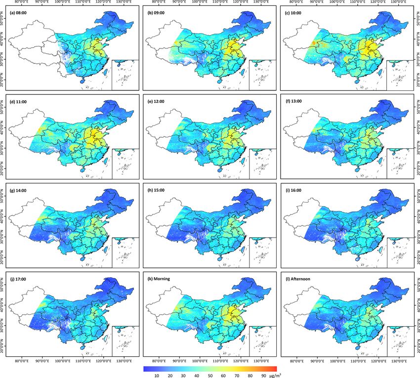
Atmos. Chem. Phys., 21, 7863–7880, 2021 https://doi.org/10.5194/acp-21-7863-2021J. Wei et al.: Hourly PM2.5 mapping across China using the space-time LightGBM model 7873 Figure 13. Himawari-8-derived hourly mean PM2.5 maps (5 km) for different times of the day: (a) 08:00 LT, (b) 09:00 LT, (c) 10:00 LT, (d) 11:00 LT, (e) 12:00 LT, (f) 13:00 LT, (g) 14:00 LT, (h) 15:00 LT, (i) 16:00 LT, (j) 17:00 LT, (k) morning (08:00–12:00 LT), and (l) afternoon (13:00–17:00 LT) in 2018 across China. conditions and fewer pollutant emissions mainly explain this rate information about the distribution of and variations in (Su et al., 2018). PM2.5 pollution. In general, our satellite-derived diurnal variations in PM2.5 pollution agree well with ground-based observations at both 3.2.2 Seasonal and annual variations national and regional levels but with generally lower PM2.5 concentrations (Fig. 9). The reason is that the PM2.5 mon- Seasonal PM2.5 maps are synthesized from daily PM2.5 itoring stations are unevenly distributed and vary greatly in maps from 2018 across China according to our previ- the number of stations at the regional scale. Also, most sites ous approach (Wei et al., 2019a). Our results illustrate are distributed in urban areas, leading to inevitable overes- that PM2.5 pollution varies greatly on a seasonal scale timations due to urban–rural differences. However, satellite (Fig. 14). Pollution levels are generally low and show remote sensing can cope with this deficiency by generat- similar spatial patterns in summer (∼ 22.86 ± 7.05 µg m−3 ) ing spatially continuous PM2.5 maps, providing more accu- and autumn (∼ 23.76 ± 10.97 µg m−3 ) across China https://doi.org/10.5194/acp-21-7863-2021 Atmos. Chem. Phys., 21, 7863–7880, 2021
7874                             J. Wei et al.: Hourly PM2.5 mapping across China using the space-time LightGBM model

Table 2. Hourly mean PM2.5 concentrations (µg m−3 ) in 2018 in China, eastern China (ECHN), the Beijing–Tianjin–Hebei (BTH) region,
the Yangtze River Delta (YRD), and the Pearl River Delta (PRD).

                     Time                China           ECHN              BTH             YRD            PRD
                     08:00       29.94 ± 10.91    31.97 ± 11.55    42.46 ± 12.97   38.60 ± 10.57   29.34 ± 5.01
                     09:00       33.37 ± 12.59    36.29 ± 13.52    47.32 ± 15.04   43.55 ± 11.27   34.81 ± 5.46
                     10:00       35.67 ± 13.53    38.56 ± 14.05    49.31 ± 15.03   44.72 ± 11.17   35.48 ± 5.47
                     11:00       35.63 ± 13.05    38.72 ± 13.53    49.10 ± 13.77   44.27 ± 10.55   36.36 ± 5.76
                     12:00       31.23 ± 11.74    35.10 ± 12.47    42.38 ± 12.86    41.37 ± 9.77   34.56 ± 5.72
                     13:00       28.45 ± 11.40    32.23 ± 11.73    37.70 ± 11.55    39.36 ± 9.22   33.33 ± 5.48
                     14:00       26.36 ± 11.18    30.14 ± 11.09    34.32 ± 11.81    37.31 ± 8.59   32.05 ± 5.50
                     15:00       24.25 ± 10.06    28.67 ± 10.21    31.95 ± 11.26    36.77 ± 8.13   30.34 ± 5.43
                     16:00        23.63 ± 9.26     27.38 ± 9.15    29.82 ± 10.13    32.84 ± 6.30   29.49 ± 5.97
                     17:00        23.21 ± 9.73     26.63 ± 8.93    28.88 ± 10.16    27.59 ± 4.39   31.56 ± 6.17
                     Morning     33.29 ± 11.59    36.15 ± 12.41    46.12 ± 13.29   42.50 ± 10.22   34.52 ± 4.63
                     Afternoon    25.11 ± 9.78     29.01 ± 9.70    32.53 ± 10.53    34.76 ± 6.66   31.42 ± 4.85

(Table 3). By contrast, it is much more severe                       estimation uncertainties because of their nonlinear charac-
in     spring    (∼ 32.84 ± 11.49 µg m−3 )       and     winter      teristics and stronger data regression abilities. The two-stage
(∼ 39.04 ± 16.32 µg m−3 ) across China, especially in                model outperforms the GAM and maximum likelihood esti-
the BTH and YRD regions in winter. The main reasons are              mation (MLE) models with higher CV-R 2 values and smaller
the frequent sandstorms and the long-distance transmission           estimation uncertainties by combining the advantages of the
of sand and dust in spring and the burning of coal and               GWR and LME models. Our model performs better than
fossil fuels for heating in winter leading to more pollutant         all of the traditional statistical regression models considered
emissions in northern China.                                         mainly due to its stronger data-mining ability.
   PM2.5 pollution also shows significant spatial hetero-               The first six rows of Table 5 show the accuracies and ef-
geneities across China (Fig. 15), with an annual mean PM2.5          ficiencies of six tree-based machine-learning models when
concentration of 28.99 ± 10.31 µg m−3 in 2018 (Table 3).             estimating PM2.5 in China using the same input dataset.
High pollution levels are always observed in the Hebei,              The decision tree (DT; Quinlan, 1986) is a traditional, fre-
Shandong, Jiangsu, Anhui, Henan, Hubei, and Sichuan                  quently used, supervised learning classification method. Al-
provinces. Interactions between intensive human activities,          though the training speed is the fastest and the memory
adverse stagnant weather (e.g., low BLHs and low winds),             consumption is the least, it has the worst performance be-
and special terrain (e.g., basin) can increase anthropogenic         cause of the simple single classifier. The model perfor-
aerosols (Chen et al., 2008; Wang et al., 2018). By contrast,        mances of ensemble-learning approaches, i.e., GBDT (Fried-
PM2.5 pollution is relatively light in the northeast (e.g., Hei-     man, 2001), RF (Breiman, 2001), extremely randomized
longjiang and Jilin provinces), the southwest (e.g., Tibet and       trees (ERTs; Geurts et al., 2006), and XGBoost (Chen and
Yunnan provinces), and the eastern coastal areas of China            Guestrin, 2016), can be significantly improved by combin-
(e.g., Zhejiang and Fujian provinces). These provinces are           ing several weak classifiers into a strong classifier. Among
sparsely populated or experience meteorological conditions           them, the ERT model yields a higher estimation accuracy
favorable for dispersing pollution (Su et al., 2018).                and a stronger spatial prediction ability than other ensemble-
                                                                     learning models. The LightGBM model (Ke et al., 2017) per-
3.3     Discussion                                                   forms the best with the highest accuracy and smallest un-
                                                                     certainty among all tree-based machine-learning approaches
3.3.1    Comparison with traditional models                          considered.
                                                                        The model efficiency differs among these models due to
We first compared results from the STLG model with results           the large differences in the algorithm design frameworks.
from five widely used statistical regression models employed         These tree-based machine-learning models can be divided
for estimating PM2.5 in China using the same input dataset           into two categories. The DT, RF, and ERT models fall into the
(Table 4). The multivariate linear regression (MLR) model            “bagging” category, which synthesizes multiple independent
performs the worst due to the complex nonlinear PM2.5 –              and unrelated weak classifiers into a strong classifier. It al-
AOD relationship. The GWR model performs better because              lows for work in parallel, which can save much time but may
it takes into account the spatial characteristics of PM2.5 pol-      need more computer memory. The GBDT, XGBoost, and
lution. The generalized additive model (GAM) and the LME             LightGBM models fall into the “boosting” category, which
model show overall improved performances with decreasing             synthesizes multiple interdependent and related weak clas-

Atmos. Chem. Phys., 21, 7863–7880, 2021                                               https://doi.org/10.5194/acp-21-7863-2021
J. Wei et al.: Hourly PM2.5 mapping across China using the space-time LightGBM model 7875
Figure 14. Himawari-8-derived seasonal mean PM2.5 maps (5 km) for (a) spring, (b) summer, (c) autumn, and (d) winter of 2018 across
China.
Table 3. Annual and seasonal mean PM2.5 concentrations (µg m−3 ) in 2018 in China, eastern China (ECHN), the Beijing–Tianjin–Hebei
(BTH) region, the Yangtze River Delta (YRD), and the Pearl River Delta (PRD).
Time China ECHN BTH YRD PRD
Spring 32.84 ± 11.49 34.93 ± 10.95 45.75 ± 12.96 40.35 ± 9.55 33.97 ± 4.50
Summer 22.86 ± 7.05 24.16 ± 6.29 29.99 ± 7.46 26.16 ± 4.58 23.56 ± 3.18
Autumn 23.76 ± 10.97 28.64 ± 11.60 35.98 ± 11.20 35.97 ± 7.80 29.54 ± 4.43
Winter 39.04 ± 16.32 48.34 ± 17.47 48.36 ± 18.92 57.41 ± 16.88 43.92 ± 8.56
Annual 28.99 ± 10.31 32.56 ± 10.78 39.32 ± 11.74 38.64 ± 8.27 32.98 ± 4.53
sifiers into a strong classifier. They can only work in serial, ing hourly PM2.5 concentrations with reference to their orig-
which may take much time but not too much memory. In gen- inal models. This further illustrates the importance of includ-
eral, the STGB model is the most time-consuming, while the ing spatiotemporal information when constructing PM2.5 –
STET model is the most memory-consuming. By contrast, AOD relationships. More importantly, the training speed
the LightGBM model runs very fast and consumes very lit- of these models did not decrease much, and the memory
tle computer memory, benefiting from a series of algorithm consumption did not increase much either. In general, the
optimizations (Ke et al., 2017). STLG model shows the best performance with a high effi-
After considering spatiotemporal variations, all the newly ciency (i.e., training speed = 46 s, memory usage = 0.60 GB)
defined space-time DT, GBDT, XGBoost, RF, ERT, and among all the space-time tree-based machine-learning mod-
LightGBM models (i.e., STDT, STGB, STXB, STRF, STET, els. Therefore, our new STLG model is highly valuable for
and STLG) show significant improvements in both overall accurate and fast air pollution monitoring, in particular for
estimation accuracy and spatial prediction ability in estimat- our future study extended to the global scale.
https://doi.org/10.5194/acp-21-7863-2021 Atmos. Chem. Phys., 21, 7863–7880, 20217876 J. Wei et al.: Hourly PM2.5 mapping across China using the space-time LightGBM model
Figure 15. Himawari-8-derived annual mean PM2.5 map (5 km) for the year 2018 across China. The lower-left-inserted density scatterplot
represents out-of-sample cross-validation results for all hourly PM2.5 estimates in China.
Table 4. Comparison of the model performances of widely used e.g., the I-LME, IGTWR, RF, AdaBoost, XGBoost, and their
models and the STLG model in estimating PM2.5 from Himawari-8 stacked models in China (Chen et al., 2019; Liu et al., 2019;
data at 14:00 LT in 2018 in China (N = 162 840). Xue et al., 2020; T. Zhang et al., 2019). This is due to the
stronger data-mining ability, considering key spatial and tem-
Model Out-of-sample validation Out-of-station validation poral information about air pollution (ignored in previous
CV-R 2 RMSE MAE CV-R 2 RMSE MAE studies), which introduces more comprehensive factors that
MLR 0.19 24.17 22.89 0.19 24.19 22.91
affect PM2.5 pollution (e.g., emission inventories).
GWR 0.39 21.96 20.74 0.37 22.42 21.02
GAM 0.39 19.09 18.64 0.36 19.77 18.89
LME 0.50 18.91 17.34 0.48 19.06 17.95 4 Summary and conclusion
Two-stage 0.58 17.60 15.71 0.54 17.99 16.01
STLG 0.85 13.09 8.11 0.81 14.63 9.29 PM2.5 has a great impact on the atmospheric environment
and is also used as a key indicator in environmental health
studies. It varies diurnally, affected by both natural and hu-
3.3.2 Comparison with related studies man factors. Previous studies have been based on data from
sun-synchronous satellites which can monitor air pollution
We compared Himawari-8-based hourly PM2.5 estimates at at coarse temporal scales (i.e., daily), while high-temporal-
regional and national scales in China with previous related resolution and accurate information on PM2.5 is needed. In
studies (Table 6). Local hourly PM2.5 concentrations re- this study, the Himawari-8/AHI hourly AOD product is em-
trieved from our national-scale model are more accurate than ployed to address this issue. Moreover, considering the large
those derived from the models developed separately in local volume of input data and the large errors in PM2.5 estimation
areas, e.g., the LME model (Wang et al., 2017), the GWR, using traditional methods, an efficient and accurate space-
SVR, RF, and DNN models in the BTH region (Sun et al., time Light Gradient Boosting Machine (i.e., STLG) model
2019) and the two-stage RF and DNN models in the YRD has been developed. It utilizes meteorological, human, land
region (Fan et al., 2020; Tang et al., 2019). Our model also use, and topographical parameters and is implemented at
outperforms most of the statistical regression models and 5 km resolution and hourly timescale to generate PM2.5 in-
machine-learning models focused on the entirety of China, formation over China. The hourly PM2.5 estimates are evalu-
Atmos. Chem. Phys., 21, 7863–7880, 2021 https://doi.org/10.5194/acp-21-7863-2021J. Wei et al.: Hourly PM2.5 mapping across China using the space-time LightGBM model 7877
Table 5. Comparison of the model performances of different tree-based machine-learning models and the STLG model using the same input
data. Data are from 14:00 LT in 2018 in China (N = 162 840). TSpeed and TMemory refer to the speed and memory consumption during the
model training.
Model Out-of-sample validation Out-of-station validation TSpeed TMemory
R2 RMSE MAE R2 RMSE MAE (s) (GB)
DT 0.52 25.53 14.80 0.48 27.03 15.57 6 0.58
GBDT 0.65 20.03 13.17 0.61 21.20 14.10 94 0.59
XGBoost 0.73 17.94 10.78 0.68 19.59 11.93 456 0.69
RF 0.72 17.86 11.33 0.69 18.80 11.95 165 2.59
ERT 0.74 17.12 10.87 0.72 18.01 11.49 54 3.69
LightGBM 0.78 15.79 9.84 0.73 17.59 11.21 34 0.60
STDT 0.65 21.09 12.33 0.63 22.00 12.85 8 0.60
STGB 0.75 16.82 10.93 0.73 17.61 11.54 503 0.61
STXB 0.82 14.73 8.76 0.78 15.92 9.62 456 0.68
STRF 0.81 14.62 9.17 0.79 15.44 9.69 219 2.75
STET 0.82 14.42 8.95 0.80 15.30 9.55 77 4.25
STLG 0.85 13.09 8.11 0.81 14.63 9.29 46 0.60
Table 6. Comparison of model performances from previous studies in estimating hourly PM2.5 concentrations in China.
Model Model validation Region Reference
R2 RMSE MAE
LME 0.86 24.5 14.2 BTH Wang et al. (2017)
LME 0.63 29.0 18.1 BTH Sun et al. (2019)
GWR 0.76 23.3 16.7 Sun et al. (2019)
SVR 0.77 21.5 12.3 Sun et al. (2019)
RF 0.82 20.3 12.1 Sun et al. (2019)
DNN 0.84 19.9 11.9 Sun et al. (2019)
two-stage RF 0.86 12.4 – YRD Tang et al. (2019)
DNN 0.86 14.3 – YRD Fan et al. (2020)
RF 0.82 19.6 12.2 China Chen et al. (2019)
AdaBoost 0.84 18.3 10.7 Chen et al. (2019)
XGBoost 0.84 18.1 11.4 Chen et al. (2019)
Stacked model 0.85 17.3 10.5 Chen et al. (2019)
RF 0.86 17.3 10.3 China Liu et al. (2019)
I-LME 0.84 – – BTH T. Zhang et al. (2019)
0.80 – – YRD
0.74 – – PRD
0.82 – – China
IGTWR 0.78 21.1 – China Xue et al. (2020)
ated against surface observations, and PM2.5 spatiotemporal PM2.5 also varies greatly on a seasonal basis, in which win-
variations are also investigated. ter and summer experience the highest and lowest air pollu-
The STLG model predicts hourly PM2.5 values accu- tion levels, respectively. Comparison results suggest that the
rately, with high out-of-sample (out-of-station) CV-R 2 val- proposed model is more accurate than traditional statistical
ues of ∼ 0.81–0.85 (∼ 0.76–0.81) and low RMSE values regression models, other tree-based machine-learning mod-
of ∼ 11.24–15.56 (∼ 12.49–17.61) µg m−3 throughout the els, and various models developed in previous studies. Over-
day. The model can also produce daily (e.g., R 2 = 0.91, all, the STLG model is more efficient, having faster training
RMSE = 10.11 µg m−3 ), monthly, seasonal, and annual mean speed and less memory consumption. These results illustrate
PM2.5 values (e.g., R 2 = 0.98, RMSE = 1.6–3.3 µg m−3 ). that this algorithm can be useful for real-time monitoring of
PM2.5 varies diurnally in most areas of mainland China, PM2.5 pollution in China.
where PM2.5 concentrations reach a maximum at 10:00 LT
and are generally low at sunrise and sunset on a given day.
https://doi.org/10.5194/acp-21-7863-2021 Atmos. Chem. Phys., 21, 7863–7880, 20217878 J. Wei et al.: Hourly PM2.5 mapping across China using the space-time LightGBM model
Data availability. PM2.5 measurements are available at http:// Bessho, K., Date, K., Hayashi, M., Ikeda, A., and Yoshida, R.: An
www.cnemc.cn (CNEMC, 2020), the Himawari-8 AOD product introduction to Himawari-8/9 – Japan’s new-generation geosta-
is available at https://www.eorc.jaxa.jp/ptree/ (JAXA Himawari tionary meteorological satellites, J. Meteorol. Soc. Jpn., 2016,
Monitor, 2020), ERA5 reanalysis products are available at https: 94, 151–183, 2016.
//cds.climate.copernicus.eu/ (CDS, 2020), the MODIS product is Breiman, L.: Random forests, Mach. Learn., 45, 5–32, 2001.
available at https://search.earthdata.nasa.gov/ (NASA, 2020), and CDS: ERA5, available at: https://cds.climate.copernicus.eu/, last
the LandScan™ product is available at https://landscan.ornl.gov/ access: 1 December 2020.
(ORNL, 2020). The ChinaHighPM2.5 dataset is available at https: Chan, C. and Yao, X.: Air pollution in megacities in China, Atmos.
//weijing-rs.github.io/product.html (Wei, 2020). Environ., 42, 1–42, 2008.
Chen, J., Yin, J., Zang, L., Zhang, T., and Zhao, M.: Stacking ma-
chine learning model for estimating hourly PM2.5 in China based
Author contributions. JiW designed the research and wrote the ini- on Himawari-8 aerosol optical depth data, Sci. Total Environ.,
tial draft of this manuscript. ZL, RTP, JuW, and LS reviewed and 697, 134021, https://doi.org/10.1016/j.scitotenv.2019.134021,
edited the paper. RL and WX helped to process the data. MC copy- 2019.
edited the article. All authors made substantial contributions to this Chen, T. and Guestrin, C.: XGBoost: a scalable tree boosting sys-
work. tem, in: Proceedings of the 22nd ACM SIGKDD International
Conference on Knowledge Discovery and Data Mining, 13–
17 August 2016, San Francisco, CA, USA, 785–794, 2016.
Competing interests. The authors declare that they have no conflict Chen, Z., Cheng, S., Li, J., Guo, X., Wang, W., and Chen, D.: Re-
of interest. lationship between atmospheric pollution processes and synoptic
pressure patterns in northern China, Atmos. Environ., 42, 6078–
6087, 2008.
CNEMC: http://www.cnemc.cn, last access: 1 December 2020.
Special issue statement. This article is part of the special issue
Delfino, R. J., Sioutas, C., and Malik, S.: Potential role of ultrafine
“Satellite and ground-based remote sensing of aerosol optical, phys-
particles in associations between airborne particle mass and car-
ical, and chemical properties over China”. It is not associated with
diovascular health, Environ. Health Persp., 113, 934–946, 2005.
a conference.
Dobson, J., Bright, E., Coleman, P., Durfee, R., and Worley, B.:
A global population database for estimating populations at risk,
Photogramm. Eng. Rem. S., 66, 849–857, 2000.
Acknowledgements. We would like to thank Qiang Zhang at Ts- Fan, W., Qin, K., Cui, Y., Li, D., and Bilal, M.: Estimation of
inghua University for providing MEIC pollution emission data for hourly ground-level PM2.5 concentration based on Himawari-
China. Jun Wang’s participation is made possible via the in-kind 8 apparent reflectance, IEEE T. Geosci. Remote, 59, 76–85,
support from the University of Iowa. https://doi.org/10.1109/TGRS.2020.2990791, 2020.
Friedman, J.: Greedy function approximation: a gradient boosting
machine, Ann. Stat., 29, 1189–1232, 2001.
Financial support. This research has been supported by the Na- Geurts, P., Ernst, D., and Wehenkel, L.: Extremely randomized
tional Natural Science Foundation of China (grant no. 42030606) trees, Mach. Learn., 63, 3–42, 2006.
and the National Key Research and Development Program of China Giles, D. M., Sinyuk, A., Sorokin, M. G., Schafer, J. S., Smirnov,
(grant no. 2017YFC1501702). A., Slutsker, I., Eck, T. F., Holben, B. N., Lewis, J. R., Campbell,
J. R., Welton, E. J., Korkin, S. V., and Lyapustin, A. I.: Advance-
ments in the Aerosol Robotic Network (AERONET) Version 3
Review statement. This paper was edited by Toshihiko Takemura database – automated near-real-time quality control algorithm
and reviewed by two anonymous referees. with improved cloud screening for Sun photometer aerosol op-
tical depth (AOD) measurements, Atmos. Meas. Tech., 12, 169–
209, https://doi.org/10.5194/amt-12-169-2019, 2019.
Gui, K., Che, H., Zeng, Z., Wang, Y., Zhai, S., Wang, Z., Luo, M.,
References Zhang, L., Liao, T., Zhao, H., Li, L., Zheng, Y., and Zhang, X.:
Construction of a virtual PM2.5 observation network in China
An, Z., Huang, R. J., Zhang, R., Tie, X., Li, G., Cao, J., Zhou, based on high-density surface meteorological observations us-
W., Shi, Z., Han, Y., Gu, Z., and Ji, Y.: Severe haze in northern ing the Extreme Gradient Boosting model, Environ. Int., 141,
China: a synergy of anthropogenic emissions and atmospheric 105801, https://doi.org/10.1016/j.envint.2020.105801, 2020.
processes, P. Natl. Acad. Sci. USA, 116, 8657–8666, 2019. Huang, R., Zhang, Y., Bozzetti, C., Ho, K., Cao, J., Han, Y., Dael-
Baez-Villanueva, O., Zambrano-Bigiarini, M., Beck, H., Mcna- lenbach, K., Slowik, J., Platt, S., Canonaco, F., Zotter, P., Wolf,
mara, I., and Thinh, N.: RF-MEP: a novel random forest R., Pieber, S., Bruns, E., Crippa, M., Ciarelli, G., Piazzalunga,
method for merging gridded precipitation products and ground- A., Schwikowski, M., Abbaszade, G., Schnelle-Kreis, J., Zim-
based measurements, Remote Sens. Environ., 239, 111606, mermann, R., An, Z., Szidat, S., Baltensperger, U., Haddad, I.,
https://doi.org/10.1016/j.rse.2019.111606, 2020. and Prevot, A.: High secondary aerosol contribution to particu-
Behrens, T., Schmidt, K., Viscarra, R., Gries, P., Scholten, T., and late pollution during haze events in China, Nature, 514, 218–222,
Macmillan, R.: Spatial modelling with Euclidean distance fields 2014.
and machine learning, Eur. J. Soil Sci., 69, 757–770, 2018.
Atmos. Chem. Phys., 21, 7863–7880, 2021 https://doi.org/10.5194/acp-21-7863-2021J. Wei et al.: Hourly PM2.5 mapping across China using the space-time LightGBM model 7879
Jacob, D. and Winner, D.: Effect of climate change on air quality, Liu, Y., Sarnat, J., Kilaru, V., Jacob, D., and Koutrakis, P.: Estimat-
Atmos. Environ., 43, 51–63, 2009. ing ground-level PM2.5 in the eastern United States using satel-
JAXA Himawari Monitor: https://www.eorc.jaxa.jp/ptree/, last ac- lite remote sensing, Environ. Sci. Technol., 39, 3269–78, 2005.
cess: 1 December 2020. Liu, Y., Franklin, M., Kahn, R., and Koutrakis, P.: Using aerosol
Kampa, M. and Castanas, E.: Human health effects of air pollution, optical thickness to predict ground-level PM2.5 concentrations
Environ. Pollut., 151, 362–367, 2008. in the St. Louis area: a comparison between MISR and MODIS.
Ke, G., Meng, Q., Finley, T., Wang, T., Chen, W., Ma, W., Ye, Remote Sens. Environ., 107, 33–44, 2007.
Q., and Liu, T.: LightGBM: a highly efficient gradient boost- Ma, Z., Hu, X., Huang, L., Bi, J., and Liu, Y.: Estimating ground-
ing decision tree, in: Advances in Neural Information Process- level PM2.5 in China using satellite remote sensing, Environ. Sci.
ing Systems, ACM, Long Beach, CA, USA, 3149–3157, avail- Technol., 48, 7436–7444, 2014.
able at: https://dl.acm.org/doi/10.5555/3294996.3295074 (last NASA: EARTHDATA, available at: https://search.earthdata.nasa.
access: 1 January 2020), 2017. gov/, last access: 1 December 2020.
Kim, K., Kabir, E., and Kabir, S.: A review on the human health ORNL: LandScan, available at: https://landscan.ornl.gov/, last ac-
impact of airborne particulate matter, Environ. Int., 74, 136–143, cess: 1 December 2020.
2015. Quinlan, J.: Induction on decision tree, Mach. Learn., 1, 81–106,
Lelieveld, J., Evans, J., Fnais, M., Giannadaki, D., and Pozzer, A.: 1986.
The contribution of outdoor air pollution sources to premature Ramanathan, V. and Feng, Y.: Air pollution, greenhouse gases and
mortality on a global scale, Nature, 525, 367–371, 2015. climate change: global and regional perspectives, Atmos. Envi-
Lennartson, E. M., Wang, J., Gu, J., Castro Garcia, L., Ge, C., ron., 43, 37–50, 2009.
Gao, M., Choi, M., Saide, P. E., Carmichael, G. R., Kim, J., and Rodriguez, J. D., Perez, A., and Lozano, J. A.: Sensitivity analysis
Janz, S. J.: Diurnal variation of aerosol optical depth and PM2.5 of k-fold cross-validation in prediction error estimation, IEEE T.
in South Korea: a synthesis from AERONET, satellite (GOCI), Pattern Anal., 32, 569–575, 2010.
KORUS-AQ observation, and the WRF-Chem model, Atmos. Shi, H.: Best-first decision tree learning, PhD thesis, The University
Chem. Phys., 18, 15125–15144, https://doi.org/10.5194/acp-18- of Waikato, Hamilton, New Zealand, 2007.
15125-2018, 2018. Su, T., Li, Z., and Kahn, R.: Relationships between the plan-
Letu, H., Yang, K., Nakajima, T., Ishimoto, H., Nagao, T., Riedi, J., etary boundary layer height and surface pollutants derived
Baran, A., Ma, R., Wang, T., Shang, H., Khatri, P., Chen, L., Shi, from lidar observations over China: regional pattern and in-
C., and Shi, J.: High-resolution retrieval of cloud microphysi- fluencing factors, Atmos. Chem. Phys., 18, 15921–15935,
cal properties and surface solar radiation using Himawari-8/AHI https://doi.org/10.5194/acp-18-15921-2018, 2018.
next-generation geostationary satellite, Remote Sens. Environ., Sun, Y., Zhuang, G., Wang, Y., Han, L., Guo, J., Dan, M., Zhang,
239, 111583, https://doi.org/10.1016/j.rse.2019.111583, 2020. W., Wang, Z., and Hao, Z.: The air-borne particulate pollution in
Li, M., Liu, H., Geng, G., Hong, C., Liu, F., Song, Y., Tong, D., Beijing – concentration, composition, distribution and sources,
Zheng, B., Cui, H., Man, H., Zhang, Q., and He, K.: Anthro- Atmos. Environ., 38, 5991–6004, 2004.
pogenic emission inventories in China: a review, Natl. Sci. Rev., Sun, Y., Zeng, Q., Geng, B., Lin, X., Sude, B., and Chen, L.: Deep
4, 834–866, https://doi.org/10.1093/nsr/nwx150, 2017. learning architecture for estimating hourly ground-level PM2.5
Li, Z., Guo, J., Ding, A., Liao, H., Liu, J., Sun, Y., Wang, T., Xue, using satellite remote sensing, IEEE Geosci. Remote S., 16,
H., Zhang, H., and Zhu, B.: Aerosols and boundary-layer inter- 1343–1347, 2019.
actions and impact on air quality, Natl. Sci. Rev., 4, 810–833, Tang, D., Liu, D., Tang, Y., Seyler, B., Deng, X., and Zhan,
2017. Y.: Comparison of GOCI and Himawari-8 aerosol opti-
Li, Z., Xu, H., Li, K., Li, D., Xie, Y., Li, L., Zhang, Y., Gu, X., cal depth for deriving full coverage hourly PM2.5 across
Zhao, W., Tian, Q., Deng, R., Su, X., Huang, B., Qiao, Y., Cui, the Yangtze River Delta, Atmos. Environ., 217, 116973,
W., Hu, Y., Gong, C., Wang, Y., Wang, X., Wang, J., Du, W., Pan, https://doi.org/10.1016/j.atmosenv.2019.116973, 2019.
Z., Li, Z., and Bu, D.: Comprehensive study of optical, physical, van Donkelaar, A., Martin, R., and Park, R.: Estimating ground-
chemical, and radiative properties of total columnar atmospheric level PM2.5 using aerosol optical depth determined from satel-
aerosols over China: an overview of Sun–Sky Radiometer Ob- lite remote sensing, J. Geophys. Res.-Atmos., 111, D21201,
servation Network (SONET) measurements, B. Am. Meteorol. https://doi.org/10.1029/2005JD006996, 2006.
Soc., 99, 739–755, 2018. Wang, J. and Christopher, S.: Intercomparison between satellite-
Li, Z., Guo, J., Ding, A., Liao, H., Liu, J., Sun, Y., Wang, T., Xue, derived aerosol optical thickness and PM2.5 mass: Implica-
H., Zhang, H., and Zhu, B.: East Asian Study of Tropospheric tion for air quality studies, Geophys. Res. Lett., 30, 2095,
Aerosols and their Impact on Regional Clouds, Precipitation, https://doi.org/10.1029/2003GL018174, 2003.
and Climate (EAST-AIRCPC), J. Geophys. Res.-Atmos., 124, Wang, W., Mao, F., Du, L., Pan, Z., Gong, W., and Fang, S.: Deriv-
13026–13054, 2019. ing hourly PM2.5 concentrations from Himawari-8 AODs over
Liu, J., Weng, F., Li, Z., and Cribb, M.: Hourly PM2.5 Beijing–Tianjin–Hebei in China, Remote Sens.-Basel, 9, 858,
estimates from a geostationary satellite based on an en- https://doi.org/10.3390/rs9080858, 2017.
semble learning algorithm and their spatiotemporal patterns Wang, X., Dickinson, R., Su, L., Zhou, C., and Wang, K.: PM2.5
over central East China, Remote Sens.-Basel, 11, 2120, pollution in China and how it has been exacerbated by terrain
https://doi.org/10.3390/rs11182120, 2019. and meteorological conditions, B. Am. Meteorol. Soc., 99, 105–
119, 2018.
https://doi.org/10.5194/acp-21-7863-2021 Atmos. Chem. Phys., 21, 7863–7880, 2021You can also read