Machine Learning Approaches for Auto Insurance Big Data - MDPI
←
→
Page content transcription
If your browser does not render page correctly, please read the page content below
risks
Article
Machine Learning Approaches for Auto Insurance Big Data
Mohamed Hanafy 1,2, * and Ruixing Ming 1

                                          1   School of Statistics and Mathematics, Zhejiang Gongshang University, Hangzhou 310018, China;
                                              ruixingming@aliyun.com
                                          2   Department of Statistics, Mathematics, and Insurance, Faculty of commerce, Assuit University,
                                              Asyut 71515, Egypt
                                          *   Correspondence: mhanafy@commerce.aun.edu.eg

                                          Abstract: The growing trend in the number and severity of auto insurance claims creates a need
                                          for new methods to efficiently handle these claims. Machine learning (ML) is one of the methods
                                          that solves this problem. As car insurers aim to improve their customer service, these companies
                                          have started adopting and applying ML to enhance the interpretation and comprehension of their
                                          data for efficiency, thus improving their customer service through a better understanding of their
                                          needs. This study considers how automotive insurance providers incorporate machinery learning in
                                          their company, and explores how ML models can apply to insurance big data. We utilize various ML
                                          methods, such as logistic regression, XGBoost, random forest, decision trees, naïve Bayes, and K-NN,
                                          to predict claim occurrence. Furthermore, we evaluate and compare these models’ performances.
                                          The results showed that RF is better than other methods with the accuracy, kappa, and AUC values
                                          of 0.8677, 0.7117, and 0.840, respectively.

                                   Keywords: big data; insurance; machine learning; a confusion matrix; classification analysis
Citation: Hanafy, Mohamed, and
Ruixing Ming. 2021. Machine
Learning Approaches for Auto
Insurance Big Data. Risks 9: 42.          1. Introduction
https://doi.org/10.3390/risks9020042            The insurance industry’s current challenges are its transformation into a new level of
                                          digital applications and the use of machine learning (ML) techniques. There are two groups
Academic Editor: Mogens Steffensene       in the insurance industry: life insurance and non-life insurance. This study considers non-
                                          life insurance, particularly auto insurance. Vehicle owners seek out automotive insurance
Received: 28 December 2020
                                          companies for insurance so that, in the unfortunate event of an accident, they can mitigate
Accepted: 15 February 2021
                                          the costs involved with coverage for the property (damage or theft to a car), liability
Published: 20 February 2021
                                          (legal responsibility to others for the medical or property costs), and medical (treating
                                          injuries). Insurance claims occur when the policyholder (the customer) creates a formal
Publisher’s Note: MDPI stays neutral
                                          request to an insurer for coverage or compensation for an accident. The insurance company
with regard to jurisdictional claims in
                                          must validate this request and then decide whether to issue payment to the policyholder.
published maps and institutional affil-
                                          Several factors determine automotive insurance quotes1 . These factors can establish how
iations.
                                          much a driver will pay for their insurance contract. A common example of these factors
                                          is credit history. Research suggests that individuals with lower credit scores are more
                                          likely to file claims and potentially commit fraud or miss payments, thus providing a large
                                          financial problem for the insurance company. Another essential example can be the driver’s
Copyright: © 2021 by the authors.
                                          location. Studies have revealed that densely populated areas with much congestion tend
Licensee MDPI, Basel, Switzerland.
                                          to experience more frequently occurring accidents, leading to many claims in this area.
This article is an open access article
                                          This can significantly raise the price of insurance for the customer. However, it is unfair
distributed under the terms and
                                          for a good driver to pay more just because of where they live; this creates a problem for
conditions of the Creative Commons
                                          the client, because if the insurance price is raised, he may not be able to afford it, which
Attribution (CC BY) license (https://
creativecommons.org/licenses/by/
                                          subsequently affects the insurance firm by losing these clients. Considering these factors
4.0/).
                                          and their impacts on the insurance firm, this creates a problem, where there is a need for an

1   https://www.insure.com/car-insurance/ (accessed on 21 December 2020).

Risks 2021, 9, 42. https://doi.org/10.3390/risks9020042                                                        https://www.mdpi.com/journal/risks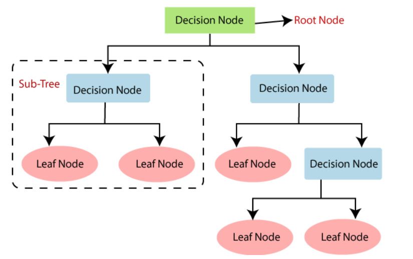
Risks 2021, 9, 42                                                                                                               2 of 23

                                     efficient method to determine the risk a driver poses to insurance companies. Thus, these
                                     companies will adjust the insurance prices fairly to a driver’s ability and relevant personal
                                     information, making automotive insurance more accessible to clients. The forecast for
                                     claims occurrence will support the modification of insurance quotes based on the client’s
                                     ability. If a client has a good driving record, it would be unreasonable for a client with a
                                     poor driving background to pay a similar insurance premium. Therefore, the model should
                                     show which clients are unlikely to make claims, decrease their insurance cost, and raise the
                                     insurance cost for those who are likely to make a claim. Thus, more insurance companies
                                     want to have an insurance premium that is appropriate for each customer. This kind of
                                     premium is very relevant in regulatory and business terms. For the regulatory level, it is
                                     the best way to avoid discrimination and provide fair prices, and, for the business level, it
                                     gives calculations with flexibility, simplicity, and precision, allowing them to respond to
                                     any circumstance and control any loss.
                                           According to the Insurance Information Institute report, the claims frequency, amount
                                     of claims per car, and claim severity are on the rise, e.g., accident claim severity increased by
                                     35% for US car insurance between 2010 and 2019. The average US car insurance expenditure
                                     increased from USD $78,665 in 2009 to USD $100,458 in 20172 . This increase indicates that
                                     a quicker and more efficient system for filing auto insurance claims is needed to follow the
                                     growing trends in claim severity and frequency. These facts make auto insurance pricing
                                     studies more meaningful and essential.
                                           In the insurance industry, it is essential to set the product’s price before knowing its
                                     cost. This reality makes the process of rate-making more critical and significant. Insurance
                                     firms must predict how many claims are going to occur and the severity of these claims to
                                     enable insurers to set a fair price for their insurance products accordingly. In other words,
                                     claim prediction in the auto insurance sector is the cornerstone of premium estimates.
                                     Furthermore, it is crucial in the insurance sector to plan the correct insurance policy for each
                                     prospective policyholder. Failure to foresee auto insurance claims with accuracy would
                                     raise the insurance policy’s cost for the excellent client and lower the bad client’s price of the
                                     policy. This is referred to as pay-as-you-drive, and this strategy is an alternate mechanism
                                     for pricing premiums based on the customer’s personal driving behavior. The importance
                                     of pay-as-you-drive insurance policies was highlighted by Hultkrantz et al. (2012), as they
                                     enable the insurers to personalize the insurance costs for each client, thus the premium
                                     rate will be fair. Several studies have been done to personalize the premium estimate, such
                                     as Guillen et al. (2019) and Roel et al. (2017), they demonstrated the possible benefits of
                                     analyzing information from telematics when determining premiums for auto insurance.
                                     The predictive capacity of covariates obtained from telematics vehicle driving data was
                                     investigated by Gao and Wüthrich (2018) and Gao et al. (2019) using the speed–acceleration
                                     heatmaps suggested by Wüthrich (2017).
                                           Prediction accuracy enables the insurance industry to adjust its premiums better, and
                                     makes car insurance coverage more affordable for more drivers. Currently, many insurance
                                     companies are using ML methods instead of a conventional approach, which offers a
                                     more comprehensive way of producing a more reliable and representative outcome. A
                                     new study related to artificial intelligence and business profit margins was conducted
                                     by McKinsey & Company (Columbus 2017). They showed that the businesses that have
                                     completely embraced artificial intelligence projects have generated a higher profit margin
                                     of 3% to 15%. However, selecting a suitable ML predictive model has yet to be fully
                                     addressed. In this study, we investigate more powerful ML techniques to make an accurate
                                     prediction for claims occurrence by analyzing the big dataset given by Porto Seguro, a large
                                     automotive company based in Brazil3 , and we apply the ML methods in the dataset, such
                                     as logistic regression, XGBoost, random forest, decision trees, naïve Bayes, and K-NN. We
                                     also evaluate and compare the performance of these models.

2   https://www.iii.org/fact-statistic/facts-statistics-auto-insurance (accessed on 19 December 2020).
3   https://www.kaggle.com/alinecristini/atividade2portoseguro (accessed on 15 December 2020).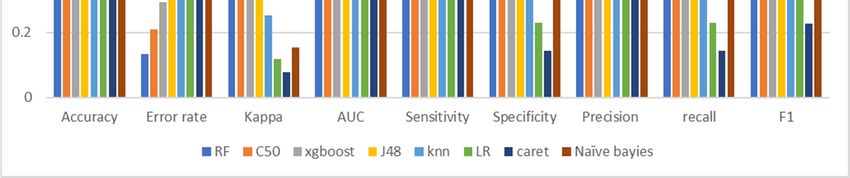
Risks 2021, 9, 42                                                                                          3 of 23

                         This paper’s main objective is to create an ML algorithm that accurately predicts
                    claims occurrence. Thus, the model must effectively consider consumer details, such as
                    the type of vehicle or the car’s cost, that differ among the clients. The model’s results
                    (and provided that the forecast is accurate) confirmed that car insurance firms will make
                    insurance coverage more available to more clients.

                    2. Related Work
                         There is a lot of motivation for automotive insurance companies to implement machine
                    learning algorithms in their business, as they are used for driver performance monitoring
                    and insurance market analytics. Several papers have discussed the issue of prediction in
                    the insurance sector by using ML models, such as Smith et al. (2000), who tested several
                    machine learning models, like the decision tree and neural networks, to assess whether the
                    policyholder submits a claim or not and addressed the effect that the case study will have
                    on the insurance company. Weerasinghe and Wijegunasekara (2016) compared three ML
                    methods for predicting claims severity. Their findings showed that the best predictor was
                    the neural networks. Another example of a similar and satisfactory solution to the same
                    problem is the thesis “Research on Probability-based Learning Application on Car Insur-
                    ance Data” (Jing et al. 2018). They used only a Bayesian network to classify either a claim
                    or no claim, and Kowshalya and Nandhini (2018), in order to predict fraudulent claims
                    and calculate insurance premium amounts for various clients according to their personal
                    information, used ML techniques; three classifiers were used to predict fraudulent claims,
                    and these classifiers were random forest, J48, and naïve Bayes algorithms. The findings
                    indicated that random forests outperform the remaining techniques. This paper does not
                    involve forecasting insurance claims, but focuses on fraudulent claims. Additionally, an
                    example of insurance market analytics is a model that predicts claim severity virtually,
                    as well as the funds needed to repair vehicle damage (Dewi et al. 2019). This example
                    represents how insurance providers look into many different forms of applying machine
                    learning to their customer data. In the work that proposed a system (Singh et al. 2019), this
                    system takes photos of the damaged vehicle as inputs. It generates specific information,
                    such as the cost of repair used, to determine an insurance claim’s cost. Therefore, this
                    paper does not involve the prediction of insurance claims occurrence, but was focused on
                    estimating the repair cost (Stucki 2019). This study aims to provide an accurate method
                    for insurance companies to predict whether the customer relationship with the insurer
                    will be renewed or not after the first period that the consumer acquires new insurance,
                    such as a vehicle, life, or property insurance; this study forecasts the potential turnover
                    of the customer, and five classifiers were used. These classifiers are algorithms for LR, RF,
                    KNN, AB, and ANN. This study showed that the best performing model was random
                    forests. Pesantez-Narvaez et al. (2019) use two competing methods, XGBoost and logistic
                    regression, to predict the frequency of motor insurance claims. This study shows that the
                    XGBoost model is slightly better than logistic regression; however, they used a database
                    comprised of only 2767 observations. Furthermore, a model for predicting insurance
                    claims was developed (Abdelhadi et al. 2020); they built four classifiers to predict the
                    claims, including XGBoost, J48, ANN, and naïve Bayes algorithms. The XGBoost model
                    performed the best among the four models, and they used a database comprised of 30,240
                    observations.
                         All of the above studies considered neither big volume nor missing value issues.
                    Therefore, in this paper, we focus on examining the machine learning methods that are
                    the most suitable method for claim prediction with big training data and many missing
                    values. Therefore, this study will have more variety in combining models for an accurate
                    claim prediction, looking for the alternative and more complex machine learning model
                    to predict the probability of claims occurring in the next year by using a real database
                    provided by Porto Seguro company. Furthermore, from the above studies, we can say that
                    some of the previous recent studies that applied some machine learning models in the
                    insurance industry show that the XGBoost model is the best model for classification in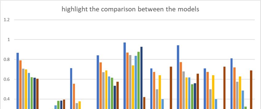
Risks 2021, 9, 42                                                                                                                   4 of 23

                                   the insurance industry (Pesantez-Narvaez et al. 2019; Abdelhadi et al. 2020). They used a
                                   database comprised of 2767 and 30,240 observations, respectively, while (Jing et al. 2018)
                                   shows that the naïve Bayes is an effective model for claims occurrence prediction. In our
                                   paper, we use big data that contained almost a million and a half (1,488,028) observations
                                   with 59 variables, and our results show that XGBoost is a useful model. Still, our results
                                   also show that RF and the decision tree (C50) is significantly better than XGBoost. Our
                                   results also show that the naïve Bayes is the worst model for predicting claims occurrence
                                   among all eight classification models used in this study. On the other hand, our results are
                                   consistent with a recent study (Dewi et al. 2019). The difference between this study and our
                                   study is that our study focuses on predicting the probability of claim occurrence, compared
                                   to predicting the cost of a claim and the funds required for the claim damage when the
                                   claim occurred. Their results are consistent with ours, showing that the random forest has
                                   the higher accuracy, and can be applied whether in cases of prediction of claim severity,
                                   as the results of their study shows, or in claim occurrence prediction, as our study shows.
                                   These results confirm the scalability of the random forest. Hence, the random forest model
                                   can be used to solve big data problems related to data volume. The results of the literature
                                   review have been summarized in Table 1.

                Table 1. Different studies for using ML models in the insurance industry to get a representative overview.

                                                                                                      Performance            The Best
 ARTICLE & YEAR                            PURPOSE                            Algorithms
                                                                                                        Metrics               Model
                                Classification to predict customer                                      Accuracy
 (Smith et al. 2000)                                                            DT, NN                                         NN
                                        retention patterns                                               ROC
                               Classification to predict the risk of
 (Günther et al. 2014)                                                       LR and GAMS                  ROC                  LR
                                             leaving
                                                                                                        Precision
 (Weerasinghe and             Classification to predict the number
                                                                              LR, DT, NN                  Recall               NN
 Wijegunasekara 2016)             of claims (low, fair, or high)
                                                                                                        Specificity
                                Regression to forecast insurance                                        R-squares
 (Fang et al. 2016)                                                     RF, LR, DT, SVM, GBM                                   RF
                                    customer profitability                                               RMSE
                                                                                                        Sensitivity
 (Subudhi and                  Classification to predict insurance
                                                                            DT, SVM, MLP                Specificity           SVM
 Panigrahi 2017)                              fraud
                                                                                                        Accuracy
                                                                                                        Accuracy
                                 Classification to predict churn,                                         AUC
 (Mau et al. 2018)                                                                 RF                                          RF
                                  retention, and cross-selling                                            ROC
                                                                                                         F-score
                                                                                                                       Both have the
                                 Classification to predict claims        Naïve Bayes, Bayesian,
 (Jing et al. 2018)                                                                                     Accuracy           same
                                            occurrence                      Network model
                                                                                                                         accuracy.
                               Classification to predict insurance                                      Accuracy
 (Kowshalya and
                               fraud and percentage of premium            J48, RF, Naïve Bayes          Precision              RF
 Nandhini 2018)
                                             amount                                                      Recall
                                                                        RF, AB, MLP, SGB, SVM,
                                 Classification to predict churn
 (Sabbeh 2018)                                                         KNN, CART, Naïve Bayes,          Accuracy               AB
                                             problem
                                                                               LR, LDA.
                                                                                                        Accuracy
                               Classification to predict churn and
 (Stucki 2019)                                                         LR, RF, KNN, AB, and NN           F-Score               RF
                                            retention
                                                                                                          AUC
 (Dewi et al. 2019)           Regression to predict claims severity          Random forest                MSE                  RF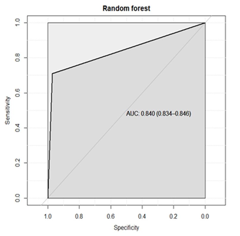
Risks 2021, 9, 42                                                                                                               5 of 23

                                                               Table 1. Cont.

                                                                                                        Performance       The Best
    ARTICLE & YEAR                         PURPOSE                              Algorithms
                                                                                                          Metrics          Model
                                                                                                            Sensitivity
                                                                                                            Specificity
    (Pesantez-Narvaez            Classification to predict claims
                                                                                XGBoost, LR                 Accuracy      XGBoost
    et al. 2019)                            occurrence
                                                                                                              RMSE
                                                                                                              ROC
                                 Classification to predict claims                                           Accuracy
    (Abdelhadi et al. 2020)                                            J48, NN, XGBoost, naïve base                       XGBoost
                                            occurrence                                                       ROC

                                         Table 1 is a chronological table that shows different studies for using ML models in the
                                    insurance industry, where LR is a logistic regression model, GAMS is a generalized additive
                                    model, RF is a random forest model, KNN is a K-nearest neighbor model, NN is a neural
                                    network model, DT is a decision tree, AB is an AdaBoost model, MLP is a multi-layer
                                    perceptron model, SGB is a stochastic gradient boosting model, SVM is a support vector
                                    machine model, MSE is the mean square error, and RMSE is the root mean square error.

                                    3. Background
                                         To understand the problem, it is essential to understand the insurance claims forecast,
                                    big data, ML, and classification. We explore the following terms.
                                         The vast amount of data to determine the probability of claims occurrence makes
                                    a claim prediction issue require big data models. Thus, there is a need for an effective
                                    approach and a more reliable ML model to assess the danger that the driver poses to the
                                    insurance provider and the probability of filing a claim in the coming year, a model that
                                    can read and interpret vast databases containing thousands of consumer details provided
                                    by the Porto Seguro insurance company.
                                         Porto Seguro is one of the biggest car and homeowner insurance firms in Brazil. Porto
                                    Seguro claims that their automotive division’s mission is to customize insurance quotes
                                    based on the driver’s ability. They believe that effective techniques can be applied for more
                                    accurate results to predict claims occurrence in the coming year. Thus, they provided the
                                    dataset containing 59 variables with 1,488,028 observations4 . These observations include
                                    customer information that the company collected over several years.

                                    3.1. Machine Learning
                                          Machine learning is an area of computer science research that is gradually being
                                    adopted in data analysis, and it has gained high demand in the last decade (Géron 2019).
                                    Its rapid dissemination is due to the rapid growth of data generated from many sources
                                    and the vast quantities of data stored in databases. It enables individuals and organizations
                                    to understand their datasets in more detail. Forbes’s research has also indicated that
                                    one in ten companies now uses ten or more AI applications: 21% of the applications
                                    are based on fraud detection, 26% on process optimization, and 12% on opinion mining
                                    (Columbus 2018). Machine learning extends artificial intelligence, and can help machines
                                    develop their expertise by learning from the data and defining models with the minimum
                                    human involvement, and, through logic and conditions, a prediction can be made using
                                    learning algorithms (Goodfellow et al. 2016).
                                          There is a significant number of applications for machine learning in industries avail-
                                    able, including predictive models for online shopping, fraud detection in banks, or even
                                    spam filtering in email inboxes (Schmidt et al. 2019). However, the underlying principle
                                    behind these implementations is that the model must generalize well to generate reliable
                                    forecasts (Gonçalves et al. 2012). Machine learning aims primarily to discover models and

4    https://www.kaggle.com/c/porto-seguro-safe-driverprediction/overview (accessed on 15 December 2020).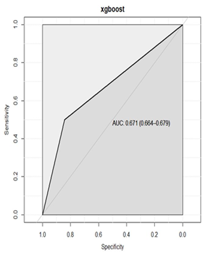
Risks 2021, 9, 42                                                                                              6 of 23

                    patterns in data and use them to predict future outcomes (D’Angelo et al. 2017). One of
                    the key aims of most research in artificial intelligence (AI) and big data analytics areas
                    is learning complex trends, features, and relationships from vast data volumes. The ba-
                    sis for the application of AI in information discovery applications is machine learning
                    and data mining based approaches. The essence of the intelligent machine’s learning
                    method is the comparison between the objective to be achieved and the result derived
                    by the machine state. In many research fields, this method has proved to be successful
                    (D’Angelo et al. 2020), including in analysis of the insurance industry (Jing et al. 2018;
                    Pesantez-Narvaez et al. 2019; Dewi et al. 2019; Abdelhadi et al. 2020). The generic machine
                    learning algorithm will receive input data and split this data into two sets, the first called
                    the training and the second called the test dataset. The model trained through training
                    data is set to make predictions and determine the model’s ability to generalize to external
                    data. The model evaluates the test data to determine if it predicts correctly.

                    3.2. Machine Learning Approach to Predict a Driver’s Risk
                         The prediction of the claims is intended to predict it the insured will file a claim or
                    not. Let Y = {0,1} be the output possible, with 0,1 being categorical values that reflect that
                    the client ‘will not file a claim’ or ‘will file a claim’, respectively.
                         The purpose of this machine learning model is to predict the probability of claim
                    occurrence. This algorithm is modeled on data representing a customer that has (a) made
                    a claim or (b) not made a claim. Therefore, the problem can be identified as a binary
                    classification, where a claim is a 1 and no claim made is a 0 (Kotsiantis et al. 2006). Different
                    classification algorithms can be used. Some of them perform better, and others perform
                    worse, given the data state (Kotsiantis et al. 2007).

                                                            Pr(Y = 0|X = xi),                                     (1)

                                                             Pr(Y = 1|X = xi)                                     (2)
                    where X is a collection of instances xi that represents all of the known information of the
                    i-th policyholder.

                    3.3. Classifiers
                    3.3.1. Regression Analysis
                          Linear regression is used to estimate the linear relationship between a variable of
                    response (target) and a set of predictor variables. However, linear regression is not suitable
                    when the target variable is binary (Sabbeh 2018). For the binary-dependent variables,
                    logistic regression (LR) is a suitable model for evaluating regression. LR is a statistical
                    analysis used to describe how a binary target variable is connected to various independent
                    features. It has many similarities with linear regression.
                          LR is a multivariable learning algorithm for dichotomous results. It is a classification
                    method with the best performance for models with two outputs, e.g., yes/no decision-
                    making (Musa 2013). Therefore, it is suitable for predicting a vehicle insurance claim with
                    two variables (claim or no claim). LR is similar to linear regression by its functionality.
                    However, linear regression provides a continuous output compared to the categorical
                    output we desire in the binary target variable. LR performs with a single output variable,
                    yi , where i = {1, ... n}, and each yi can hold one of two values, 0 or 1 (but not both). This
                    follows the Bernoulli probability density function, as in the following equation:

                                                      p ( y i ) = ( π i ) y i (1 − π i )1− y i                    (3)

                         This takes the value 1 when the probability is πi , and 0 when the probability is 1 − πi ;
                    the interest in this is when yi = 1 with an interesting probability πi . The classifier will then
Risks 2021, 9, 42 7 of 23
produce the output of the predicted label; πi is equal to 1 if it is greater than or equal to its
threshold (by default, 0.5) (Musa 2013).
Risks 2021, 9, x FOR PEER REVIEW i f ( p(y = 1)) ≥ the instance ∈ class(y = 1) 7 of (4)
23
i f ( p(y = 1)) < the instance ∈ class(y = 1) (5)
3.3.2.
3.3.2.Decision
DecisionTree
Tree
AAdecision
decisiontree
treeisis aa supervised
supervised learning
learning approach
approachused used toto solve
solve classification
classification andand
regression
regressionissues,
issues,butbutit is
it mostly used
is mostly usedto solve classification
to solve issues.
classification It is a Itclassifier
issues. orga-
is a classifier
nized by the
organized bytree
the structure,
tree structure,where
wherethe the
internal nodes
internal nodesareare
thethe
data
datavariables,
variables,the thebranches
branches
are
arethethedecision
decision rules,
rules, and each nodenode isis the
the output.
output.ItItconsists
consistsofoftwo
twonodes.
nodes.One Oneofofthem
themis
isa adecision
decisionnode
nodeusedusedforfordecision-making,
decision-making,and anditithas
hasvarious
variousbranches.
branches.TheThesecond
secondnode
nodeis
isa aleaf
leafnode,
node,which
whichrepresents
representsthe theresult
resultofofthese
thesedecisions.
decisions.
Decision
Decisiontrees
treesprovide
providemany manyadvantages,
advantages,but butusually
usuallydo donot
not perform
perform predictively
predictively
compared
comparedtotomore morecomplex
complexalgorithms.
algorithms.However,
However,therethereare
arestrong
strongensemble
ensemblealgorithms,
algorithms,
such
suchas asrandom
randomforests
forests and gradient boosters,
boosters,thatthatare
aredeveloped
developedintelligently
intelligentlybybycombining
combin-
ing several
several decision
decision trees.
trees. ThereThere
are are
alsoalso different
different DTs DTs models:
models: CART, CART,
C4.5,C4.5,
C5.0,C5.0, and
and more
more
(Song(Song and Ying
and Ying 2015).2015).
Figure11shows
Figure showsthethestructure
structureofofaageneral
generaldecision
decisiontree.
tree.
Structureofofaageneral
Figure1.1.Structure
Figure generaldecision
decisiontree.
tree.
3.3.3. XGBoost
3.3.3. XGBoost
XGBoost is a novel approach proposed by Chen and Guestrin to raise the gradient tree
XGBoost is a novel approach proposed by Chen and Guestrin to raise the gradient
(Chen and Guestrin 2016). It uses various decision trees to predict a result. Figure 2 shows
tree (Chen and Guestrin 2016). It uses various decision trees to predict a result. Figure 2
the methodology of the XGBoost model. XGBoost stands for extreme gradient boosting.
shows the methodology of the XGBoost model. XGBoost stands for extreme gradient
A regression and classification problem learning technique optimizes a series of weak
boosting. A regression and classification problem learning technique optimizes a series of
prediction models to construct a precise and accurate predictor. It is a desirable model,
weak prediction models to construct a precise and accurate predictor. It is a desirable
because it can boost weak learners (Zhou 2012). Furthermore, it can improve the insurance
model, because it can boost weak learners (Zhou 2012). Furthermore, it can improve the
risk classifier’s performance by combining multiple models. Some studies showed that
insurance risk classifier’s performance by combining multiple models. Some studies
the XGBoost model is the best model for the prediction of claims occurrence with a small
showed that the XGBoost model is the best model for the prediction of claims occurrence
dataset (Pesantez-Narvaez et al. 2019).
with a small dataset (Pesantez-Narvaez et al. 2019).
Figure 2. XGBoost methodology.boosting. A regression and classification problem learning technique optimizes a series of
weak prediction models to construct a precise and accurate predictor. It is a desirable
model, because it can boost weak learners (Zhou 2012). Furthermore, it can improve the
insurance risk classifier’s performance by combining multiple models. Some studies
showed that the XGBoost model is the best model for the prediction of claims occurrence
Risks 2021, 9, 42 8 of 23
with a small dataset (Pesantez-Narvaez et al. 2019).
Figure 2. XGBoost methodology.
Figure 2. XGBoost methodology.
3.3.4. Random Forest
Random forests reflect a shift to the bagged decision trees that create a broad number
of de-correlated trees so that predictive efficiency can be improved further. They are a
very popular “off-the-box” or “off-the-shelf” learning algorithm with good predictive
performance and relatively few hyper-parameters. There are many random forest imple-
mentations, however, the Leo Breiman algorithm (Breiman 2001) is widely authoritative.
Random forests create a predictive value as a result of the regression of individual trees. It
resolves to over-fit (Kayri et al. 2017). A random forest model can be expressed as follows:
g( x ) = f 0 ( x ) + f 1 ( x ) + f 2 ( x ) + . . . + f n ( x ) (6)
where g is the final model, i.e., the sum of all models. Each model f (x) is a decision tree.
3.3.5. K-Nearest Neighbor
K-nearest neighbor is based on supervised learning techniques. It is considered one
of the most straightforward ML models. K-NN assumes the comparison between the
available data and the new data; it includes the new data in the category nearest to the
classes available. It can be used for classification regression, but it is mainly used for
classification. It is also known as a lazy model (Cunningham and Delany 2020), since it
does not learn from the training dataset instantly. K-NN modes only store the dataset
through training; when K-NN receives new data, it classifies this new data to the nearest
available category based on the training data stored in the K-NN model. It can also be
inefficient computationally. However, K-NNs have succeeded in several market problems
(Mccord and Chuah 2011; Jiang et al. 2012).
3.3.6. Naïve Bayes
Naïve Bayes shows that the naïve Bayesian network can have good predictive performance
compared to other classifiers, such as neural networks or decision trees (Friedman et al. 1997).
From the training data, naïve Bayes classifiers learn each attribute Ai’s conditional prob-
ability on the class label C. For classification, the Bayes rule is applied to calculate the
probability of C on the attribute instance Ai, . . . , An. The class that will be predicted
is the class with the highest probability. For feasibility, the classifier operates under the
assumption that all attributes Ai are conditionally independent given the value of class C.
Figure 3 shows the methodology of the Naïve Bayes model.
Because all attributes are processed independently, the performance can be surprising.
This is because it ignores potentially significant correlations between features.man et al. 1997). From the training data, naïve Bayes classifiers learn each attribute Ai’s
conditional probability on the class label C. For classification, the Bayes rule is applied to
calculate the probability of C on the attribute instance Ai, …, An. The class that will be
predicted is the class with the highest probability. For feasibility, the classifier operates
under the assumption that all attributes Ai are conditionally independent given the value
Risks 2021, 9, 42 9 of 23
of class C. Figure 3 shows the methodology of the Naïve Bayes model.
Figure 3. Naïve Bayes network structure.
Figure 3. Naïve Bayes network structure.
4. Evaluation Models (Prediction Performance)
There are
Because allseveral metrics
attributes to evaluate
are processed a classifier model
independently, and examine
the performance how
can well the
be surpris-
ing. This is because it ignores potentially significant correlations between features. 2015).
model fits a dataset and its performance on the unseen data (Hossin and Sulaiman
Accuracy alone for a classification problem cannot always be reliable, because it can
4.provide
Evaluation Models
bias for (Prediction
a majority Performance)
class giving high accuracy and weak accuracy for the minority
class, making it less informative for predictions,
There are several metrics to evaluate a classifier especially
modelin and
the case of imbalanced
examine how well data
the
(Ganganwar 2012). Car insurance claims are an excellent example of imbalanced
model fits a dataset and its performance on the unseen data (Hossin and Sulaiman 2015). data,
because the majority of policyholders do not make a claim. Therefore, if accuracy is used,
there would be a bias toward a no claim class. Thus, we use other measures, such as kappa,
F-measure, and the area under the curve (AUC). To understand how accuracy works, it is
important to understand firstly how a confusion matrix works.
4.1. Confusion Matrix
A confusion matrix is used for binary classification problems. It is a beneficial method
to distinguish which class outputs were predicted correctly or not. As shown in Table 2, the
rows represent the predicted class, while the columns represent the actual class (Hossin and
Sulaiman 2015). In the matrix, TP and TN represent the quantity of correctly classified
positive and negative instances, whereas FP and FN represent incorrectly classified positive
and negative samples, respectively.
Table 2. Confusion matrix.
Actual Positive Actual Negative
Predicted positive True positive (TP) False negative(FN)
Predicted negative False positive (FP) True negative (TN)
In car insurance claims, true positive would represent no claim made, and true
negative would represent a claim.
TP + TN
Accuracy = (7)
( TP + FP + TN + FN )
4.2. Kappa Statistics
Kappa statistics significantly measure besides the accuracy, because it considers the
probability of a correct prediction in both classes 0 and 1. Kappa is essential for datasets
with extreme class imbalance, such as auto insurance claims, since a classifier can achieve
high precision by merely guessing the most common class.
pr ( a) − pr (e)
K= (8)
1 − pr (e)Risks 2021, 9, 42 10 of 23
4.3. Sensitivity and Specificity
The sensitivity (true positive rate) evaluates the ratio of positive classified examples
correctly by comparing the predicted positive class with the actual positive, while the
specificity (true negative rate) evaluates the ratio of negative classified examples correctly
by comparing the predicted negative class with the actual negative.
Sensitivity = TP/( TP + FN ) (9)
Speci f ity = TN/( FP + TN ) (10)
4.4. Precision and Recall
The precision metric is used to measure how trustworthy the class is classified, and if
it belongs to the right class. Another useful metric is recall, which is used to measure how
well the fraction of a positive class becomes correctly classified; this essentially shows how
well the model can detect the class type (Hossin and Sulaiman 2015).
TP
Precision = (11)
TP + FP
TP
recall = (12)
TP + FN
4.5. The F-Measure
The F-measure is a measure of model performance that combines precision and recall
into a single number known as the F-measure (also called the F1 score or the F-score). The
following is the formula for the F-measure:
2 ∗ precision × recall 2 × TP
F − measure = (13)
recall + precision 2 × TP + FP + FN
Additionally, the area under the receiver operator characteristics (ROC) curve (AUC)
is needed, since there is a weakness in accuracy, precision, and recall, because they are not
as robust to the change of class distribution; a popularly used ranking evaluation technique
is to use the AUC metric, otherwise known as the receiver operating characteristic (ROC)
or the global classifier performance metric, since all different classification schemes are
measured to compare overall performance (Wu and Flach 2005). If the test set were to
change its distribution of positive and negative instances, the previous metrics might
not perform as well as when they were previously tested. However, the ROC curve is
insensitive to the change in the proportion of positive and negative instances and class
distribution (Bradley 1997).
5. Dataset
In this study, we analyze a dataset given by Porto Seguro, a large Brazilian automotive
company. Due to the privacy of this dataset, the database is kept safe and confidential, and
the clients’ personal information is encrypted5 . Some data, like categorical data, can be
found in dataset columns. For example, ps car 04 cat may provide a general indication of
planned car data (e.g., car type or car use), but for protective purposes, it is not specified.
It is necessary to understand how the datasets were structured before changing the
dataset to construct the ML model. Our set of big data consists of 59 variables and 1,488,028
rows, and every row contains the personal details of a different single client. A data
description has also been issued that contains essential data on the already processed data
preparation. The key points to be noted are:
• Values of −1 indicate that the feature was missing from the observation.
5 https://www.kaggle.com/c/porto-seguro-safe-driver-prediction/data (accessed on 15 December 2020).Risks 2021, 9, 42 11 of 23
• Feature names include the bin for binary features and cat for categorical features.
# Binary data has two possible values, 0 or 1.
# Categorical data (one of many possible values) have been processed into a
value range for its lowest and highest value, respectively.
• Features are either continuous or ordinal.
# The value range appears as a range that has used feature scaling; therefore,
feature scaling is not required.
• Features belonging to similar groupings are tagged as ind, reg, car, and calc.
# ind refers to a customer’s personal information, such as their name.
# reg refers to a customer’s region or location information.
Risks 2021, 9, x FOR PEER REVIEW 11 of 23
# calc is Porto Seguro’s calculated features.
6. Proposed Model
6. Proposed
In thisModel
paper, we developed a model to predict the occurrence of car insurance claims
byInapplying MLwe
this paper, techniques.
developed And the to
a model stages of the
predict preparing the of
occurrence proposed model
car insurance shown
claims by in
Figure ML
applying 4. techniques. And the stages of preparing the proposed model shown in Figure 4.
Figure
Figure 4. Overall
4. Overall structure
structure of the
of the proposed
proposed model.
model.
6.1.6.1. Data
Data Preprocessing
Preprocessing
The
The dataset
dataset consists
consists of of
5959 variables.
variables. Each
Each of of these
these attributes
attributes hashas
itsits relation
relation to to
thethe
insurance claims occurrence, which is our dependent target variable. The data is checked
insurance claims occurrence, which is our dependent target variable. The data is checked
and modified to apply the data to the ML algorithms efficiently. We begin by considering
and modified to apply the data to the ML algorithms efficiently. We begin by considering
the variable answer (dependent), target, then, all missing values are cleaned, as we shall
the variable answer (dependent), target, then, all missing values are cleaned, as we shall
see in Sections 6.1.1 and 6.1.2.
see in Sections 6.1.1 and 6.1.2.
6.1.1. Claims Occurrence Variable
6.1.1. Claims Occurrence Variable
Our target column is a binary variable that contains two classes (1,0), 1 if a claim has
Our target
occurred and column is a binary
a 0 if a claim variable
has not thatFigure
occurred. contains two classes
5 shows (1,0), 1 if aofclaim
the distribution 1 andhas
0 for
occurred and a 0 if
the target column. a claim has not occurred. Figure 5 shows the distribution of 1 and 0 for
the target column.the variable answer (dependent), target, then, all missing values are cleaned, as we shall
see in Sections 6.1.1 and 6.1.2.
6.1.1. Claims Occurrence Variable
Risks 2021, 9, 42 Our target column is a binary variable that contains two classes (1,0), 1 if a claim
12 ofhas
23
occurred and a 0 if a claim has not occurred. Figure 5 shows the distribution of 1 and 0 for
the target column.
Risks 2021, 9, x FOR PEER REVIEW 12 of 23
Figure 5.
Figure 5. Histogram of the
the distribution
distribution of
of target
target values.
values.
The
The figure
figure shows
shows that
that the
the target
target variable
variable is heavily imbalanced,
is heavily imbalanced, with with class
class 00 having
having
0.963% observations and class 1 having only 0.037%
0.963% observations and class 1 having only 0.037% observations. observations.
An
An algorithm
algorithmfor forML
MLdoesdoesnotnotperform
perform efficiently
efficiently forfor
imbalanced
imbalanced data. Thus,
data. we ap-
Thus, we
plied
appliedthethe
oversampling.
oversampling. Oversampling
Oversampling means that that
means therethere
are more representations
are more representationsof class
of
1, so the
class 1, soprobability of class
the probability 1 increases.
of class Figure
1 increases. 6 represents
Figure a binary
6 represents target
a binary variable
target dis-
variable
tribution after
distribution applying
after a random
applying a random oversample
oversample using thethe
using ROSE library.
ROSE library.
We
We balanced the given data using the function ROSE from a library called ROSE. The
ROSE
ROSE package is an an RR package.
package.In Inthe
thepresence
presenceofofimbalanced
imbalancedclasses,
classes,it it offers
offers functions
functions to
to deal
deal with
with binary
binary classification
classification issues.
issues. According
According to ROSE,
to ROSE, synthetic
synthetic balanced
balanced samples
samples are
produced
are produced (Lunardon
(Lunardonet al.et2014). Functions
al. 2014). are also
Functions givengiven
are also that apply moremore
that apply conventional
conven-
remedies
tional to the class
remedies to theimbalance. Balanced
class imbalance. samplessamples
Balanced are generated by random
are generated oversampling
by random over-
of minority
sampling ofexamples, under-sampling
minority examples, of majority of
under-sampling examples,
majorityorexamples,
over- andor under-sampling
over- and un-
combinations.combinations.
der-sampling
Figure
Figure 6.
6. Histogram
Histogram of the balanced distribution of
of target
target values
values after
afterusing
usingthe
theROSE
ROSEpackage
packageininR.
R.
6.1.2. Details on Missing Values
Before presenting our analysis, we will briefly examine different combinations of
missing values in the data. In the following plot, the frequency of missing values per fea-
ture is shown in the top bar plot. Thus, the more red rectangles a feature has, the moreRisks 2021, 9, 42 13 of 23
6.1.2. Details on Missing Values
Before presenting our analysis, we will briefly examine different combinations of
missing values in the data. In the following plot, the frequency of missing values per
feature is shown in the top bar plot. Thus, the more red rectangles a feature has, the more
missing values.
As shown in Figures 7 and 8, we obtain:
• The features of ps_car_03_cat and ps_car_05_cat have the largest number of missing
values. They also share numerous instances where missing values occur in both for
the same row.
• Some features share many missing value rows with other features, for instance,
ps_reg_03. Other features have few missing values, like ps_car_12, ps_car_11, and
ps_car_02.cat.
• We find that about 2.4% of the values are missing in total in each of the train and test
Risks 2021, 9, x FOR PEER REVIEW datasets. 13 of 23
• From this figure, the features have a large proportion of missing values, being roughly
70% for ps_car_03_cat and 45% for ps_car_05_cat; therefore, these features are not that
reliable,
may alsoas there
not are too
convey thefew valuespurpose
feature’s to represent
and the feature’simpact
negatively true meaning. Assigning
the learning algo-
new values that are missing to each customer record for these features may also
rithm’s performance. Due to these reasons, the features have been dropped and re-
not convey the feature’s purpose and negatively impact the learning algorithm’s
moved from the datasets.
performance. Due to these reasons, the features have been dropped and removed
• After we drop ps_car_03_cat and ps_car_05_cat, the features missing values in da-
from the datasets.
tasets become 0.18 instead of 2.4. The missing values for the rest of the variables are
• After we drop ps_car_03_cat and ps_car_05_cat, the features missing values in datasets
replaced such that missing values in every categorical and binary variable are re-
become 0.18 instead of 2.4. The missing values for the rest of the variables are replaced
placed by the mode of the column values. In contrast, missing values in every con-
such that missing values in every categorical and binary variable are replaced by the
tinuous variable are replaced by the mean of the column values. This is because cat-
mode of the column values. In contrast, missing values in every continuous variable
egorical data works well using the mode, and continuous data works well using the
are replaced by the mean of the column values. This is because categorical data works
mean. Both methods are also quick and straightforward for inputting values (Badr
well using the mode, and continuous data works well using the mean. Both methods
2019).
are also quick and straightforward for inputting values (Badr 2019).
Figure
Figure7.7.Missing
Missingvalues
valuesin
inour
ourdata.
data.Risks 2021, 9, 42 14 of 23
Figure 7. Missing values in our data.
Risks 2021, 9, x FOR PEER REVIEW 14 of 23
Figure8.8.Missing
Figure Missingvalues
valuesin
inour
ourdata.
data.
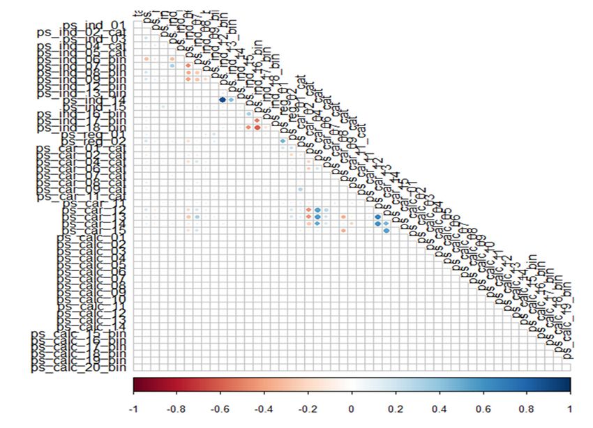
6.1.3. Correlation Overview
6.1.3. Correlation Overview
As As
previously
previouslyshown,
shown,somesomefeature selections
feature have
selections have been processed,
been processed,eliminating
eliminatingthethe
ps ps
carcar
03 03
catcat
andand
ps ps
carcar
05 05
catcat
features, because
features, becausethey
theyhadhad tootoo
many
many missing
missingvalues, andand
values,
they
they willwill
notnot be useful
be useful to algorithm.
to an an algorithm. At this
At this point,
point, it isitessential
is essential to visualize
to visualize andand classify
classify
thethe features
features thatthat
areare more
more useful
useful using
using thethe Pearson
Pearson correlation
correlation coefficient,
coefficient, as as shown
shown in in
Figure
Figure 9. 9.
Figure
Figure 9. Correlation
9. Correlation matrix
matrix of data
of all all data features.
features.
These results showed that all calc variables do not correlate well with other variables.
These results showed that all calc variables do not correlate well with other variables.
Despite other features with a relatively poor relationship with the target variable, the
Despite other features with a relatively poor relationship with the target variable, the calc
calc variables do not correlate with the target variable. This is important, since the target
variables do not correlate with the target variable. This is important, since the target var-
variable dictates whether a claim occurs or not, so a specific correlation may occur. Due to
iable dictates whether a claim occurs or not, so a specific correlation may occur. Due to
this, the calc features for the datasets are dropped. We conducted a Pearson correlation, but
this, the calc features for the datasets are dropped. We conducted a Pearson correlation,
did so after removing calc features; Figure 10 shows the Correlation matrix of data features
but did so after removing calc features; Figure 10 shows the Correlation matrix of data
after we drop calc features.
features after we drop calc features.These results showed that all calc variables do not correlate well with other variables.
Despite other features with a relatively poor relationship with the target variable, the calc
variables do not correlate with the target variable. This is important, since the target var-
iable dictates whether a claim occurs or not, so a specific correlation may occur. Due to
Risks 2021, 9, 42 this, the calc features for the datasets are dropped. We conducted a Pearson correlation, 15 of 23
but did so after removing calc features; Figure 10 shows the Correlation matrix of data
features after we drop calc features.
Figure
Figure 10. Correlation
10. Correlation matrix
matrix of data
of data features
features afterafter we drop
we drop calc calc features.
features.
6.1.4. Hyper-Parameter Optimization
Grid searches were conducted to find hyper-parameters that would yield optimal
performance for the models. A 10-fold cross-validation technique was used based on
accuracy as an evaluation metric. Table 3 shows the hyper-parameter tuning on the models
used in this paper.
Table 3. The hyper-parameter tuning on the models used in this paper, where mtry is the number of
randomly selected predictors, model is the model type, trials is the number of boosting iterations,
eta is the learning rate, max_depth is the max tree depth, colsample_bytree is the subsample ratio
of columns, nrounds is the number of boosting iterations, subsample is the subsample percentage,
gamma is the minimum loss reduction, C is the confidence threshold, M is the minimum instances per
leaf, K is the number of neighbors, cp is the complexity parameter, Laplace is the Laplace correction,
adjust is the bandwidth adjustment, and usekernel is the distribution type.
Model Parameters Range Optimal Value
RF 1. mtry [2,28,54] 28
1. Model [rules, tree] Tree
C50 2. Winnow [FALSE, TRUE] FALSE
3. Trials [1,10,20] 20
1. Eta [3,4] 0.4
2. max_depth [1,2,3] 3
3. colsample_bytree [0.6,0.8] 0.6
XGBoost
4. Subsample [0.50,0.75,1] 1
5. nrounds [50,100,150] 150
6. Gamma [0 to 1] 0
1. C [0.010, 0.255,0.500] 0.5
J48
2. M [1,2,3] 1
knn 1. K [1 to 10] 3
cart 1. cp 0 to 0.1 0.00274052
1. Laplace [0 to 1] 0
Naïve Bayes 2. Adjust [0 to 1] 1
3. Usekernel [FALSE, TRUE] FALSE
6.1.5. Features Selection and Implementation
In this study, we used the Porto Seguro dataset. The study aims to predict the
occurrence of claims using various ML models.
The dataset contains 59 variables and 1,488,028 observations. Every observation in-
cludes the personal details of a different single client, but we dropped the id, ps_car_03_cat,
and ps_car_05_cat variables, since they had many missing values, and we dropped all ofRisks 2021, 9, 42 16 of 23
the calc variables, since they did not correlate with any other variables or with the target
binary variable. Thus, we have a dataset containing 35 variables.
The dataset is separated into two parts; the first part is called the training data, and
the second part is called the test data. The training data make up about 80% of the total
data used, and the rest is for test data. These models are trained with the training data and
evaluated with the test data (Grosan and Abraham 2011; Kansara et al. 2018; Yerpude 2020).
For this study, R x64 4.0.2 is used for implementing the models. For classification, we
used accuracy, error rate, kappa, sensitivity, specificity, precision, F1, and AUC as measures
of evaluation.
7. Results
This section analyzes the results obtained from each classification and compares the
results to determine the best model with a highly accurate prediction. Every model used in
this study was evaluated according to a confusion matrix, precision, recall, F1-score, and
AUC; then, we compared all classifier models to explain why RF was selected as the best
classifier (see Table 4).
Table 4. Model performance.
Error
Model Accuracy Kappa AUC Sensitivity Specificity Precision Recall F1
Rate
RF 0.8677 0.1323 0.7117 0.84 0.9717 0.71 0.9429 0.71 0.8101
C50 0.7913 0.2087 0.5546 0.769 0.8684 0.6743 0.7717 0.6743 0.7197
XGBoost 0.7067 0.2933 0.3589 0.671 0.8434 0.4994 0.6777 0.4994 0.575
J48 0.6994 0.3006 0.3761 0.689 0.7385 0.6399 0.6174 0.6399 0.6284
knn 0.6629 0.3371 0.2513 0.628 0.836 0.4003 0.6167 0.4003 0.4855
LR 0.6192 0.3808 0.1173 0.615 0.8761 0.2296 0.55 0.2296 0.3239
caret 0.6148 0.3852 0.0786 0.534 0.9264 0.1422 0.5601 0.1422 0.2268
Naïve
0.6056 0.3944 0.1526 0.574 0.421 0.7273 0.6558 0.7273 0.6897
Bayes
Table 4 presents the evaluation of all classifiers of ML used in this study. The range of
accuracy values for all ML models was between 60.56% and 86.77%. RF was the best model,
with a high accuracy of 86.77% and a kappa coefficient of 0.7117. The results showed that
RF was most likely to solve claim prediction problems correctly. The C50 model achieved
good classification, with an accuracy of 79.13%. Naïve Bayes showed the lowest accuracy
of 60.56% and a kappa coefficient of 0.1526.
From the table, we obtain that RF had the highest sensitivity, which means that 97.17%
of the samples detected as positive were actually positive. The specificity for the RF model
explains that 71% of the true negative samples were correctly classified.
Figure 11 shows the comparison between the techniques on various performance
measures. It shows that, according to the accuracy and error rate, the best model was RF
and the worst was naïve Bayes. The best model was RF and the worst was CART according
to kappa; the best model was RF and the worst was naïve Bayes according to sensitivity.
According to specificity, the best model was RF and the worst was CART; according to
precision, the best model was RF and the worst was LR; according to recall, the best model
was RF and the worst was CART; according to F1, the best model was RF and the worst
was CART; and, according to AUC, the best model was RF and the worst was CART. Thus,
we obtained that RF showed the best performance.Risks 2021, 9, 42 17 of 23
Risks 2021, 9, x FOR PEER REVIEW 17 of 23
Figure
Figure 11.
11. Comparison
Comparison between
between the
the models.
models.
The
The ROC curves
curves are
areshown
shownininFigure
Figure12.12.ROC
ROC offered
offered thethe overall
overall performance
performance vari-
variable
able of classification
of the the classification asthreshold
as its its threshold for discrimination
for discrimination (Ariana
(Ariana et al.
et al. 2006).
2006). TheThe
AUCAUC is
is known
known asas thegeneral
the generalquality
qualityindex
indexofofthe
theclassifiers.
classifiers.The
Thevalue
value ofof 11 for
for the
the AUC means
aa perfect
perfectclassifier,
classifier,while
while0.5
0.5means
meansaarandom
randomclassifier.
classifier.Based
Based ononthethe
AUCAUC comparison
comparison of
the classifiers,
of the the the
classifiers, RF RF
score waswas
score 0.840, which
0.840, waswas
which the the
best,best,
followed
followed by C50 (0.769),
by C50 J48
(0.769),
(0.689), and and
J48 (0.689), XGBoost (0.671).
XGBoost These
(0.671). findings
These suggest
findings that that
suggest RF, C50, J48, and
RF, C50, XGBoost
J48, and XGBoosthad
satisfactory performance
had satisfactory (AUC(AUC
performance > 0.65),
> whereas naïve Bayes
0.65), whereas naïve and
BayesCARTand had
CARTpoor
hadperfor-
poor
performance.
mance.Risks 2021, 9, x FOR PEER REVIEW 18 of 23
Risks 2021, 9, 42 18 of 23
(A) (B) (C)
(D) (E) (F)
Figure 12. Cont.Risks 2021, 9, 42 Risks 2021, 9, x FOR PEER REVIEW 19 of 23 19
(G) (H)
Figurefor
Figure 12. ROC and calculated AUC obtained 12.the
ROC and calculated
classifier AUC
models of obtained
(A) RF, for(C)
(B) C50, theXGBoost,
classifier (D)
models of (A)
J48, (E) RF, (B)
K-NN, (F) C50, (C)caret,
LR, (G) XGBoost, (D) naïve
and (H) J48, (E) K-NN, (F) LR, (G) caret, and (H) naïve Bayes.
Bayes.Risks 2021, 9, x FOR PEER REVIEW 20 of 23
Risks 2021, 9, 42 20 of 23
Variable Importance
Variable Importance
Variable importance is a technique that tests the contribution of each independent
variable Variable importance
to the outcome is a technique
prediction. thatimportance
The variable tests the contribution
for all data of each independent
features is shown
in Figure 13 It starts with the most influential variables and ends with the features
variable to the outcome prediction. The variable importance for all data variableiswith
shown
the in Figure effects
smallest 13 It starts
(Kuhnwith
andtheJohnson
most influential
2013). variables and ends with the variable with the
smallest effects (Kuhn and Johnson 2013).
Figure 13. The rank of features by importance based on the random forest algorithm.
Figure 13. The rank of features by importance based on the random forest algorithm.
8. Conclusions
8. Conclusions
There is a significant role in insurance risk management played by the emergence of
There
big dataisand
a significant
data science role in insurance
methods, such riskas MLmanagement
models. In thisplayed by we
study, the showed
emergence thatofdata
big quality
data and data science methods, such as ML models. In this study, we
checks are necessary to omit redundant variables in the preparation and cleaning showed that data
quality checks are necessary to omit redundant variables in the preparation
process, and how to handle an imbalanced dataset to prevent bias to a majority class. and cleaning
process, Applying
and how to MLhandle an imbalanced
analytics in insurance dataset
is the to prevent
same as inbias
other toindustries—to
a majority class. optimize
Applying strategies,
marketing ML analytics in insurance
improve is the same
the business, enhanceas intheother industries
income, —to optimize
and reduce costs. This
marketing strategies,several
paper presented improve MLthe business,toenhance
techniques theanalyze
efficiently income,insurance
and reduce costs.
claim This
prediction
paper
andpresented
compare several ML techniques
their performances usingto efficiently analyze We
various metrics. insurance
proposed claim prediction
a solution using
andMLcompare
models their performances
to predict using various
claim occurrence metrics.
in the We and
next year proposed
to adjusta solution using ML
the insurance prices
models
fairlytotopredict claim ability,
the client’s occurrence
and in usedtherelevant
next year and to adjust
personal the insurance
information. prices
Thus, insurance
fairly to the client’s
companies ability,automotive
can make and used relevant
insurance personal
more information.
accessible toThus, moreinsurance com- a
clients through
panies
modelcanthat
make automotive
creates insurance
an accurate more accessible
prediction. to more
The accuracy of theclients through
prediction ofaclaims
modelcan
thathave a significant
creates an accurate effect on the real
prediction. Theeconomy.
accuracyItofistheessential to routinely
prediction of claims andcanconsistently
have a
train workers
significant in this
effect on the new
real area to adapt
economy. and
It is use these
essential to new techniques
routinely properly. Therefore,
and consistently train
regulators
workers in thisand
newpolicymakers
area to adaptmustand usemake fastnew
these decisions to monitor
techniques properly.the use of data reg-
Therefore, science
techniques, maximizing efficiency and understanding some
ulators and policymakers must make fast decisions to monitor the use of data science of these algorithms’ limits.
We maximizing
techniques, suggested that the performance
efficiency metrics should
and understanding some ofnot be limited
these algorithms’to one criterion,
limits.
such as the AUCthat
We suggested (Kenett and Salini 2011).
the performance metrics Thus, we not
should usedbenine performance
limited metrics to
to one criterion,
suchincrease the modeling
as the AUC (Kenett and process transparency,
Salini 2011). Thus,becausewe used regulators will need metrics
nine performance to ensure to the
transparency
increase of decision-making
the modeling algorithms
process transparency, to prevent
because discrimination
regulators will need and a potentially
to ensure the
harmful effect
transparency on the business.algorithms to prevent discrimination and a potentially
of decision-making
The results
harmful effect on the of business.
this paper show, firstly, that claim issues in the insurance company could
beThe
predicted
results of thisML
using methods
paper show,with relatively
firstly, good issues
that claim performance and accuracy.
in the insurance Secondly,
company
according
could to the using
be predicted resultsML drawn from Table
methods with 4, it wouldgood
relatively seemperformance
that both RF and and C50 are good
accuracy.
performing
Secondly, models,
according to but
the RF is thedrawn
results best; this
fromis because
Table 4, itithas the best
would seem performance
that both RF measures.
and
C50 are good performing models, but RF is the best; this is because it has the best perfor- the
From the classifier models’ results, it is fair to say that the random forest model met
functional
mance measures. andFrom
non-functional
the classifierrequirements
models’ results, in the
it isbest detail.
fair to say thatThistheisrandom
becauseforest
it could
classify the class 0 results accurately (97.17%). Although there was a range of incorrectlyYou can also read