Data re-uploading for a universal quantum classifier - Quantum Journal
←
→
Page content transcription
If your browser does not render page correctly, please read the page content below
Data re-uploading for a universal quantum classifier
                                            Adrián Pérez-Salinas1,2 , Alba Cervera-Lierta1,2 , Elies Gil-Fuster3 , and José I. Latorre1,2,4,5
                                            1 Barcelona     Supercomputing Center
                                            2 Institut   de Ciències del Cosmos, Universitat de Barcelona, Barcelona, Spain
                                            3 Dept.    Fı́sica Quàntica i Astrofı́sica, Universitat de Barcelona, Barcelona, Spain.
                                            4 Nikhef     Theory Group, Science Park 105, 1098 XG Amsterdam, The Netherlands.
                                            5 Center     for Quantum Technologies, National University of Singapore, Singapore.

                                               A single qubit provides sufficient compu-                                 tine to carry out a general supervised classification
                                            tational capabilities to construct a universal                               task, that is, the minimum number of qubits, quan-
                                            quantum classifier when assisted with a clas-                                tum operations and free parameters to be optimized
                                            sical subroutine. This fact may be surpris-                                  classically. Three elements in the computation need
arXiv:1907.02085v2 [quant-ph] 30 Jan 2020

                                            ing since a single qubit only offers a simple                                renewed attention. The obvious first concern is to
                                            superposition of two states and single-qubit                                 find a way to upload data in a quantum computer.
                                            gates only make a rotation in the Bloch sphere.                              Then, it is necessary to find the optimal processing
                                            The key ingredient to circumvent these limita-                               of information, followed by an optimal measurement
                                            tions is to allow for multiple data re-uploading.                            strategy. We shall revisit these three issues in turn.
                                            A quantum circuit can then be organized as                                   The non-trivial step we take here is to combine the
                                            a series of data re-uploading and single-qubit                               first two, which is data uploading and processing.
                                            processing units. Furthermore, both data re-
                                            uploading and measurements can accommo-                                         There exist several strategies to design a quantum
                                            date multiple dimensions in the input and sev-                               classifier. In general, they are inspired in well-known
                                            eral categories in the output, to conform to                                 classical techniques such as artificial neural networks
                                            a universal quantum classifier. The extension                                [1–3] or kernel methods used in classical machine
                                            of this idea to several qubits enhances the effi-                            learning [4–10]. Some of these proposals [4–6] encode
                                            ciency of the strategy as entanglement expands                               the data values into a quantum state amplitude, which
                                            the superpositions carried along with the clas-                              is manipulated afterward. These approaches need an
                                            sification. Extensive benchmarking on differ-                                efficient way to prepare and access to these ampli-
                                            ent examples of the single- and multi-qubit                                  tudes. State preparation algorithms are in general
                                            quantum classifier validates its ability to de-                              costly in terms of quantum gates and circuit depth,
                                            scribe and classify complex data.                                            although some of these proposals use a specific state
                                                                                                                         preparation circuit that only require few single-qubit
                                                                                                                         gates. The access to the states that encode the data
                                            1 Introduction                                                               can be done efficiently by using a quantum random
                                                                                                                         access memory (QRAM) [11]. However, this is experi-
                                            Quantum circuits that make use of a small number of                          mentally challenging and the construction of a QRAM
                                            quantum resources are of most importance to the field                        is still under development. Other proposals exploit
                                            of quantum computation. Indeed, algorithms that                              hybrid quantum-classical strategies[7–10]. The clas-
                                            need few qubits may prove relevant even if they do                           sical parts can be used to construct the correct en-
                                            not attempt any quantum advantage, as they may be                            coding circuit or as a minimization method to extract
                                            useful parts of larger circuits.                                             the optimal parameters of the quantum circuit, such
                                               A reasonable question to ask is what is the lower                         as the angles of the rotational gates. In the first case,
                                            limit of quantum resources needed to achieve a given                         the quantum circuit computes the hardest instances of
                                            computation. A naive estimation for the quantum                              the classical classification algorithm as, for example,
                                            cost of a new proposed quantum algorithm is often                            the inner products needed to obtain a kernel matrix.
                                            made based on analogies with classical algorithms.                           In the second case, the data is classified directly by
                                            But this may be misleading, as classical computation                         using a parametrized quantum circuit, whose variables
                                            can play with memory in a rather different way as                            are used to construct a cost function that should be
                                            quantum computers do. The question then turns to                             minimized classically. This last strategy is more con-
                                            the more refined problem of establishing the absolute                        venient for a Near Intermediate Scale Quantum com-
                                            minimum of quantum resources for a problem to be                             putation (NISQ) since, in general, it requires short-
                                            solved.                                                                      depth circuits, and its variational core makes it more
                                               We shall here explore the power and minimal needs                         resistant to experimental errors. Our proposal be-
                                            of quantum circuits assisted with a classical subrou-                        longs to this last category, the parametrized quantum

                                            Accepted in     Quantum 2020-01-27, click title to verify. Published under CC-BY 4.0.                                               1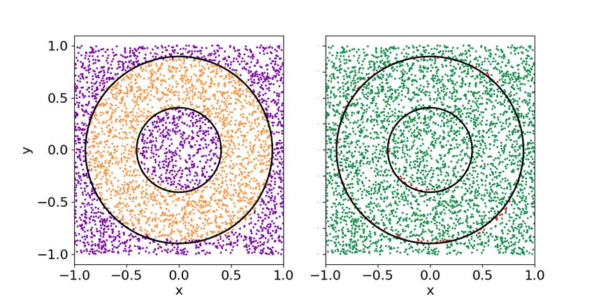
classifiers.                                                          times along the quantum computation.
   A crucial part of a quantum classification algorithm                  We shall illustrate the power of a single- and multi-
is how data is encoded into the circuit. Proposals                    qubit classifiers with data re-uploading with a series
based on kernel methods design an encoding circuit                    of examples. First, we classify points in a plane that
which implements a feature map from the data space                    is divided into two areas. Then, we extend the num-
to the qubits Hilbert space. The construction of this                 ber of regions on a plane to be classified. Next, we
quantum feature map may vary depending on the al-                     consider the classification of multi-dimensional pat-
gorithm, but common strategies make use of the quan-                  terns and, finally, we benchmark this quantum clas-
tum Fourier transform or introduce data in multiple                   sifier with non-convex figures. For every example,
qubits using one- and two-qubit gates [9, 10]. Both                   we train a parametrized quantum circuit that car-
the properties of the tensor product and the entangle-                ries out the task and we analyze its performance in
ment generated in those encoding circuits capture the                 terms of the circuit architecture, i.e., for single- and
non-linearities of the data. In contrast, we argue that               multi-qubit classifiers with and without entanglement
there is no need to use highly sophisticated encoding                 between qubits.
circuits nor a significant number of qubits to intro-                    This paper is structured as follows. First, in Sec-
duce these non-linearities. Single-qubit rotations ap-                tion 2, we present the basic structure of a single-qubit
plied multiple times along the circuit generate highly                quantum classifier. Data and processing parameters
non-trivial functions of the data values. The main dif-               are uploaded and re-uploaded using one-qubit gen-
ference between our approach and the ones described                   eral rotations. For each data point, the final state
above is that the circuit is not divided between the                  of the circuit is compared with the target state as-
encoding and processing parts, but implements both                    signed to its class, and the free parameters of the cir-
multiple times along the algorithm.                                   cuit are updated accordingly using a classical mini-
   Data re-uploading is considered as a manner of solv-               mization algorithm. Next, in Section 3, we motivate
ing the limitations established by the no-cloning the-                the data re-uploading approach by using the Univer-
orem. Quantum computers cannot copy data, but                         sal Approximation Theorem of artificial neural net-
classical devices can. For instance, a neural network                 works. In Section 4, we introduce the extension of
takes the same input many times when processing the                   this classifier to multiple qubits. Then, in Section 5,
data in the hidden layer neurons. An analogous quan-                  we detail the minimization methods used to train the
tum neural network can only use quantum data once.                    quantum classifiers. Finally, in Section 6, we bench-
Therefore, it makes sense to re-upload classical data                 mark single- and multi-qubit quantum classifiers de-
along a quantum computation to bypass this limita-                    fined previously with problems of different dimensions
tion on the quantum circuit. By following this line                   and complexity and compare their performance re-
of thought, we present an equivalence between data                    spect to classical classification techniques. The con-
re-uploading and the Universal Approximation The-                     clusions of this proposal for a quantum classifier are
orem applied to artificial neural networks [12]. Just                 exposed in Section 7.
as a network composed of a single hidden layer with
enough neurons can reproduce any continuous func-
tion, a single-qubit classifier can, in principle, achieve            2 Structure of a single-qubit quantum
the same by re-uploading the data enough times.                       classifier
   The single-qubit classifier illustrates the computa-
tional power that a single qubit can handle. This pro-                The global structure of any quantum circuit can be
posal is to be added to other few-qubit benchmarks                    divided into three elements: uploading of informa-
in machine learning [13]. The input redundancy has                    tion onto a quantum state, processing of the quan-
also been proposed to construct complex encoding in                   tum state, and measurement of the final state. It is
parametrized quantum circuits and in the construc-                    far from obvious how to implement each of these ele-
tion of quantum feature maps [10, 14]. These and                      ments optimally to perform a specific operation. We
other proposals mentioned in the previous paragraphs                  shall now address them one at a time for the task of
are focused on representing classically intractable or                classification.
very complex kernel functions with few qubits. On
the contrary, the focus of this work is to distill the                2.1 Re-uploading classical information
minimal amount of quantum resources, i.e., the num-
ber of qubits and gates, needed for a given classifica-               To load classical information onto a quantum circuit is
tion task quantified in terms of the number of qubits                 a highly non-trivial task [4]. A critical example is the
and unitary operations. The main result of this work                  processing of big data. While there is no in-principle
is, indeed, to show that there is a trade-off between                 obstruction to upload large amounts of data onto a
the number of qubits needed to perform classification                 state, it is not obvious how to do it.
and multiple data re-uploading. That is, we may use                      The problem we address here is not related to a
fewer qubits at the price of re-entering data several                 large amount of data. It is thus possible to consider a

Accepted in   Quantum 2020-01-27, click title to verify. Published under CC-BY 4.0.                                         2
quantum circuit where all data are loaded in the co-
efficients of the initial wave function [8, 9, 13–15]. In
the simplest of cases, data are uploaded as rotations of
qubits in the computational basis. A quantum circuit
would then follow that should perform some classifi-
cation.
   This strategy would be insufficient to create a uni-
versal quantum classifier with a single qubit. A first
limitation is that a single qubit only has two degrees
of freedom, thus only allowing to represent data in                     (a) Neural network            (b) Quantum classifier
a two-dimensional space. No quantum classifier in
higher dimensions can be created if this architecture                 Figure 1: Simplified working schemes of a neural network
is to be used. A second limitation is that, once data                 and a single-qubit quantum classifier with data re-uploading.
is uploaded, the only quantum circuit available is a                  In the neural network, every neuron receives input from all
rotation in the Bloch sphere. It is easy to prove that                neurons of the previous layer. In contrast with that, the
a single rotation cannot capture any non-trivial sepa-                single-qubit classifier receives information from the previous
ration of patterns in the original data.                              processing unit and the input (introduced classically). It pro-
   We need to turn to a different strategy, which turns               cesses everything all together and the final output of the
out to be inspired by neural networks. In the case of                 computation is a quantum state encoding several repetitions
                                                                      of input uploads and processing parameters.
feed-forward neural networks, data are entered in a
network in such a way that they are processed by sub-
sequent layers of neurons. The key idea is to observe                 quantum classifier will depend on the number of re-
that the original data are processed several times, one               uploads of classical data. This fact will be explored
for each neuron in the first hidden layer. Strictly                   in the results section.
speaking, data are re-uploaded onto the neural net-
work. If neural networks were affected by some sort
of no-cloning theorem, they could not work as they                    2.2 Processing along re-uploading
do. Coming back to the quantum circuit, we need to                    The single-qubit classifier belongs to the category of
design a new architecture where data can be intro-                    parametrized quantum circuits. The performance of
duced several times into the circuit.                                 the circuit is quantified by a figure of merit, some
   The central idea to build a universal quantum clas-                specific χ2 to be minimized and defined later. We
sifier with a single qubit is thus to re-upload classical             need, though, to specify the processing gates present
data along with the computation. Following the com-                   in the circuit in terms of a classical set of parameters.
parison with an artificial neural network with a single                  Given the simple structure of a single-qubit circuit
hidden layer, we can represent this re-upload diagram-                presented in Figure 2, the data is introduced in a sim-
matically, as it is shown in Figure 1. Data points in a               ple rotation of the qubit, which is easy to character-
neural network are introduced in each processing unit,                ize. We just need to use arbitrary single-qubit rota-
represented with squares, which are the neurons of the                                                                  ~ with
                                                                      tions U (φ1 , φ2 , φ3 ) ∈ SU(2). We will write U (φ)
hidden layer. After the neurons process these data, a                 ~ = (φ1 , φ2 , φ3 ). Then, the structure of the universal
                                                                      φ
final neuron is necessary to construct the output to be               quantum classifier made with a single qubit is
analyzed. Similarly, in the single-qubit quantum clas-
sifier, data points are introduced in each processing                             ~ ~x) ≡ U (φ
                                                                                U(φ,         ~ N )U (~x) . . . U (φ
                                                                                                                  ~ 1 )U (~x),   (1)
unit, which this time corresponds to a unitary rota-
tion. However, each processing unit is affected by the                which acts as
                                                                                                    ~ ~x)|0i.
                                                                                            |ψi = U(φ,                           (2)
previous ones and re-introduces the input data. The
final output is a quantum state to be analyzed as it                    The final classification of patterns will come from
will be explained in the next subsections.                            the results of measurements on |ψi. We may introduce
   The explicit form of this single-qubit classifier is               the concept of processing layer as the combination
shown in Figure 2. Classical data are re-introduced
                                                                                                     ~ i )U (~x),
                                                                                           L(i) ≡ U (φ                           (3)
several times in a sequence interspaced with process-
ing units. We shall consider the introduction of data
                                                                      so that the classifier corresponds to
as a rotation of the qubit. This means that data from
three-dimensional space, ~x, can be re-uploaded using                                    ~ ~x) = L(N ) . . . L(1),
                                                                                       U(φ,                                      (4)
unitaries that rotate the qubit U (~x). Later processing
units will also be rotations as discussed later on. The               where the depth of the circuit is 2N . The more layers
whole structure needs to be trained in the classifica-                the more representation capabilities the circuit will
tion of patterns.                                                     have, and the more powerful the classifier will be-
   As we shall see, the performance of the single-qubit               come. Again, this follows from the analogy to neural

Accepted in   Quantum 2020-01-27, click title to verify. Published under CC-BY 4.0.                                                3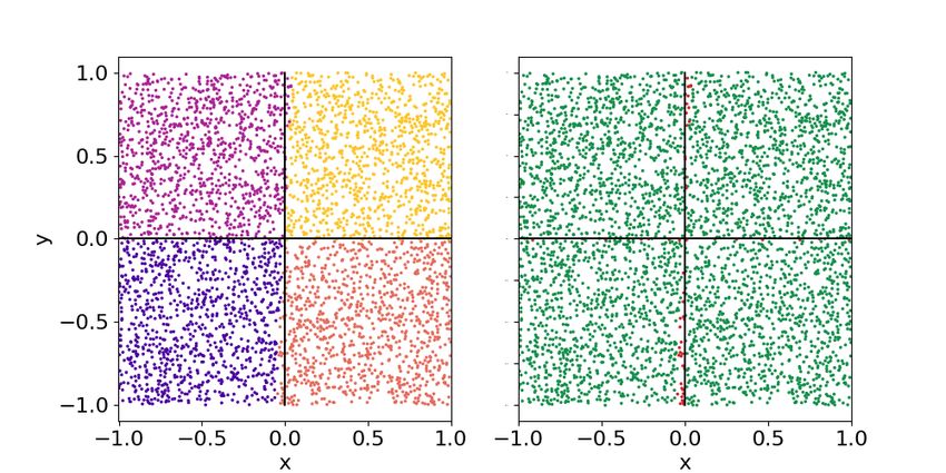
L(1)                         L(N )
                                                                            other encoding techniques, e.g. the ones proposed in
                                                                            Ref. [10], but for the scope of this work, we have
|0i       U (~x)             ~1)
                          U (φ     ···    U (~x)          ~N )
                                                       U (φ                 just tested the linear encoding strategy as a proof of
                                                                            concept of the performance of this quantum classifier.
                               (a) Original scheme                            It is also possible to enlarge the dimensionality of
                                                                            the input space in the following way. Let us extend
                    L(1)                           L(N )
                                                                            the definition of i-th layer to

                                                                                         (k)     (k)                 (1)   (1)

|0i            U φ~ 1 , ~x         ···         U φ~ N , ~x                  L(i) = U θ~i + w   ~ i ◦ ~x(k) · · · U θ~i + w
                                                                                                                         ~ i ◦ ~x(1) ,
                                                                                                                                 (6)
                                                                            where each data point is divided into k vectors of di-
                             (b) Compressed scheme                          mension three. In general, each unitary U could ab-
                                                                            sorb as many variables as freedom in an SU(2) uni-
      Figure 2: Single-qubit classifier with data re-uploading. The         tary. Each set of variables act at a time, and all of
      quantum circuit is divided into layer gates L(i), which con-          them have been shown to the circuit after k iterations.
      stitutes the classifier building blocks. In the upper circuit,        Then, the layer structure follows. The complexity of
      each of these layers is composed of a U (~ x) gate, which up-         the circuit only increases linearly with the size of the
      loads the data, and a parametrized unitary gate U (φ).~ We            input space.
      apply this building block N times and finally compute a cost
      function that is related to the fidelity of the final state of
      the circuit with the corresponding target state of its class.         2.3 Measurement
      This cost function may be minimized by tunning the φ    ~ i pa-
      rameters. Eventually, data and tunable parameters can be              The quantum circuit characterized by a series of pro-
      introduced with a single unitary gate, as illustrated in the          cessing angles {θi } and weights {wi } delivers a final
      bottom circuit.                                                       state |ψi, which needs to be measured. The results
                                                                            of each measurement are used to compute a χ2 that
                                                                            quantifies the error made in the classification. The
      networks, where the size of the intermediate hidden                   minimization of this quantity in terms of the classical
      layer of neurons is critical to represent complex func-               parameters of the circuit can be organized using any
      tions.                                                                preferred supervised machine learning technique.
         There is a way to compactify the quantum circuit                      The critical point in the quantum measurement is
      into a shorter one. This can be done if we incorporate                to find an optimal way to associate outputs from the
      data and processing angles in a single step. Then, a                  observations to target classes. The fundamental guid-
      layer would only need a single rotation to introduce                  ing principle to be used is given by the idea of max-
      data and tunable parameters, i.e. L(i) = U (φ,~ ~x). In               imal orthogonality of outputs [16]. This is easily es-
      addition, each data point can be uploaded with some                   tablished for a dichotomic classification, where one of
      weight wi . These weights will play a similar role as                 two classes A and B have to be assigned to the final
      weights in artificial neural networks, as we will see in              measurement of the single qubit. In such a case it
      the next section. Altogether, each layer gate can be                  is possible to measure the output probabilities P (0)
      taken as                                                            for |0i and P (1) for |1i. A given pattern could be
                      L(i) = U θ~i + w ~ i ◦ ~x ,          (5)              classified into the A class if P (0) > P (1) and into B
                                                                           otherwise. We may refine this criterium by introduc-
      where w ~ i ◦ ~x = wi1 x1 , wi2 x2 , wi3 x3 is the Hadamard           ing a bias. That is, the pattern is classified as A if
      product of two vectors. In case the data points have                  P (0) > λ, and as B otherwise. The λ is chosen to op-
      dimension lesser than three, the rest of ~x components                timize the success of classification on a training set.
      are set to zero. Such an approach reduces the depth of                Results are then checked on an independent validation
      the circuit by half. Further combinations of layers into              set.
      fewer rotations are also possible, but the nonlinearity                  The assignment of classes to the output reading of
      inherent to subsequent rotations would be lost, and                   a single qubit becomes an involved issue when many
      the circuit would not be performing well.                             classes are present. For the sake of simplicity, let us
        Notice that data points are introduced linearly into                mention two examples for the case of classification to
      the rotational gate. Non-linearities will come from                   four distinct classes. One possible strategy consists on
      the structure of these gates. We chose this encoding                  comparing the probability P (0) to four sectors with
      function as we believe it is one of the lesser biased                 three thresholds: 0 ≤ λ1 ≤ λ2 ≤ λ3 ≤ 1. Then, the
      ways to encode data with unknown properties. Due                      value of P (0) will fall into one of them, and classifi-
      to the structure of single-qubit unitary gates, we will               cation is issued. A second, more robust assignment is
      see that this encoding is particularly suited for data                obtained by computing the overlap of the final state
      with rotational symmetry. Still, it can also classify                 to one of the states of a label states-set. This states-
      other kinds of data structures. We can also apply                     set is to be chosen with maximal orthogonality among

      Accepted in   Quantum 2020-01-27, click title to verify. Published under CC-BY 4.0.                                          4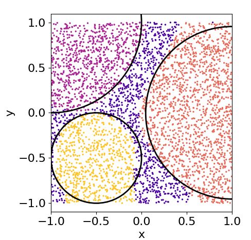
cost function that carries out this task,
                                                                                             M
                                                                                             X
                                                                                   ~ w)
                                                                              χ2f (θ, ~ =                       ~ w,
                                                                                                   1 − |hψ̃s |ψ(θ, ~ x~µ )i|2 ,   (7)
                                                                                             µ=1

                                                                      where |ψ̃s i is the correct label state of the µ data
                                                                      point, which will correspond to one of the classes.

                                                                      2.3.2   A weighted fidelity cost function

Figure 3: Representation in the Bloch sphere of four and six          We shall next define a refined version of the previous
maximally orthogonal points, corresponding to the vertices            fidelity cost function to be minimized. The set of
of a tetrahedron and an octahedron respectively. The single-          maximally orthogonal states in the Bloch sphere, i.e.,
qubit classifier will be trained to distribute the data points in     the label states, are written as |ψc i, where c is the
one of these vertices, each one representing a class.                 class. Each of these label states represents one class
                                                                      for the classifier. Now, we will follow the lead usually
                                                                      taken in neural network classification.
all of them. This second method needs from the max-
                                                                         Let us define the quantity
imally orthogonal points in the Bloch sphere. Figure
3 shows the particular cases that can be applied to                                       ~ w,
                                                                                      Fc (θ,                  ~ w,
                                                                                             ~ ~x) = |hψ̃c |ψ(θ, ~ ~x)i|2 ,       (8)
a classification task of four and six classes. In gen-
eral, a good measurement strategy may need some                       where M is the total number of training points, |ψ̃c i
prior computational effort and refined tomography of                  is the label state of the class c and |ψ(θ,~ w,
                                                                                                                   ~ ~x)i is the
the final state. Since we are proposing a single-qubit                final state of the qubit at the end of the circuit. This
classifier, the tomography protocol will only require                 fidelity is to be compared with the expected fidelity of
three measurements.                                                   a successful classification, Yc (~x). For example, given
   It is possible to interpret the single-qubit classi-               a four-class classification and using the vertices of a
fier in terms of geometry. The classifier opens a 2-                  tetrahedron as label states (as shown in Figure 3),
dimensional Hilbert space, i.e., the Bloch sphere. As                 one expects Ys (~x) = 1, where s is the correct class,
we encode data and classification within the param-                   and Yr (~x) = 1/3 for the other r classes. In general,
eters defining rotations, this Hilbert space is enough                Yc (~x) can be written as a vector with one entry equal
to achieve classification. Any operation L(i) is a ro-                to 1, the one corresponding to the correct class, and
tation on the Bloch sphere surface. With this point                   the others containing the overlap between the correct
of view in mind, we can easily see that we can clas-                  class label state and the other label states.
sify any point using only one unitary operation. We                      With these definitions, we can construct a cost
can transport any point to any other point on the                     function which turns out to be inspired by conven-
Bloch sphere by nothing else than choosing the an-                    tional cost functions in artificial neural networks. By
gles of rotation properly. However, this does not                     weighting the fidelities of the final state of the circuit
work for several data, as the optimal rotation for some               with all label states, we define the weighted fidelity
data points could be very inconvenient for some other                 cost function as
points. However, if more layers are applied, each one
                                                                                                C
                                                                                            M
                                                                                                                                        !
will perform a different rotation, and many different                                    1 X X                                 2
                                                                      χ2wf (~  ~ w)
                                                                            α, θ, ~    =                  ~ w,
                                                                                                   αc Fc (θ, ~ ~xµ ) − Yc (~xµ )            ,
rotations together have the capability of enabling a                                     2 µ=1 c=1
feature map. Data embedded in this feature space
can be easily separated into classes employing the re-                                                                        (9)
gions on the Bloch sphere.                                            where M is the total number of training points, C
                                                                      is the total number of classes, ~xµ are the training
                                                                      points and α ~ = (α1 , · · · , αC ) are introduced as class
2.3.1   A fidelity cost function
                                                                      weights to be optimized together with θ~ and w       ~ pa-
We propose a very simple cost function motivated by                   rameters. This weighted fidelity has more parameters
the geometrical interpretation introduced above. We                   than the fidelity cost function. These parameters are
want to force the quantum states |ψ(θ,~ w,
                                        ~ ~x)i to be as               the weights for the fidelities.
near as possible to one particular state on the Bloch                    The main difference between the weighted fidelity
sphere. The angular distance between the label state                  cost function of Eq. (9) and the fidelity cost function
and the data state can be measured with the relative                  of Eq. (7) is how many overlaps do we need to com-
fidelity between the two states [17]. Thus, our aim                   pute. The χ2wf requires as many fidelities as classes
is to maximize the average fidelity between the states                every time we run the optimization subroutine, while
at the end of the quantum circuit and the label states                the χ2f needs just one. This is not such a big differ-
corresponding to their class. We define the following                 ence for a few classes and only one qubit. It is possible

Accepted in   Quantum 2020-01-27, click title to verify. Published under CC-BY 4.0.                                                5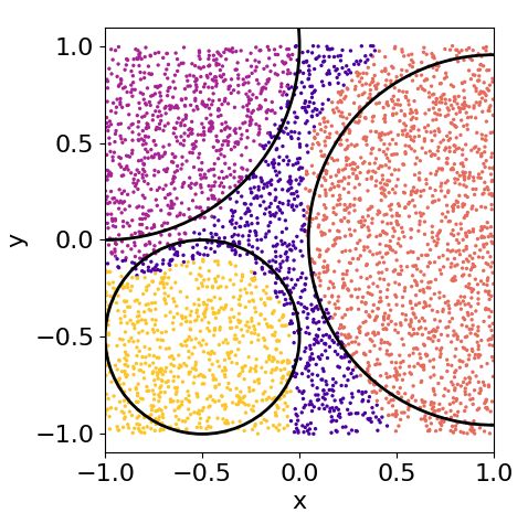
to measure any state with a full tomography process                   that it is possible to reconstruct any continuous func-
which, for one qubit, is achievable. However, for many                tion with a single layer neural network of N neurons.
different classes, we expect that one measurement will                The proof of this theorem for the sigmoidal activation
be more efficient than many.                                          function can be found in Ref. [18]. This theorem was
   Besides the weighted fidelity cost function being                  generalized for any nonconstant, bounded and contin-
costlier than the fidelity cost function, there is another            uous activation function in Ref. [12]. Moreover, Ref.
qualitative difference between both. The fidelity cost                [12] presents the following corollary of this theorem:
function forces the parameters to reach the maximum                   ϕ could be a nonconstant finite linear combination of
in fidelities. Loosely speaking, this fidelity moves the              periodic functions, in particular, ϕ could be a non-
qubit state to where it should be. The weighted fi-                   constant trigonometric polynomial.
delity forces the parameters to be close to a specified
configuration of fidelities. It moves the qubit state to
where it should be and moves it away from where it                    3.2 Universal Quantum Circuit Approximation
should not. Therefore, we expect that the weighted fi-                The single-qubit classifier is divided into several layers
delity will work better than the fidelity cost function.              which are general SU(2) rotational matrices. There
Moreover, this extra cost in terms of the number of                   exist many possible decompositions of an SU(2) rota-
parameters of the weighted fidelity cost function will                tional matrix. In particular, we use
only affect the classical minimization part of the al-
gorithm. In a sense, we are increasing the classical                         ~ = U (φ1 , φ2 , φ3 ) = eiφ2 σz eiφ1 σy eiφ3 σz ,
                                                                          U (φ)                                                         (12)
processing part to reduce the quantum resources re-
quired for the algorithm, i.e. the number of quantum                  where σi are the conventional Pauli matrices. Using
operations (layers). This fact gain importance in the                 the SU(2) group composition law, we can rewrite the
NISQ computation era.                                                 above parametrization in a single exponential,
                                                                                                         ~ σ
                                                                                                ~ = ei~ω(φ)·~
3 Universality of the single-qubit clas-                                                     U (φ)            ,                         (13)

sifier                                                                with ω
                                                                           ~ (φ)

                                                                              ~ = ω1 (φ),
                                                                                      ~ ω2 (φ),
                                                                                            ~ ω3 (φ)

                                                                                                  ~ and

After analyzing several classification problems, we ob-
tain evidence that the single-qubit classifier intro-                          ~ = d N sin ((φ2 − φ3 )/2) sin (φ1 /2) ,
                                                                           ω1 (φ)                                                       (14)
duced above can approximate any classification func-                           ~ = d N cos ((φ2 − φ3 )/2) sin (φ1 /2) ,
                                                                           ω2 (φ)                                                       (15)
tion up to arbitrary precision. In this section, we pro-
                                                                               ~ = d N sin ((φ2 + φ3 )/2) cos (φ1 /2) ,
                                                                           ω3 (φ)                                                       (16)
vide the motivation for this statement based on the
Universal Approximation Theorem (UAT) of artificial                                         √            −1
neural networks [12].                                                 where N        =        1 − cos2 d      and cos d =
                                                                      cos ((φ2 + φ3 )/2) cos (φ1 /2).
3.1 Universal Approximation Theorem                                      The single-qubit classifier codifies the data points
                                                                      into φ~ parameters of the U unitary gate. In particu-
Theorem– Let Im = [0, 1]m be the m-dimensional unit                   lar, we can re-upload data together with the tunable
cube and C(Im ) the space of continuous functions in                  parameters as defined in Eq. (5), i.e.
Im . Let the function ϕ : R → R be a nonconstant,
bounded and continuous function and f : Im → R                             ~ x) = (φ1 (~x), φ2 (~x), φ3 (~x)) = θ~ + w
                                                                           φ(~                                       ~ ◦ ~x.            (17)
a function. Then, for every  > 0, there exists an
integer N and a function h : Im → R, defined as                       Thus,
                          N
                          X                                                                                         N
                                                                                                                                 ~
                                      ~ i · ~x + bi ) ,
                                                                                                                    Y
                h(~x) =         αi ϕ (w                     (10)        U(~x) = UN (~x)UN −1 (~x) · · · U1 (~x) =         ei~ω(φi (~x))·~σ ,
                          i=1                                                                                       i=1
                                      m
                                                                                                                    (18)
with αi , bi ∈ R and w
                     ~ i ∈ R , such that h is an ap-                  Next, we apply the Baker-Campbell-Hausdorff (BCH)
proximate realization of f with precision , i.e.,                    formula [19] to the above equation,
                       |h(~x) − f (~x)| <                  (11)                         "   N
                                                                                                                             #
                                                                                             X
                                                                           U(~x) = exp i           ω  ~ i (~x)) · ~σ + Ocorr .
                                                                                                   ~ (φ                                 (19)
for all ~x ∈ Im .                                                                            i=1
  In artificial neural networks, ϕ is the activation
function, w ~ i are the weights for each neuron, bi are the           Notice that the remaining BCH terms Ocorr are
biases and αi are the neuron weights that construct                   also proportional to Pauli matrices due to [σi , σj ] =
the output function. Thus, this theorem establishes                   2iijk σk .

Accepted in   Quantum 2020-01-27, click title to verify. Published under CC-BY 4.0.                                                            6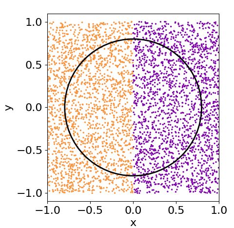
Each ω~ terms are trigonometric functions, uncon-                             To circumvent this inconvenience, more hidden layers
stant, bounded and continuous. Then                                             are introduced, leading eventually to the concept of
                                                                                deep neural networks.
     N                    N
   X                    X                                                         By using the single-qubit classifier formalism that
         ω  ~ i (~x)) =
         ~ (φ                       ~ i (~x)), ω2 (φ
                                ω1 (φ               ~ i (~x)), ω3 (φ
                                                                   ~ i (~x))
                                                                                we have introduced in the previous sections, we pro-
    i=1                  i=1                                                    pose its generalization to more qubits. The introduc-
    X N                                                                       tion of multiple qubits to this quantum classifier may
 =         ω1 (θ~i + w~ i ◦ ~x), ω2 (θ~i + w ~ i ◦ ~x), ω3 (θ~i + w~ i ◦ ~x) improve its performance as more hidden layers im-
     i=1
                                                                                prove the classification task of an artificial neural net-
                                 = (f1 (~x), f2 (~x), f3 (~x)) . (20)           work. With the introduction of entanglement between
                                                                                these qubits, we reduce the number of layers of our
   We still have to deal with the remaining terms
                                                                                classifier as well as propose a quantum classification
Ocorr of the BCH expansion. Instead of applying
                                                                                method that can achieve quantum advantage.
such expansion, we can use again the SU(2) group
                                                                                   Figure 1 shows the analogy between a neural net-
composition law to obtain the analytical formula of
               ~                 ~ x) will be an inextricably                   work   with a single hidden layer and a single-qubit
U(~x) = eiξ(~x)·~σ , where ξ(~                                                  classifier. The generalization of this analogy is not
trigonometric function of ~x. The Ocorr terms are pro-                          so obvious. A multi-qubit classifier without entan-
portional to ~σ matrices, so Ocorr = %              ~(~x) · ~σ for some         glement could have some similarities with a convolu-
function %  ~(~x). Then,                                                        tional neural network, where each qubit could repre-
                           ~              ~                                     sent a neural network by itself. However, it is not clear
              U(~x) = eiξ(~x)·~σ = eif (~x)·~σ+i~%(~x)·~σ .           (21)
                                                                                if the introduction of entanglement between qubits
                                                                                can be understood as a deep neural network archi-
Thus, Ocorr terms can be absorbed in f~(~x).
                                                                                tecture. The discussion around this analogy as well
   For each data point ~x, we obtain a final state that
                           ~ x) functions. With all train-                      as an extended study of the performance of a multi-
will contain these ξ(~
                                                                                qubit classifier is beyond the scope of this work. In
ing points, we construct a cost function that can in-
                                                                                the next subsections, we present a general proposal
clude new parameters αc for each class if we use the
                                                                                for a multi-qubit classifier which we compare with the
weighted fidelity cost function of Eq. (9). The func-
                                                        ~                       single-qubit one in Section 6.
tion obtained from the combination of ξ(x)                     and αc is
expected to be complex enough to probably represent
almost any continuous function. However, more pa-                               4.1 Measurement strategy and cost function
rameters are necessary to map this argument with the                            for a multi-qubit classifier
UAT expression.
   If we compare the parameters of the UAT with the                             With a single-qubit classifier, the measurement strat-
single-qubit circuit parameters, the w            ~ i will correspond           egy consisting on comparing the final state of the
                              ~
with the weights, the θi with the biases bi , the number                        circuit with a pre-defined target state was achiev-
of layers N of the quantum classifier will correspond                           able. Experimentally, one needs to perform a quan-
with the number of neurons in the hidden layer and                              tum state tomography protocol of only three mea-
ω
~ functions with the activation functions ϕ.                                    surements. However, if more qubits are to be con-
   We have explained why it is necessary to re-upload                           sidered, tomography protocols become exponentially
the data at each layer and why a single qubit could                             expensive in terms of number of measurements.
be a universal classifier. As has been stated before,                              We propose two measurement strategies for a multi-
an artificial neural network introduces the data points                         qubit classifier. The first one is the natural general-
in each hidden neuron, weights them and adds some                               ization of the single-qubit strategy, although it will
bias. Here we cannot just copy each data point be-                              become unrealizable for a large number of qubits. We
cause the non-cloning theorem, so we have to re-                                compare the final state of the circuit with one of the
upload it at each layer.                                                        states of the computational basis, one for each class.
                                                                                The second strategy consist on focusing in one qubit
                                                                                and depending on its state associate one or other class.
4 From single- to multi-qubit quantum This is similar to previous proposals of binary multi-
classifier                                                                      qubit classifiers [7], although we add the possibility of
                                                                                multiclass classification by introducing several thresh-
The single-qubit classifier cannot carry any quantum                            olds (see Section 2).
advantage respect classical classification techniques                              Another part that should be adapted is the defini-
such as artificial neural networks. In the previous                             tion of the cost function. In particular, we use differ-
sections, we have defined a quantum mechanical ver-                             ent functions for each strategy explained above.
sion of a neural network with a single hidden layer. In                            For the first strategy, we use the fidelity cost func-
general, a huge amount of hidden neurons is necessary                           tion of Eq. (7). Its generalization to more qubits is
to approximate a target function with a single layer.                           straightforward. However, the orthogonal states used

Accepted in   Quantum 2020-01-27, click title to verify. Published under CC-BY 4.0.                                                     7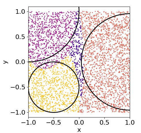
|0i        L1 (1)      L1 (2)       L1 (3)   ···    L1 (N )           |0i       L1 (1)        L1 (2)     L1 (3)    ···    L1 (N )

|0i        L2 (1)      L2 (2)       L2 (3)   ···    L2 (N )           |0i       L2 (1)        L2 (2)     L2 (3)    ···    L2 (N )

                (a) Ansatz with no entanglement
                                                                      |0i       L3 (1)        L3 (2)     L3 (3)    ···    L3 (N )

                                                                      |0i       L4 (1)        L4 (2)     L4 (3)    ···    L4 (N )
|0i         L1 (1)     •   L1 (2)     • ··· •       L1 (N )

|0i         L2 (1)     •   L2 (2)     • ··· •       L2 (N )                           (a) Ansatz with no entanglement

                  (b) Ansatz with entanglement
                                                                      |0i      L1 (1)     •     L1 (2)        • ··· •     L1 (N )

Figure 4: Two-qubit quantum classifier circuit without en-            |0i      L2 (1)     •     L2 (2)    •       ··· •   L2 (N )
tanglement (top circuit) and with entanglement (bottom
circuit). Here, each layer includes a rotation with data re-          |0i      L3 (1)     •     L3 (2)    •       ··· •   L3 (N )
uploading in both qubits plus a CZ gate if there is entangle-
ment. The exception is the last layer, which does not have            |0i      L4 (1)     •     L4 (2)        • ··· •     L4 (N )
any CZ gate associated to it. For a fixed number of layers,
the number of parameters to be optimized doubles the one
needed for a single-qubit classifier.                                                   (b) Ansatz with entanglement

                                                                      Figure 5: Four-qubit quantum classifier circuits. Without
for a multi-qubit classifier are taken as the computa-                entanglement (top circuit), each layer is composed by four
tional basis states. A more sophisticated set of states               parallel rotations. With entanglement (bottom circuit) each
could be considered to improve the performance of                     layer includes a parallel rotation and two parallel CZ gates.
this method.                                                          The order of CZ gates alternates in each layer between (1)-
   For the second strategy, we use the weighted fidelity              (2) and (3)-(4) qubits and (2)-(3) and (1)-(4) qubits. The
cost function. As stated above, we just focus on one                  exception is in the last layer, which does not contain any CZ
qubit, thus                                                           gate. For a fixed number of layers, the number of parameters
                                                                      to be optimized quadruples the ones needed for a single-qubit
                    ~ w,
              Fc,q (θ,                   ~ w,
                       ~ ~x) = hψ̃c |ρq (θ, ~ ~x)|ψ̃c i,      (22)    classifier.

where ρq is the reduced density matrix of the qubit to
be measured. Then, the weighted fidelity cost func-                   correct ansatz for the entangling structure of the cir-
tion can be adapted as                                                cuit.
                                                                         Figures 4 and 5 show the explicit circuits used in
  χ2wf (~  ~ w)
        α, θ, ~ =                                                     this work. For a two-qubit classifier without entangle-
         M   C   Q                                   2
                                                              !       ment, and similarly for a four-qubit classifier, we iden-
      1 XX X                  ~ w,                                   tify each layer as parallel rotations on all qubits. We
                    αc,q Fc,q (θ, ~ ~xµ ) − Yc (~xµ )             ,
      2 µ=1 c=1 q=1                                                   introduce the entanglement using CZ gates between
                                                              (23)    rotations that are absorbed in the definition of layer.
                                                                      For two-qubit classifier with entanglement, we apply a
where we average over all Q qubits that form the clas-                CZ gate after each rotation with exception of the last
sifier. Eventually, we can just measure one of these                  layer. For a four-qubit classifier, two CZ gates are ap-
qubits, reducing the number of parameters to be op-                   plied after each rotation alternatively between (1)-(2)
timized.                                                              and (3)-(4) qubits and (2)-(3) and (1)-(4) qubits.
                                                                         The number of parameters needed to perform the
4.2 Quantum circuits examples                                         optimization doubles the ones needed for a single-
                                                                      qubit classifier for the two-qubit classifier and quadru-
The definition of a multi-qubit quantum classifier cir-               ples for the four-qubit classifier. For N layers, the cir-
cuit could be as free as is the definition of a multi-                cuit depth is N for the non-entangling classifiers and
layer neural network. In artificial neural networks,                  2N for the entangling classifiers.
it is far from obvious what should be the number of
hidden layers and neurons per layer to perform some
task. Besides, it is, in general, problem-dependent.                  5 Minimization methods
For a multi-qubit quantum classifier, there is extra
degree of freedom in the circuit-design: how to in-                   The practical training of a parametrized single-qubit
troduce the entanglement. This is precisely an open                   or multi-qubit quantum classifier needs minimization
problem in parametrized quantum circuits: to find a                   in the parameter space describing the circuit. This

Accepted in   Quantum 2020-01-27, click title to verify. Published under CC-BY 4.0.                                                 8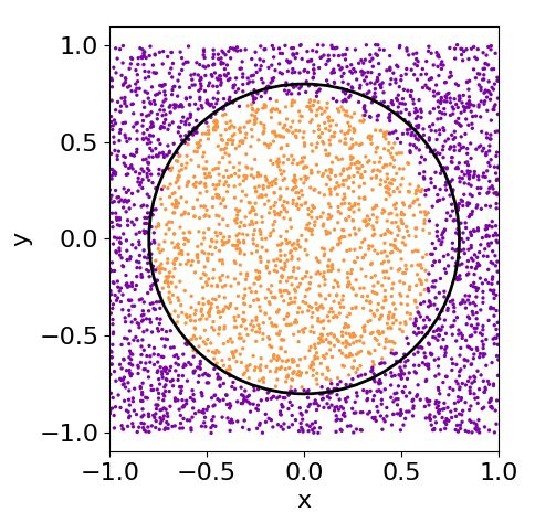
is often referred as a hybrid algorithm, where classi-                networks have got huge products of non linear func-
cal and quantum logic coexist and benefit from one                    tions. The odds of having local minima are then large.
another. To be precise, the set of {θi } angles and                   In the quantum circuits side, there are nothing but
{wi } weights, together with αq,l parameters if appli-                trigonometric functions. In both cases, if there are a
cable, forms a space to be explored in search of a min-               lot of training points it is more likely to find some of
imum χ2 . In parameter landscapes as big as the ones                  them capable of getting us out of local minima. If this
treated here, or in regular neural network classifica-                is the case, SGD is more useful for being faster. On
tion, the appearance of local minima is ultimately un-                the contrary, when the training set is small, we have
avoidable. The composition of rotation gates renders                  to pick an algorithm less sensitive to local minima,
a large product of independent trigonometric func-                    such as the L-BFGS-B.
tions. It is thus clear to see that our problem will
be overly populated with minima. The classical min-
imizer can easily get trapped in a not optimal one.                   6 Benchmark of a single- and multi-
   Our problem is reduced to minimizing a function                    qubit classifier
of many parameters. For a single-qubit classifier, the
number of parameters is (3 + d)N where d is the di-                   We can now tackle some classification problems. We
mension of the problem, i.e. the dimension of ~x, and                 will prove that a single-qubit classifier can perform
N is the number of layers. Three of these parameters                  a multi-class classification for multi-dimensional data
are the rotational angles and the other d correspond                  and that a multi-qubit classifier, in general, improves
with the w ~ i weight. If using the weighted fidelity cost            these results.
function, we should add C extra parameters, one for                      We construct several classifiers with different num-
each class.                                                           ber of layers. We then train the circuits with a train-
   In principle, one does not know how is the parame-                 ing set of random data points to obtain the values of
ter landscape of the cost function to be minimized. If                the free parameters {θi } and {wi } for each layer and
the cost function were, for example, a convex function,               {αi } when applicable. We use the cost functions de-
a downhill strategy would be likely to work properly.                 fined in Eq. (9) and Eq. (7). Then, we test the perfor-
The pure downhill strategy is known as gradient de-                   mance of each classifier with a test set independently
scent. In machine learning, the method commonly                       generated and one order of magnitud greater than the
used is a Stochastic Gradient Descent (SGD) [20].                     training set. For the sake of reproducibility, we have
   There is another special method of minimization                    fixed the same seed to generate all data points. For
known as L-BFGS-B [21]. This method has been used                     this reason, the test and training set points are the
in classical machine learning with very good results                  same for all problems. For more details, we provide
[22].                                                                 the explicit code used in this work [24].
   The results we present from now on are starred by                     We run a single-, two- and four-qubit classifiers,
the L-BFGS-B algorithm, as we found it is accurate                    with and without entanglement, using the two cost
and relatively fast. We used open source software [23]                functions described above. We benchmark several
as the core of the minimization with own made func-                   classifiers formed by L = 1, 2, 3, 4, 5, 6, 8 and 10 layers.
tions to minimize. The minimizer is taken as a black                     In the following subsections, we describe the partic-
box whose parameters are set by default. As this is                   ular problems addressed with these single- and multi-
the first attempt of constructing a single- or multi-                 qubit classifiers with data re-uploading. We choose
qubit classifier, further improvements can be done on                 four problem types: a simple binary classification,
the hyperparameters of minimization.                                  a classification of a figure with multiple patterns, a
                                                                      multi-dimensional classification and a non-convex fig-
   Nevertheless we have also tested a SGD algorithm
                                                                      ure.
for the fidelity cost function. This whole algorithm
                                                                         The code used to define and benchmark the single-
has been developed by us following the steps from [17].
                                                                      and multi-qubit quantum classifier is open and can be
The details can be read in Appendix A. In general, we
                                                                      found in Ref. [24].
found that L-BFGS-B algorithm is better than SGD.
This is something already observed in classical neu-
ral networks. When the training set is small, it is                   6.1 Simple example: classification of a circle
often more convenient to use a L-BFGS-B strategy
                                                                      Let us start with a simple example. We create a ran-
than a SGD. We were forced to use small training
                                                                      dom set of data on a plane with coordinates ~x =
sets due to computational capabilities for our simula-
                                                                      (x1 , x2 ) with xi ∈ [−1, 1]. Our goal is to classify these
tions. Numerical evidences on this arise when solving
                                                                      points according to x21 +x22 < r2 , i.e. if they are inside
the problems we face for these single- and multi-qubit
                                                                      or outside of a circle of radius r. The value of the ra-
classifiers with classical standard machine learning li-
                                                                      dius is chosen in such a way that the q areas inside and
braries [22]. This can be understood with a simple
argument. Neural networks or our quantum classifier                   outside it are equal, that is, r = π2 , so the proba-
are supposed to have plenty of local minima. Neural                   bility of success if we label each data point randomly

Accepted in   Quantum 2020-01-27, click title to verify. Published under CC-BY 4.0.                                             9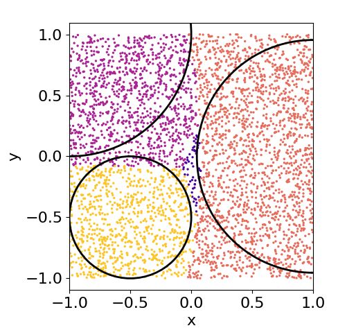
χ2f χ2wf
Qubits 1 2 1 2 4
Layers No Ent. Ent. No Ent. Ent. No Ent. Ent.
1 0.50 0.75 – 0.50 0.76 – 0.76 –
2 0.85 0.80 0.73 0.94 0.96 0.96 0.96 0.96
3 0.85 0.81 0.93 0.94 0.97 0.95 0.97 0.96
4 0.90 0.87 0.87 0.94 0.97 0.96 0.97 0.96
5 0.89 0.90 0.93 0.96 0.96 0.96 0.96 0.96
6 0.92 0.92 0.90 0.95 0.96 0.96 0.96 0.96
8 0.93 0.93 0.96 0.97 0.95 0.97 0.95 0.96
10 0.95 0.94 0.96 0.96 0.96 0.96 0.96 0.97
Table 1: Results of the single- and multi-qubit classifiers with data re-uploading for the circle problem. Numbers indicate the
success rate, i.e. number of data points classified correctly over total number of points. Words “Ent.” and “No Ent.” refer
to considering entanglement between qubits or not, respectively. We have used the L-BFGS-B minimization method with the
weighted fidelity and fidelity cost functions. For this problem, both cost functions lead to high success rates. The multi-qubit
classifier increases this success rate but the introduction of entanglement does not affect it significantly.
is 50%. We create a train dataset with 200 random
entries. We then validate the single-qubit classifier
against a test dataset with 4000 random points.
The results of this classification are written in Ta-
ble 1. With the weighted fidelity cost function, the
single-qubit classifier achieves more than 90% of suc-
cess with only two layers, that is, 12 parameters. The
results are worse with the fidelity cost function. For
(a) 1 layer (b) 2 layers
a two-qubit and a four-qubit classifier, two layers are
required to achieve 96% of success rate, that is, 22 pa-
rameters for the two-qubit and 42 for the four-qubit.
The introduction of entanglement does not change the
result in any case. The results show a saturation of
the success rate. Considering more layers or more
qubits does not change this success rate.
The characterization of a closed curved is a hard
problem for an artificial neural network that works
in a linear regime, although enough neurons, i.e. lin- (c) 4 layers (d) 8 layers
ear terms, can achieve a good approximation to any
function. On the contrary, the layers of a single-qubit Figure 6: Results of the circle classification obtained with a
classifier are rotational gates, which have an intrinsic single-qubit classifier with different number of layers using the
non-linear behavior. In a sense, a circle becomes an L-BFGS-B minimizer and the weighted fidelity cost function.
easy function to classify as a linear function is for an With one layer, the best that the classifier can do is to divide
artificial neural network. The circle classification is, the plane in half. With two layers, it catches the circular
shape which is readjusted as we consider more layers.
in a sense, trivial for a quantum classifier. We need
to run these classifiers with more complex figures or
problems to test their performance.
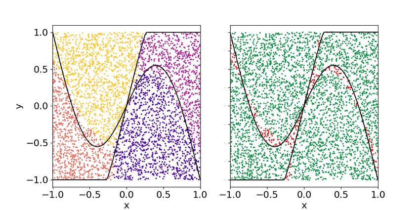
6.2 Classification of multiple patterns
It is interesting to compare classifiers with different We want to show now that the single-qubit classifier
number of layers. Figure 6 shows the result of the can solve multi-class problems. We divide a 2D plane
classification for a single-qubit classifier of 1, 2, 4 and into several regions and assign a label to each one.
8 layers. As with only one layer the best classification We propose the following division: three regions cor-
that can be achieved consist on dividing the plane in responding to three circular sectors and the interme-
half, with two layers the classifier catches the circular diate space between them. We call this problem the
shape. As we consider more layers, the single-qubit 3-circles problem. This is a hardly non-linear prob-
classifier readjust the circle to match the correct ra- lem and, consequently, difficult to solve for a classical
dius. neural network in terms of computational power.
Accepted in Quantum 2020-01-27, click title to verify. Published under CC-BY 4.0. 10χ2f χ2wf
Qubits 1 2 1 2 4
Layers No Ent. Ent. No Ent. Ent. No Ent. Ent.
1 0.73 0.56 – 0.75 0.81 – 0.88 –
2 0.79 0.77 0.78 0.76 0.90 0.83 0.90 0.89
3 0.79 0.76 0.75 0.78 0.88 0.89 0.90 0.89
4 0.84 0.80 0.80 0.86 0.84 0.91 0.90 0.90
5 0.87 0.84 0.81 0.88 0.87 0.89 0.88 0.92
6 0.90 0.88 0.86 0.85 0.88 0.89 0.89 0.90
8 0.89 0.85 0.89 0.89 0.91 0.90 0.88 0.91
10 0.91 0.86 0.90 0.92 0.90 0.91 0.87 0.91
Table 2: Results of the single- and multi-qubit classifiers with data re-uploading for the 3-circles problem. Numbers indicate
the success rate, i.e. number of data points classified correctly over total number of points. Words “Ent.” and “No Ent.”
refer to considering entanglement between qubits or not, respectively. We have used the L-BFGS-B minimization method with
the weighted fidelity and fidelity cost functions. Weighted fidelity cost function presents better results than the fidelity cost
function. The multi-qubit classifier reaches 0.90 success rate with a lower number of layers than the single-qubit classifier.
The introduction of entanglement slightly increases the success rate respect the non-entangled circuit.
Table 2 shows the results for this four-class prob-
lem. For a single-qubit classifier, a maximum of 92%
of success is achieved with 10 layers, i.e. 54 parame-
ters. From these results, it seems that this problem
also saturates around 91% of success. However, the
introduction of more qubits and entanglement makes
possible this result possible with less parameters. For
two qubits with entanglement, 4 layers are necessary
to achieve the same success as with a single-qubit, i.e.
34 parameters. For four qubits without entanglement (a) 1 layer (b) 3 layers
4 layers are also required. Notice also that, although
the number of parameters increases significantly with
the number of qubits, some of the effective operations
are performed in parallel.
There is an effect that arises from this more com-
plex classification problem: local minima. Notice that
the success rate can decrease when we add more layers
into our quantum classifier.
As with the previous problem, it is interesting to
compare the performance in terms of sucess rate of
(c) 4 layers (d) 10 layers
classifiers with different number of layers. Figure 7
shows the results for a two-qubit classifier with no en-
Figure 7: Results for the 3-circles problem using a single-
tanglement for 1, 3, 4 and 10 layers. Even with only
qubit classifier trained with the L-BFGS-B minimizer and the
one layer, the classifier identifies the four regions, be-
weighted fidelity cost function. With one layer, the classifier
ing the more complicated to describe the central one. intuits the four regions although the central one is difficult
As we consider more layers, the classifier performs to tackle. With more layers, this region is clearer for the
better and adjust these four regions. classifier and it tries to adjust the circular regions.
6.3 Classification in multiple dimensions
kind of data if we apply enough gates.
As explained in Section 2, there is no restriction in Following this idea we will now move to a more
uploading multidimensional data. We can upload up complicated classification using data with 4 coordi-
to three values per rotation since this is the degrees of nates. We use as a problem the four-dimensional
freedom of a SU(2) matrix. If the dimension of data is sphere, i.e. classifying data points according to
larger than that, we can just split the data vector into x21 + x22 + x23 + x24 < 2/π. Similarly with the previous
subsets and upload each one at a time, as described problems, xi ∈ [−1, 1] and the radius has been chosen
explicitly in Eq. (6). Therefore, there is no reason to such that the volume of the hypersphere is half of the
limit the dimension of data to the number of degrees total volume. This time, we will take 1000 random
of freedom of a qubit. We can in principle upload any points as the training set because the total volume
Accepted in Quantum 2020-01-27, click title to verify. Published under CC-BY 4.0. 11χ2f χ2wf
Qubits 1 2 1 2 4
Layers No Ent. Ent. No Ent. Ent. No Ent. Ent.
1 0.87 0.87 – 0.87 0.87 – 0.90 –
2 0.87 0.87 0.87 0.87 0.92 0.91 0.90 0.98
3 0.87 0.87 0.87 0.89 0.89 0.97 – –
4 0.89 0.87 0.87 0.90 0.93 0.97 – –
5 0.89 0.87 0.87 0.90 0.93 0.98 – –
6 0.90 0.87 0.87 0.95 0.93 0.97 – –
8 0.91 0.87 0.87 0.97 0.94 0.97 – –
10 0.90 0.87 0.87 0.96 0.96 0.97 – –
Table 3: Results of the single- and multi-qubit classifiers with data re-uploading for the four-dimensional hypersphere problem.
Numbers indicate the success rate, i.e. the number of data points classified correctly over the total number of points. Words
“Ent.” and “No Ent.” refer to considering entanglement between qubits or not, respectively. We have used the L-BFGS-B
minimization method with the weighted fidelity and fidelity cost functions. The fidelity cost function gets stuck in some local
minima for the multi-qubit classifiers. The results obtained with the weighted fidelity cost function are much better, reaching
the 0.98 with only two layers for the four-qubit classifier. Here, the introduction of entanglement improves significantly the
performance of the multi-qubit classifier.
χ2f χ2wf
Qubits 1 2 1 2 4
Layers No Ent. Ent. No Ent. Ent. No Ent. Ent.
1 0.34 0.51 – 0.43 0.77 – 0.81 –
2 0.57 0.63 0.59 0.76 0.79 0.82 0.87 0.96
3 0.80 0.68 0.65 0.68 0.94 0.95 0.92 0.94
4 0.84 0.78 0.89 0.79 0.93 0.96 0.93 0.96
5 0.92 0.86 0.82 0.88 0.96 0.96 0.96 0.95
6 0.93 0.91 0.93 0.91 0.93 0.96 0.97 0.96
8 0.90 0.89 0.90 0.92 0.94 0.95 0.95 0.94
10 0.90 0.91 0.92 0.93 0.95 0.96 0.95 0.95
Table 4: Results of the single- and multi-qubit classifiers with data re-uploading for the three-class annulus problem. Numbers
indicate the success rate, i.e. the number of data points classified correctly over the total number of points. Words “Ent.” and
“No Ent.” refer to considering entanglement between qubits or not, respectively. We have used the L-BFGS-B minimization
method with the weighted fidelity and fidelity cost functions. The weighted fidelity cost function presents better success rates
than the fidelity cost function. The multi-qubit classifiers improve the results obtained with the single-qubit classifier but the
using of entanglement does not introduce significant changes.
increases. in Appendix B.
Results are shown in Table 3. A single-qubit The results are shown in Table 4. It achieves 93% of
achieves 97% of success with eight layers (82 parame- success with a single-qubit classifier with 10 layers and
ters) using the weighted fidelity cost function. Results a weighted fidelity cost function. With two qubits, it
are better if we consider more qubits. For two qubits, achieves better results, 94% with three layers. With
the best result is 98% and it only requires three en- four qubits, it reaches a 96% success rate with only
tangled layers (62 parameters). For four qubits, it two layers with entanglement.
achieves 98% success rate with two layers with entan- It is interesting to observe how the single-qubit clas-
glement, i.e. 82 parameters. sifier attempts to achieve the maximum possible re-
sults as we consider more and more layers. Figure 8
shows this evolution in terms of the number of layers
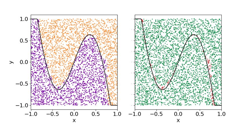
6.4 Classification of non-convex figures
for a single-qubit classifier trained with the weighted
As a final benchmark, we propose the classification of fidelity cost function. It requires four layers to learn
a non-convex pattern. In particular,pwe classify the that there are three concentric patterns and the ad-
points√of an annulus with radii r1 = 0.8 − 2/π and dition of more layers adjusts these three regions.
r2 = 0.8. We fix three classes: points inside the
small circle, points in the annulus and points outside 6.5 Comparison with classical classifiers
the big circle. So, besides it being a non-convex clas-
sification task, it is also a multi-class problem. A sim- It is important to check if our proposal is in some
pler example, with binary classification, can be found sense able to compete with actual technology of su-
Accepted in Quantum 2020-01-27, click title to verify. Published under CC-BY 4.0. 12You can also read