Using Payments Data to Nowcast Macroeconomic Variables During the Onset of COVID-19
←
→
Page content transcription
If your browser does not render page correctly, please read the page content below
Staff Working Paper/Document de travail du personnel —
2021-2
Last updated: January 21, 2021

Using Payments Data to
Nowcast Macroeconomic
Variables During the
Onset of COVID-19
by James T. E. Chapman and Ajit Desai

Funds Management and Banking Department
Bank of Canada, Ottawa, Ontario, Canada K1A 0G9

jchapman@bank-banque-canada.ca, ADesai@bank-banque-canada.ca

Bank of Canada staff working papers provide a forum for staff to publish work-in-progress research independently
from the Bank’s Governing Council. This research may support or challenge prevailing policy orthodoxy. Therefore, the
views expressed in this paper are solely those of the authors and may differ from official Bank of Canada views. No
responsibility for them should be attributed to the Bank.

ISSN 1701-9397                                                                               ©2021 Bank of Canada
Acknowledgements
We would like to thank Andre Binette, Narayan Bulusu, Shaun Byck, John Galbraith, Anneke
Kosse, Maarten van Oordt, Rodrigo Sekkel, and seminar participants at the Bank of Canada,
Vienna Workshop on Economic Forecasting 2020, and Banca d'Italia and Federal Reserve Board
Joint Conference on Nontraditional Data & Statistical Learning with Applications to
Macroeconomics for their suggestions. We also thank Adam Epp and Poclaire Kenmogne for
excellent research assistance.

                                            i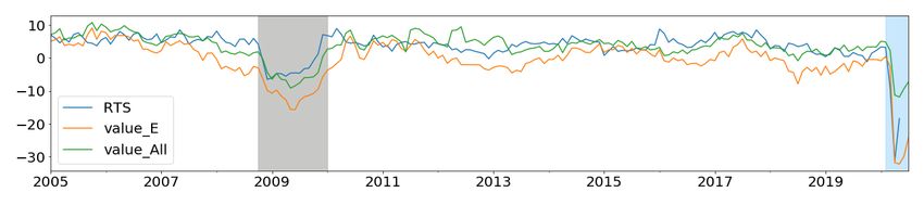
Abstract
The COVID-19 pandemic and the resulting public health mitigation have caused large-scale
economic disruptions globally. During this time, there is an increased need to predict the
macroeconomy’s short-term dynamics to ensure the effective implementation of fiscal and
monetary policy. However, economic prediction during a crisis is challenging because of the
unprecedented economic impact, which increases the unreliability of traditionally used linear
models that use lagged data. We help address these challenges by using timely retail payments
system data in linear and nonlinear machine learning models. We find that compared to a
benchmark, our model has a roughly 15 to 45% reduction in Root Mean Square Error when
used for macroeconomic nowcasting during the global financial crisis. For nowcasting during
the COVID-19 shock, our model predictions are much closer to the official estimates.

Bank topics: Econometric and statistical methods, Payment clearing and settlement systems
JEL codes: C53, C55, E37, E42, E52

                                              ii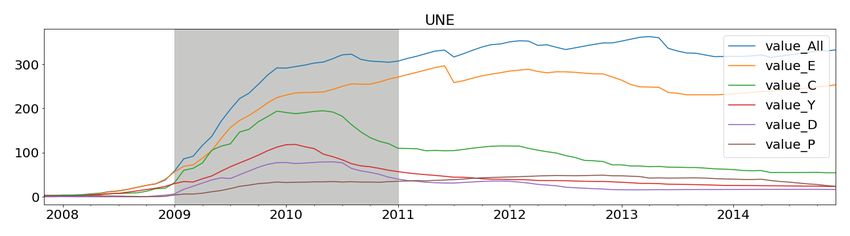
1    Introduction

The spread of COVID-19 globally has caused large-scale loss of life and unprecedented eco-
nomic damage (McKibbin and Fernando 2020). Governments worldwide have responded to
these shocks on a multitude of dimensions, including public health measures, fiscal stimulus,
and monetary policy (Bank of Canada 2020; Baldwin and Mauro 2020). Monetary policy de-
cisions in particular require an understanding of the current state of the economy; However,
estimating the current state of the economy – often referred to as economic nowcasting – is
difficult for two reasons: (a) delay, i.e., most of the official estimates of economic indicators
are released with a substantial lag, and (b) uncertainty, i.e., these indicators undergo mul-
tiple revisions later, sometime years after their first release (Giannone et al. 2008; Banbura
et al. 2010).
    Traditionally, policy institutions have used lagged macro variables in linear models to
predict the current state of the economy. Such approaches are useful in normal circumstances.
However, during economically stressed periods, macroeconomic nowcasting is challenging
because of the unprecedented economic impact and the speed of policy changes. During
such times – as we move forward into this unfamiliar world – traditional lagged data and
linear regressive models used for predictions become unreliable due to their slow response
and limited ability to capture sudden and large effects.
    To address these issues, this paper aims to predict the current state of the economy
using retail payments system data in linear and nonlinear machine learning (ML) models.
Canadian retail payments data capture numerous types of transactions, such as consumers’
income and expenditures, business-to-business payments, and Canada’s government transfer
payments. In the past, it has been shown that such data carry timely information about
the economy and they are useful for predictions (Galbraith and Tkacz 2007; Carlsen and
Storgaard 2010; Barnett et al. 2016; Duarte et al. 2017; Galbraith and Tkacz 2018; Raju and
Balakrishnan 2019; Aprigliano et al. 2019), more so during crisis periods such as COVID-19.
For example, in the recent paper by Chetty et al. (2020), the authors illustrate how private
                                            1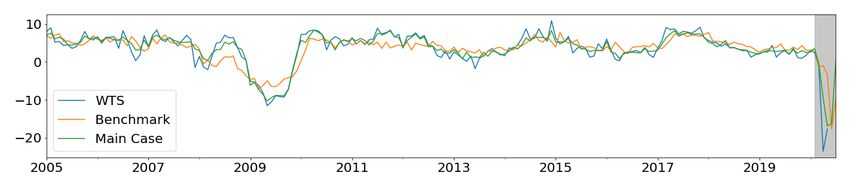
sector spending data can help rapidly identify the origins of economic crises. Similarly,
in Bounie et al. (2020), the authors demonstrate changes in consumer response to a severe
economic shock due to COVID-19 using card transactions data in France.
   We use a high-frequency payments dataset that consists of the settlement of multiple
payments instruments. Our dataset is much more comprehensive than the data sets used
in Galbraith and Tkacz (2018); Chetty et al. (2020); Bounie et al. (2020). Furthermore,
our data come from the main settlement system for retail payments in Canada, so it has
no sampling error. Therefore, due to its timeliness and comprehensiveness, it is an ideal
candidate for macroeconomic nowcasting during a crisis.
   We employ ML models such as the elastic net, support vector machines, random forest,
and gradient boosting to efficiently leverage the broad cross-section of different payments
instruments simultaneously (Zou and Hastie 2005; Burges 1998; Breiman 2001; Friedman
2001). These models are flexible, so they can help us capture nonlinear interactions between
the predictors and macro indicators (Richardson et al. 2018). This is important in the current
situation since the economic effects of COVID-19 are sudden and large.
   As a benchmark, our analysis indicates that during the global financial crisis, these
payments data in conjunction with ML models (in this case, gradient boosting) improve
prediction accuracy by up to 45% over a benchmark linear time-series model. We also
document that the nowcasts from our model are currently much closer to May and June
2020 official estimates than this benchmark model. Our benchmark model includes lagged
macro variables and the high-frequency Canadian Financial Stress Indicator (CFSI) (Duprey
2020) in a linear regression model.
   Historically, econometricians have used new data or developed new techniques to better
understand the current state of the economy (Giannone et al. 2008; Ghysels et al. 2007;
Bok et al. 2018; Kapetanios and Papailias 2018). The new data sources have spurred the
development and use of different econometric techniques. One popular approach involves
dimension reduction of a broad cross-section of time series: for example, the nowcasting
                                              2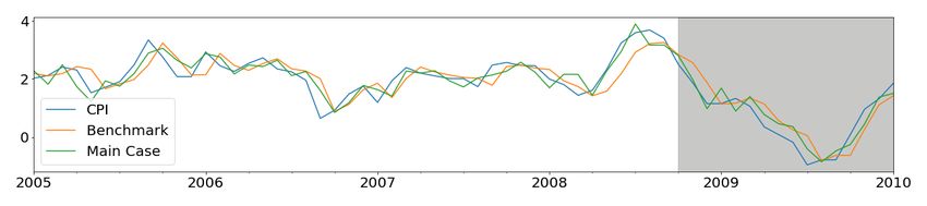
dynamic factor model (DFM) of Giannone et al. (2008). Another approach involves using
different frequencies of data to construct a better forecast, such as mixed-data sampling
(MIDAS) models developed by Ghysels et al. (2007). Although DFM performs slightly
better than the MIDAS model, both are shown to be competitive in predicting Canada’s
GDP by Chernis and Sekkel (2017).
    Recently, econometricians have started exploiting non-traditional, high-frequency, and
large-scale data sets, such as the financial market data, Google search data, and satellite
data for economic nowcasting and forecasting (Choi and Varian 2012; Andreou et al. 2013;
Li 2016; Donaldson and Storeygard 2016; Koop and Onorante 2019; Buono et al. 2017).
Non-traditional and large-scale datasets sometimes do not fit into the traditional economet-
ric models. Therefore, researchers have begun exploiting ML-based prediction approaches.
For example, the articles by Einav and Levin (2014a,b) suggest that the ML approaches com-
plement the traditional econometric tools and are useful in extracting economic value from
non-traditional data sources. The articles by Chakraborty and Joseph (2017); Richardson
et al. (2018) suggest that the ML models generally outperform traditional linear model-
ing approaches in prediction tasks, and in some cases, the ML algorithms outperform the
commonly used econometric tools, such as DFM.1
    In addition, econometricians have used electronic transactions datasets that potentially
have information related to the economy. This makes intuitive sense since virtually all
exchanges of goods and services are paid and settled via some payment systems. In Verbaan
et al. (2017), the authors use debit card payments data for nowcasting Dutch household
consumption. In Galbraith and Tkacz (2018), the authors use point-of-sale debit and cheque
payments data to nowcast Canada’s GDP and retail sales. Similarly, in Aprigliano et al.
(2019), the authors use some of the data from Italy’s retail payments system for nowcasting
and forecasting.
    In this paper, we extend earlier work by Galbraith and Tkacz (2018); they use a subset
   1 A comprehensive review of the use of machine learning (ML) and big data for nowcasting and forecasting is

presented in the following articles (Hassani and Silva 2015; Kapetanios and Papailias 2018).
                                                      3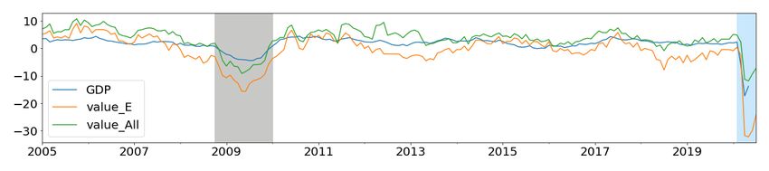
of the streams of payments data in our dataset to nowcast Canada’s GDP and retail sales
using an ordinary least squares model. In contrast, we use all settlement data from retail
payment systems and also use more flexible models to capture the large effects of the crisis.
Using all data is important to overcome a drawback of the previous study, i.e., payments
through particular instruments may rise or fall due to non-economic reasons (technological
advancements such as the decline of cheque usage). Using one or two payments instruments
in isolation could bias predictions. Our paper is also an extension of our earlier work on
payments data and ML for nowcasting (Chapman and Desai 2020), with the primary focus
being on the current crisis period.
    We proceed as follows. In section 2 we describe the retail payments system data. Section
3 provides a brief overview of the nowcasting methodology, followed by the results and
discussion in section 4. Finally, in section 5 we conclude our findings. Several appendices
provide details on the payments data and the ML-based nowcasting methodology employed
in this paper.

2     Retail Payments System Data

The vast majority of non-cash transactions require settlement to extinguish the debt be-
tween the buyer and the seller.2 In modern economies, this is typically accomplished via
a centralized payments system. In Canada, there are two systems operated by Payments
Canada that settle these transactions: the Automated Clearing and Settlement Systems
(ACSS) and the Large-Value Transfer System (LVTS). ACSS settles the majority of retail
and small-value payment items, and LVTS clears large-value payments between Canadian
financial institutions. In this paper, we focus on payments data from ACSS only. In 2019,
ACSS handled an average of 33 million payments items per day, with an average daily total
value of $29 billion.
    2 According
              to recent surveys, only 14% of physical retail sales by value settled with physical cash as opposed to
through a payment system (Henry et al. 2018).

                                                         4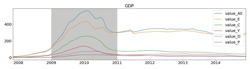
ACSS clears 24 types of payments instruments (referred to as streams). Broadly, these
streams can be categorized into two groups: electronic streams, which include, for example,
Automated Fund Transfer (AFT), Point-of-Sale (POS) Payments, Electronic Data Inter-
change (EDI), On-line payments, and Government Direct Deposit; and paper-based streams,
which incorporate Encoded Paper, Paper Remittances, Government Paper Items, etc.
    Over time since ACSS’s inception in 1999, some payments streams were discontinued,
some new streams were created, and some were merged; therefore, in this study, we use
transactions settled in 20 payments instruments. These streams account for the majority of
the payments settled in ACSS. Our data consist of the daily gross dollar amount, i.e., value,
and number of transactions, i.e., volume settled in those payments instruments.
    To overcome the effects of the sudden changes in the streams and to get a better rep-
resentation of payments flow, we merged a few streams which belong to similar categories
and settle related payments.3 This could help us to mitigate the non-stationarity effects
due to sudden changes in streams (primarily driven by technological advancements). Also,
to overcome the effects of consumers’ choice of payments, i.e., when they switch payments
method,4 we include the sum of all payments instruments in ACSS, Allstream, as a separate
series. This should assist us in getting the overall picture from ACSS and mitigating the
effects of a few unused streams. After these adjustments, we are left with 12 streams that
are listed in Table 1 along with a short description.5 We use both value and volume of each
stream; therefore, we have in total 24 series.
    The shares of many streams (in terms of value and volume of payments) have changed
over time. Due to their usability, electronic means of payments have become more common
than paper items. Most of these changes are primarily driven by technological advancements
leading to the inception and adoption of new payment instruments; however, an economic
crisis like COVID-19 can also influence the payments flow.
   3 See  Table 1 footnotes for the specifics of each adjustment performed.
   4 For  nowcasting, we are interested in capturing whether spending (or earning) has actually slowed (or stopped),
rather than switched payment method.
    5 Further details of the individual payments instruments are provided in Appendix A.

                                                         5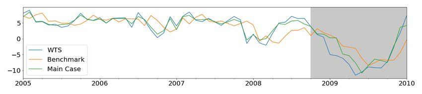
Table 1: ACSS payments streams used in this studya

ID     Label                          Short Description

C      AFT Credit                     Direct Deposit (DD): payroll, account transfers
D      AFT Debit                      Pre-authorized debit (PAD): bills, mortgages, utility
E      Encoded Paperb                 Paper bills of exchange: cheques, bank drafts, paper PAD
F      Paper Remittances              Corporate bill payments. Settles payments similar to Y-stream
G      Government Itemsc              Paper items: Government of Canada paper items
J      On-line Paymentsd              Electronic payments using a debit card through the internet
M      Government DD                  Recurring social payments: social security, tax refunds
N      Shared ABM Network Debit card payments to withdraw cash at ABM
P      POS Paymentsd                  Point-of-sale (POS) payments using debit card
X      EDI Paymentse                  Exchange of corporate-to-corporate payments
Y      EDI Remittances                Corporate electronic bill payments
All Allstream                         The sum of all payments streams settled in the ACSS
a   These eleven payments streams are representative of 20 payments instruments in the ACSS. There are a few
    more payments instruments; however, because they are not available for the entire time period we’re con-
    sidering in this paper, they are excluded from this study. The excluded streams are ABM Adjustments, ICP
    Regional Image Payment, and ICP Regional Image Returns. NOTE: Excluded streams collectively account for
    about 0.001% of the total value settled in the system. For further details on ACSS streams, refer to Appendix A.
b   Stream E is the sum of multiple streams settled separately in ACSS. It combines Encoded Paper (E), Large-
    Value Encoded Paper (L), and Image Captured Payments (O) streams and subtracts Image Captured Return
    (S), Unqualified (U), and Computer Rejects (Z) streams.
c   Stream G is the sum of multiple streams settled separately in ACSS. It incorporates Canada Savings Bond (B),
    Receiver General Warrants (G), and Treasury Bills and Bonds (H).
d   Value and volume of On-line Payments (J) and POS Payments (P) streams are obtained by subtracting On-line
    Returns (K) and POS Refund (Q) streams, respectively.
e   EDI: Electronic Data Interchange.

                                                        6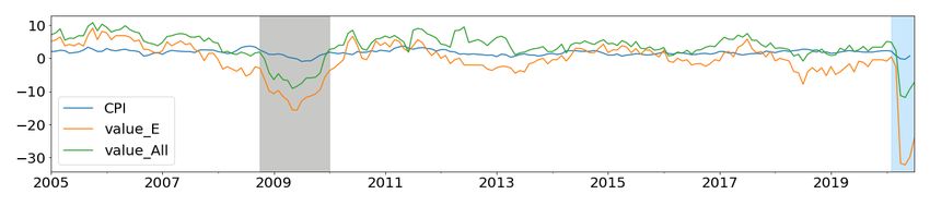
Figure 1: Shares of payments streams in terms of value (dollar amount) after making adjustments
outlined in Table 1. Historic period: Jan 1999 to July 2020, and latest period: April to July 2020.
NOTE: The shares of Shared ABM Network, Government Items, Paper Remittances, and On-line
Payments are < 0.4% for both the historic and latest periods. However, the Government Items
increased to 1.5% in the latest period.

Figure 2: Shares of payments streams in terms of volume (number of transactions) after making
adjustments outlined in Table 1. Historic period: Jan 1999 to July 2020, and latest period: April
to July 2020. NOTE: The shares of Paper Remittances, Government Items, EDI Payments, and
On-line Payments are < 0.3% for both the historic and latest periods.

                                                7
In Figure 1 and Figure 2, we compare the value and volume shares of each payments
stream using the entire dataset (historical data ranging from Jan 1999 to July 2020) with
the latest data, i.e., for the period ranging from April to July 2020. Historically, the En-
coded Paper stream has the highest value shares, followed by the AFT Credit, and the POS
Payments stream has the largest volume shares, followed by the Encoded Paper stream.
In recent months – fueled by social-distancing rules due to COVID-19 – the AFT Credit
value (primarily used for payroll) share has more than doubled, and that of Encoded Paper
stream shares has been halved, compared to the historical shares. Similarly, the transactions
value settled in Government Direct Deposits stream (which settles government social security
payments) has increased four times. This increase in flow is likely due to the Canada Emer-
gency Response Benefit (CERB) payments to provide financial support to Canadians who
are directly affected by COVID-19. Similar effects are observed in the volume of payments.
For example, the POS Payments volume shares have increased by 7 percentage points, and
Encoded Paper volume shares have decreased by 11 percentage points.
ACSS payments capture numerous types of transactions from both sides of macroeco-
nomic accounts: for example, consumers’ income and expenditures. It includes, for instance,
payrolls and government social payments from the income side; and bills, mortgages, utilities,
donations, and cash withdrawals from the expenditure side. ACSS also includes business-
to-business bill payments in EDI and Canada’s government spending in Government Paper
Items. Therefore, this variety, timeliness, and the lack of errors in the ACSS dataset make
it a rich economic information source. Thus, it is an ideal candidate for high-frequency
economic monitoring and macroeconomic nowcasting (Galbraith and Tkacz 2007, 2018).
Note that our dataset does not include some of the payments instruments which are not
settled through the ACSS, such as credit card and e-transfer payments.6 However, Galbraith
and Tkacz (2018) concluded that the credit card payments data in Canada does not add
6 In2019, credit card payments accounted for about 6.2% in value and 31.1% in volume of total retail transactions
in Canada. Similarly, e-transfer payments accounted for 1.5% in value and 2.5% in volume (Paturi and Chiron 2020).
8any value in nowcasting GDP and retail sales.7 Furthermore, our dataset does not include
on-us transactions where both sender and receiver have an account with the same financial
institution; therefore, such transactions do not need to be settled in ACSS. However, their
shares are small and hence might not drastically influence our analysis.8
2.1 Effects of COVID-19 Shock on Payments Streams
The COVID-19 pandemic is having an unprecedented economic impact on the Canadian
economy. Before COVID-19 struck Canada, the economy had been operating close to po-
tential for nearly two years (Bank of Canada 2020). However, most economic activities have
been reduced substantially due to the COVID-19 shock and the public health response to it.
These effects are directly visible through some of the ACSS payment streams.
ACSS data, which are available daily, can be used for high-frequency economic monitor-
ing.The effects of most of the economic activities of consumers, corporations, and government
can be observed daily using these streams. This is important for policymakers in economi-
cally stressed periods to quantify the immediate effects of such extreme events.
In Figure 3, we present daily value and volume series for three payments streams, namely,
shared ABM Network, POS Payments, and Government Direct Deposit.9 The effects of
COVID-19 shock are evident through these time series. Both values and volumes of ABM
Network and POS Payments fell starting in mid-March 2020, and when the full effects of
the pandemic hit in April, both value and volume reached their lowest levels. Starting in
mid-May 2020, both ABM and POS streams show signs of recovery. By the end of May,
the POS stream had recovered to the pre-COVID level; however, the ABM stream is still
recovering slowly. Similarly, the Government Direct Deposits stream shows the increased
7 Note that in Galbraith and Tkacz (2018) the authors used a short sample size in their analysis of credit card data.
The results could be different for a larger sample size.
8 On-us payments amount to roughly 20% more than those settled in ACSS. The values of on-us transactions differ
by payments instrument; for instance, in Encoded Paper, it is about 25%, and in POS Payments, it is about 16% (Paturi
and Chiron 2020).
9 We select these streams because the effects of COVID-19 shock are clearly visible in these streams and cover both
earnings and spending.
9flow during the same period, confirming the effects of social security payments, probably
under CERB, launched during the onset of COVID-19.
Figure 4 compares the monthly aggregated value and volume of Encoded Paper, POS
Payments, and Allstreams, respectively.10 A sudden and massive drop in these streams’
values and volumes in April 2020 highlights the severity of COVID-19’s effect on the economy.
Compared to the same period in 2019, the Encoded Paper stream value fell by 33%, and
volume dropped by 39%. Similarly, we observe a 32% and 41% drop in value and volume
of POS Payments as well as 15% and 27% decline in value and volume respectively for all
payment streams via the Allstream variable.
The higher drop in volumes compared to values in these streams indicates that consumers
choose to spend in bulk, i.e., they avoid multiple visits to marketplaces to reduce the risk of
catching COVID-19. Starting in June 2020, the POS stream has recovered to pre-COVID
level; however, the Encoded Paper stream has yet to recover. The Allstream value and
volume show that ACSS is recovering fast; but, it had not entirely recovered by July 2020.
2.2 Payments Data for Macroeconomic Nowcasting During a Crisis
The crux of the problem of nowcasting during a crisis is that most of the official estimates
of macroeconomic indicators are released with a substantial delay. For instance, GDP in
Canada is released with a delay of eight weeks. Furthermore, these indicators can undergo
revisions sometimes years after their first release, highlighting the uncertainty of the mea-
surement. Therefore, it is valuable to provide current-period estimates of these indicators
using more timely available information: in this case, payments data from the ACSS.
During a rapid crisis such as COVID-19, macroeconomic predictions are difficult because
of the large and unprecedented economic impact.11 This could undermine the use and relia-
10 We select these streams because the Encoded Paper stream accounts for the highest value share, POS Payments
stream accounts for the largest volume shares, and Allstream is an indicator of the entire value and volume of transac-
tions settled in ACSS.
11 The unemployment rate soared to 13% in Apr 2020 as the full force of the pandemic hit, compared with 7.8% in
Mar 2020 (Statistics Canada. Table 14-10-0287-01, monthly, seasonally adjusted).
10Figure 3: Selected payments streams’ value (blue) and volume (orange) at daily levels for the
period before and during the COVID-19 crisis.
11Figure 4: Comparison of the monthly aggregated and seasonally adjusted Encoded Paper (E), POS
Payments (P) and Allstream (All) value and volume streams for the last three years. Highlighted
(in gray) is the ongoing COVID-19 period.
12Table 2: Delay period for official estimates of key
macroeconomic indicators in Canada.
ID Macroeconomic Variable Delay Period
GDP Gross Domestic Product 8 weeks
RTS Retail Trade Sales 6 weeks
WTS Wholesale Trade 6 weeks
HPI New House Price Index 6 weeks
CPI Consumer Price Index 2 weeks
UNE Unemployment 1 week
bility of traditional lagged data and linear models used for nowcasting, which typically have
at least an implicit assumption that the economy is in some sort of stationary equilibrium.
Therefore, non-traditional models and higher frequency data in real time are needed.
For demonstration, we use the macroeconomic indicators listed in Table 2 as target
variables12 for nowcasting using ACSS payments data. Like other macroeconomic time
series, ACSS streams have a strong seasonal component. We adjust all series (both value
and volume) for seasonality using the X-13 ARIMA tool (X13 Reference Manual 2017).13
The year-over-year (YOY) growth rates of the seasonality adjusted payments series are used
to predict the similarly adjusted YOY growth rates of macroeconomic indicators.
Pairwise correlations between YOY growth rates of the seasonality adjusted macroeco-
nomic variables and selected payments streams are listed in Table 3. These indicate that
most of the ACSS streams have a strong correlation with macroeconomic indicators. The All-
stream and Encoded Paper values are strongly correlated to the most macro indicators. AFT
Credit and POS Payments have a high correlation with Retail Trade Sales (RTS), Wholesale
Trade Sales (WTS), House Price Index (HPI), and Consumer Price Index (CPI). Shared
12 Seasonally adjusted monthly GDP, RTS, WTS, HPI, CPI, UNE are obtained from Statistics Canada Tables 36-10-
0434-01, 20-10-0008-01, 20-10-0074-01, 18-10-0205-01, 18-10-0006-01, and 14-10-0287-01, respectively.
13 Seasonality adjustments are performed because official macro indicators are released with similar adjustments.
13ABM values and volume are strongly correlated with GDP, WTS, and Unemployment.
Table 3: Pairwise correlations between YOY growth rates of the seasonality adjusted
macroeconomic variables and a few selected payments streams.*
E-value All-value N-value N-volume P-value All-volume C-value
GDP 0.85 0.81 0.81 0.74 0.67 0.67 0.59
RTS 0.80 0.70 0.77 0.73 0.76 0.71 0.62
WTS 0.83 0.82 0.66 0.56 0.54 0.52 0.59
HPI 0.53 0.57 0.27 0.15 0.51 0.11 0.64
CPI 0.51 0.22 0.44 0.30 0.38 0.31 0.56
UNE -0.87 -0.79 -0.85 -0.78 -0.68 -0.70 -0.55
*1 Correlations are calculated for the period Jan 2005 to July 2020.
*2 Payments streams: All-Allstream, E -Encoded Paper, N - Shared ABM Network, C - AFT Credit, D -
AFT Debit, P - POS Payments, and Y - EDI Remittances.
*3 Macroeconomic variables: GDP - Gross Domestic Products, RTS - Retail Trade Sales, WTS - Whole-
sale Trade Sales, CPI - Consumer Price Index, HPI - House Price Index, and UNE - Unemployment.
Value is the dollar amount, and volume is the number of transactions.
*3 Payment streams are arranged in ascending order of their correlation with GDP, and the order is kept
constant for all other macro variables.
The YOY growth rates of Allstream and Encoded Paper values are plotted with YOY
growth rates of GDP, RTS, WTS, HPI, CPI, and Unemployment (UNE) in Figure 5. To
get a sense of the importance of the payments data during a crisis, we highlight the growth
rates of Allstream and Encoded Paper during the 2008 global financial crisis (in gray) and
COVID-19 shock (in blue).
During this period, the decline and rebound in growth rates of these payments streams go
hand in hand with macroeconomic indicators. This is a good indication of the economic value
associated with these payments streams during the crisis period. Similarly, both Allstream
and Encoded Paper values’ growth rates show a dramatic drop in Apr 2020, showing the con-
sequences of the COVID-19 shock. This implies that payments data, which is available daily,
could be exploited to quantify the effects of the COVID-19 shock on crucial macroeconomic
indicators.
14Figure 5: Growth rate comparisons of macro variables with Encoded Paper (E) and Allstream
(All). Highlighted in gray is the global financial crisis period; blue shows the ongoing COVID-19
period.
153 Methodology
To exploit non-traditional and large-scale data sources, researchers have recently begun uti-
lizing ML models for economic prediction. The ML models are shown to efficiently handle
wide- and large-scale data and can manage collinearity. Furthermore, they are demonstrated
to methodically capture non-linear interactions between the predictors and the target vari-
able. However, there are some challenges in using ML models for macroeconomic predic-
tions (Einav and Levin 2014a,b; Chakraborty and Joseph 2017).
The use of ML models sometimes leads to a loss of interpretability and the problem of
overfitting. These models also demand large-scale data, which is often hard to get in the
context of macroeconomic prediction (Chakraborty and Joseph 2017). However, the ML
models employed in this paper, such as elastic net regularization, support vector regression,
random forest, and gradient boosting, are interpretable up to a certain extent (Zou and
Hastie 2005; Burges 1998; Breiman 2001; Friedman 2001). Also, the problem of overfitting
can be mitigated using cross-validation techniques (Hastie et al. 2009; Friedman et al. 2001).
Nonetheless, ML models are useful in cases when the emphasis is on improving prediction
accuracy – which is the primary focus of this paper. Richardson et al. (2018) shows that some
of the ML models outperform the commonly used nowcasting approaches, such as DFM, in
nowcasting New Zealand’s GDP. Below we briefly discuss the nowcasting models employed
in this paper. This section borrows from Chapman and Desai (2020). The interested reader
is encouraged to read that paper, where we provide a fuller exploration and comparison of
the models referred to here and references therein.
Consider a set X = {x1 , x2 , . . . , xM } of M attributes (sometimes called predictors or inde-
pendent variables) and a target y (dependent variable), each with N data points. This can
be represented as a dataset (X, y) where X is of size N × M and y is a vector of size N × 1.
Let us denote ŷ as the predicted target, which can be obtained using an OLS model as
ŷ(X, w) = Xw, (1)
16where w is a vector of unknown coefficients (weights) of size M × 1. In OLS, we fit the linear
model of the form given in Equation 1, and the objective is to minimize the residual sum of
squares between the observed values y and the predicted values ŷ of the target,
min ky − ŷ(X, w)k2 , (2)
w 2
where k.k∗ is L∗ norm. Such linear models have proven to be a valuable and straightforward
model for prediction due to the Gauss-Markov Theorem (if the underlying data satisfies
a few assumptions about the distributions of the error) and many years of practical use.
However, when some of the predictors are correlated, the OLS estimates become highly
sensitive to random errors in the target. Also, OLS is susceptible to the outliers in the data
and, importantly, can only model relationships linear in the parameters w. Therefore, it
generally does not perform well on large and complex datasets (Hastie et al. 2009).
We also employ some of the recently popularized parametric and non-parametric ma-
chine learning approaches such as elastic net (Zou and Hastie 2005), support vector ma-
chines (Smola and Schölkopf 2004), random forest (Breiman 2001; Liaw and Wiener 2002),
and gradient boosting (Friedman 2001). For each considered model there are many variations
proposed in the literature; however, we have focused on the basic version of each model. We
give a high-level description of each below.14 .
The elastic net (ENT) is a regularized linear regression model. Here the objective is
similar to that of the OLS in Equation 2 with the addition of L1 and L2 penalties on how large
the sum of the parameters w can get.15 In an elastic net regression, the combination of L1 and
L2 penalties allows for learning a sparse model while encouraging grouping effects, stabilizing
regularization paths, and removing limitations on the number of selected variables (Zou and
Hastie 2005).
Support vector regression (SVR) is another model useful for the problems with multiple
14 For further details on these models, refer to Appendix B
15 A regression model that uses only the L1 penalty is a Lasso regression, and a model that uses only the L2 penalty
is a Ridge regression (Hastie et al. 2009; Zou and Hastie 2005).
17predictors. It uses a very different objective function compared to the OLS or ENT. The
SVR is based on support vector machines. These are algorithms whose task is to find a
hyperplane that separates the entire training dataset into, for example, two groups by using
a small subset of training points (called support vectors). In the case where there is no
such hyperplane, it is modified to minimize the number of misclassified points in every
region (Burges 1998; Smola and Schölkopf 2004).
Another popular approach is random forest (RF) regression. It is a decision tree–based
ensemble learning method built using a forest of many regression trees. It is a non-parametric
method and hence approaches the multicollinearity problem slightly differently than para-
metric approaches such as OLS or ENT. Random forest is also a bagging (bootstrap aggre-
gation) approach, i.e., each tree is independently built from a subset of the training dataset.
Each sample could randomly select a subset of features from the available set or the entire
features set. The final prediction is performed by averaging the predictions of all regression
trees (Breiman 2001; Liaw and Wiener 2002).
Similar to the random forest, gradient boosting (GB) regression is a tree-based non-
parametric ensemble learning approach. However, unlike random forest, this approach is
based on boosting in which a sequence of weak learners (for example, small decision trees)
are built on a repeatedly modified version of the training dataset. The data modification at
each boosting interaction consists of applying weights to each of the training samples, and
for successive iterations, the sample weights are modified (Friedman 2001).
3.1 Model Training and Cases Specifications
In the implementation of the above-discussed methods, we use the expanding window ap-
proach. We first divide the dataset into two subsets: a training set and a testing set. Next,
part of the training set, i.e., a validation set, is kept aside for model tuning and cross-
validation.16
16 Refer to Figure 10 in Appendix D for schematic representation and further description.
18We train the models in two steps. During the first step, we use the training and validation
sets. For each iteration (or fold) of the expanding window, we increase the training sample
by one period and then predict the next period from the validation set. At the end of this
step, i.e., when we finish iterating over the validation set, a few selected hyperparameters for
each of the models are tuned using cross-validation.17 In the second step, the tuned models
are used for prediction by reutilizing the expanding window approach over the training and
testing set. For the out-of-sample model evaluation, we use Root Mean Square Error (RMSE)
as the key performance indicator.18
As a benchmark, we first employ a linear regression model using OLS and then utilize
more sophisticated ML models discussed in section 3. The time horizon for nowcasting t + 1
is based on the payments data availability. For example, if we use payments data available
at t and first available lag (t − 2 for GDP), then the model F can be specified as
[ t+1 = F (GDPt−2 , Paymentst ).
GDP (3)
In the naive benchmark, we use an autoregressive (AR) model using the first available
lagged macro variable. For GDP, retail, and wholesale trade sales, which are released with
two months’ lag, we use the second lag; and for all other macro variables, we use the first
lag, as they are available with less than one month lag. For example, to nowcast July’s GDP
growth rates on August 1, we use official estimates of May (second lag). Similarly, we use
June’s official estimates to nowcast July’s unemployment growth rates.
In the benchmark (or the base case), we use predictors from the naive case along with
the Canadian Financial Stress Indicator (CFSI) in the OLS model. For example, to nowcast
July’s GDP on the first day of August, we use CFSI for July’s and May’s GDP growth
rate. The CFSI is a newly created composite measure of systemic financial market stress
for Canada. It is available immediately and is shown to track the economic crisis (Duprey
17 We choose the parameters which give the best performance (lowest RMSE) on both training and validation sets.
18 All models utilized here are employed using Scikit-learn: Machine Learning in Python (Pedregosa et al. 2011).
192020). The CFSI is constructed using data from multiple market segments.19 Therefore, it
is a useful predictor to nowcast macroeconomic indicators and hence is used as a benchmark
to compare information gain using payments data.
In the main case of interest, along with the predictors specified in the base case above,
we use the payments streams listed in Table 1. For example, to nowcast July’s GDP on the
first day of August (at t + 1), we use payments data and CFSI for July (at t) and the GDP
growth rate of May (at t −2).20 The model selection for the main case of each macroeconomic
variable is performed using the following steps:
1. First, we compute prediction scores for payments streams for the selected macro vari-
able using univariate linear regression tests (see Appendix C for further details).
2. Next, we arrange payments stream in the descending order of their scores and incor-
porate one stream at a time from that list for the prediction.
3. We repeat steps 1 and 2 for each regression method discussed in section 3 and get the
in-sample training and out-of-sample testing RMSEs for all cases.
4. Finally, we select the best model, i.e., the model with least in-sample training and
out-of-sample testing RMSEs, to report the nowcasting results.
4 Results and Discussion
We present the results of nowcasting for the cases specified above. Situations of severe shock
are natural areas in which our data and techniques are particularly useful. Therefore, we
employ them to study the economic crisis periods. We first demonstrate the usefulness of
19 CFSI is computed using the data from the following seven market segments: the equity market, the Government
of Canada bonds market, the foreign exchange market, the money market, the bank loans market, the corporate bonds
market, and the housing market.
20 Traditionally, predictions are performed at multiple time horizons, for example, extending from the start of the
month of interest until a day before the official release (Giannone et al. 2008; Galbraith and Tkacz 2018). However,
in this paper, we focus on the current period, which is critical for policymakers during crisis. Also, payments data are
shown to add the most value at nowcasting horizon, i.e., at t + 1 (Galbraith and Tkacz 2018; Aprigliano et al. 2019).
20ACSS payments data during the global financial crisis as a test case. Next, we use payments
data to nowcast macroeconomic indicators for the current COVID-19 period.
ACSS payments data used for these exercises range from Jan 2005 to Jul 2020 (p = 187
sample points). YOY growth rates nowcasting of various macro variables for the benchmark
and the main cases are performed. The results of these exercises are discussed in the following
sections.
4.1 Global Financial Crisis
In this case, the in-sample training period is Jan 2005 to Oct 2008 (p = 46), and the out-of-
sample testing period is Nov 2008 to Jan 2010 (p = 14), i.e., the 2008 financial crisis period
with significantly low growth rates. In Table 4, we compare the nowcasting performance
(in terms of RMSE) of the only best-performing ML model (from the list of the following
models: elastic-net, support vector machines, random forest, and gradient boosting) on the
main case data with the OLS on main case data and benchmarks.
ACSS payments data provide significant reductions in nowcasting RMSE for most of the
macroeconomic variables considered in this paper. The information gain using payments
data is higher for the macro variables, which have a higher delay period. For instance, we
get 50 to 60% reduction in RMSE over AR model and 38 to 44% RMSE reductions over
benchmark case in nowcasting GDP, retail trade sale, and wholesale trade sale (which are
delayed by six to eight weeks).
Comparatively, the information gain using payments data is slightly lower for the macro
variables, which have a shorter delay period. For instance, we get about 20 to 50% reduction
in RMSE over AR model and 12 to 21% reductions in RMSE over benchmark in nowcasting
unemployment, CPI, and HPI (which are delayed by only a week or two). Except for CPI
and HPI, all other main case predictions are statistically significant for the Diebold-Marino
test using the benchmark.21
21 We recognize that Diebold-Mariano test has poor finite-sample properties; however, we use it to be comparable
21It is worth noting that the major gains in nowcasting accuracy are achieved by using
payments data, i.e., we get 10 to 30% reduction in RMSE when payments data is used in
the OLS model. However, the ML models contribute to increasing prediction accuracy by 3
to 20% across all targets.
In nowcasting GDP and retail trade sale and wholesale trade sales, the gradient boosting
regression (a non-parametric and non-linear model) performs better than other models con-
sidered in this paper. The linear and parametric models, such as support vector regression
and elastic net, perform slightly better in nowcasting CPI, HPI, and unemployment. How-
ever, overall the gradient boosting model gives the consistently better performance across
all targets. This is probably due to its ability to efficiently handle multiple predictors and
capture sudden and large changes in interaction between the predictors and target variables
during economic crisis periods.
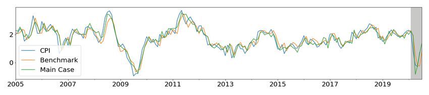
Visual comparisons of in-sample and out-of-sample predictions are depicted in Figure 6.
In all cases, including the payments data provides downturn and recovery indications that
are much better than the benchmark case in both in-sample and out-of-sample periods. We
conjecture that this is due to the new information provided by the payments data and the
flexible ML models that allow this data to provide better predictions.
In the prediction of almost all of the targets, the Allstream value and Encoded Paper value
scores22 highest among the payments steams, and they are identified as the most important
streams for macroeconomic nowcasting. In the case of GDP nowcasting, Allstream, Encoded
Paper, ABM Network, and AFT Credit values are more useful. Similarly, for RTS growth
rate nowcasting, along with the Allstream and Encoded Paper values, POS Payments, AFT
Credit, and AFT Debit values are more beneficial.
with similar papers where it has been used, for example (Chernis and Sekkel 2017; Aprigliano et al. 2019).
22 See Figure 9 in Appendix C for details on prediction scores for selected predictors.
22Table 4: Global financial crisis: RMSE on testing period for seasonally adjusted YOY
growth rate nowcasting of macro variablesa
Targetb ARc Benchmarkd Main-OLSe Main-MLf RMSE Reduction (%)g
GDP 1.63 1.18 0.73** 0.66h** 44
RTS 5.12 4.12 3.32** 2.54h*** 38
WTS 5.74 4.73 3.67* 2.76h*** 42
CPI 0.61 0.54 0.49 0.47i 12
HPI 0.67 0.39 0.34 0.33i 16
UNE 6.86 6.21 5.08* 4.90i* 21
a In-sample training period: Jan 2005 to Oct 2008 (p = 46) and out-of-sample testing period: Nov 2008
to Jan 2010 (p = 14). Note that the seasonality adjustment of the payments streams is performed for the
sample up to Jan 2010, i.e., including the test set.
b GDP-Gross Domestic Product, RTS-Retail Trade Sales, WTS-Wholesale Trade Sales, CPI-Consumer
Price Index, HPI-New House Price Index, and UNE-Unemployment. Note, we use the latest release of
these targets. It is more appropriate for such exercises to use the first-release; however, we do not have
the historic (real-time releases) data for some of these macro variables.
c Autoregressive model using the first available lagged macro variable (for GDP, RTS, and WTS second
lag and others first lag).
d For benchmark, we use OLS with CFSI and the first available lagged macro variable.
e For the main-OLS case, we use payments data along with the predictors in the benchmark case in the
OLS model.
f For the main-ML case, we use payments data along with the predictors in the benchmark case and only
show RMSE of the best-performing models chosen from the list of the following models: elastic net,
support vector machines, random forest, and gradient boosting.
g Percentage reduction in RMSE over benchmark using main ML model.
h Gradient boosting regression model performs the best, giving an additional 10 to 20% reduction over
OLS with the main case, i.e., when payments data is included. These indicate the RMSE reductions due
to ML models over OLS. Also, for gradient boosting, we explore and tune the following hyperparame-
ters: number of estimators (trees), maximum depth of each estimator, and learning rate.
Refer to Appendix B, C, and D for additional details on the model and tuning procedure.
i Support vector regression model performs the best, giving an additional 3 to 5% reduction over OLS
with the main case. For SVR model, we explore and tune the following hyperparameters: kernel type
and regularization parameter value.
*, **, *** denote statistical significance at the 10, 5, and 1% level, respectively, for the Diebold-Marino test
using the benchmark.
23Figure 6: Comparison of main case nowcasts during global financial crisis with the benchmark.
The in-sample training period is Jan 2005 to Oct 2008 and the out-of-sample testing period is Nov
2008 to Jan 2010 (highlighted in gray).
244.2 Covid-19 Shock
In this section, we present the results of macroeconomic nowcasting for the ongoing COVID-
19 period. For this case, we have a longer in-sample training period, i.e., Jan 2005 to Mar
2020 (p = 183), compared to the previous case. The trained models’ performance is examined
on the out-of-sample testing period ranging from Apr to Jul 2020. Since the testing sample
is tiny and our primary focus is on the crisis period, we select the best-performing model on
the global financial crisis for predictions (i.e., the models used for predictions in Table 4).
The predictions for May, Jun, and Jul 2020 are presented in Table 5.
For May 2020, our model predictions using payments data are much closer to the offi-
cially released values compared to the benchmark. In this case, the benchmark model could
correctly predict the sign (which is straightforward due to sharp drops in target values), but
the actual predictions fall short of official values. For this period, the nowcasting of macro
variables that have higher delay periods, such as GDP, RTS, and WTS, are more accurate
than those with shorter delay periods (CPI, HPI, and UNE). For Jun and Jul 2020, our model
predicts faster recovery of all macro variables. This is in line with the information seen in
most payments streams showing signs of recovery starting in Jun 2020. In contrast, the
benchmark model predicts recovery at a much lower rate. Note that the official estimations
of all macro variables for July 2020 will be available on Oct 1, 2020.
Employment is the hardest hit by COVID-19, and our model predicts that YOY growth
rates of unemployment increased by 80%, 74%, and 63% in May, Jun, and Jul 2020, re-
spectively. Model prediction falls short of the officially released estimates for that period;
however, our model performs much better than the benchmark model, which could not
capture the drastic effects of COVID-19 shock on unemployment. Similarly, our model per-
formance is more reliable than the benchmark of CPI and HPI but falls short of actual
predictions in May and June 2020. According to our model predictions, YOY growth rates
of CPI and HPI for July 2020 will be 1.37 and 1.46. The visual comparisons of in-sample
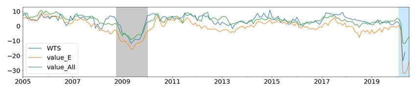
and out-of-sample predictions are depicted in Figure 7. In all cases, including the payments
25Table 5: COVID-19 Shock: Seasonally adjusted YOY growth rate predictions for May to July 2020.a
May 2020 Predictions Jun 2020 Predictions Jul 2020 Predictionse
Targetb Official Benchmarkc Maind Official Benchmark Main Benchmark Main
GDP -13.8 -5.81 -17.1 NA -14.6 -13.6 -6.47 -2.97
RTS -18.4 -7.58 -25.2 NA -20.8 -9.89 -5.96 1.58
WTS -17.7 -3.32 -17.9 NA -17.8 -14.8 -9.60 -0.71
CPI -0.29 -0.19 -0.24 0.73 -0.23 0.68 0.77 1.37
HPI 1.06 0.53 0.57 1.26 0.86 1.15 1.15 1.46
UNE 139.7 8.87 78.3 118.4 10.11 72.1 7.98 62.6
a In-sample training period: Jan 2005 to Mar 2020 (p = 183) and out-of-sample testing period: Apr to Jul 2020
(p = 4). Note that the seasonality adjustment of the payments streams is performed for the sample up to July 2020,
i.e., including the test set. Also, since the test sample is tiny, we do not provide out-of-sample RMSEs.
b GDP-Gross Domestic Product, RTS-Retail Trade Sales, WTS-Wholesale Trade Sales, CPI-Consumer Price Index,
HPI-New House Price Index, and UNE-Unemployment. Note, we use the latest release of these targets.
c For the benchmark, we use OLS with CFSI and the first available lagged macro variable (for GDP, RTS, and WTS
second lag and others first lag).
d For the main case we use payments data along with the variables from the benchmark case and show the prediction
of the best-performing model from Table 4 for each predictor (i.e., we use gradient boosting for GDP, RTS, and WTS
and support vector regression for CPI, HPI, and UNE).
e On Aug 1, 2020, i.e., at the nowcasting horizon for Jul 2020, we do not get official estimates of GDP, RTS, and WTS
for Jun 2020 and any macro variables for Jul 2020; therefore, they are not included in the table. However, at the time
of writing this paper, both Jun and Jul 2020 official estimates of the target variables were available as follows: Jun
2020 estimates of GDP=-8.12, RTS=-1.87, WTS=-1.90 and Jul 2020 estimates of GDP =-3.9, RTs =2.9, WTS =1.4,
CPI =0.42, HPI =1.7, and UNE =89.2 (all seasonally adjusted YOY growth rates).
26Figure 7: Comparison of main case nowcast with benchmark during COVID-19 shock period. The
in-sample training period is Jan 2005 to Mar 2020 and the out-of-sample testing period is Apr to
Jul 2020 (highlighted in gray).
27data provides downturn and recovery indications much faster than the benchmark case.
Using ML models gives an additional improvement in nowcasting accuracy over the OLS
model with the payments data. This is probably due to ML models’ ability to capture the
sudden and large effects of economic crisis on the target variables. However, ML models’
use sometimes leads to a loss of interpretability and the problem of overfitting. Nonetheless,
the ML models employed in this paper are somewhat interpretable, and the problem of
overfitting is mitigated up to a certain extent using cross-validation techniques. We find ML
models are useful when the emphasis is on improving prediction accuracy and dealing with
sudden changes in the target—which is the primary focus of this paper.
The macro variables considered in this paper are complex and depend on a multitude
of economic activities. Independently, payments data, although they capture a variety of
economic transactions, might not be sufficient, but could be valuable in addition to other
predictors traditionally used in macroeconomic nowcasting. Moreover, the ACSS does not
capture all retail payments instruments, and some of these, e.g., credit card and e-transfer,
have seen strong growth during the COVID-19 period, pointing to some of the limitations
of this data for the current crisis. Nevertheless, our results indicate that the timeliness and
variety in ACSS payments data make it very useful for economic predictions during the crisis.
5 Conclusions
We utilize supervised ML techniques on Canadian retail payments system data to nowcast
various macroeconomic indicators during economically stressed periods. Our results indicate
that the major gains in nowcasting accuracy are achieved using payments data; However, the
ML models increase prediction accuracy. Overall, we see a 15% to 45% reduction in RMSE
for nowcasting different macroeconomic series over the benchmark when the payments data
in conjunction with ML methods applied to the global financial crisis. We also noted that the
information gain using payments data is higher for the macro variables with a longer delay
28period than those with shorter delay periods. While we are unable to use RMSE for the
current COVID crisis, we document that the nowcasts from our model are currently much
closer to June and July 2020 macroeconomic data than the benchmark model predictions.
We observe that ML models’ performance changes slightly for different nowcasting cases;
however, the gradient boosting model gives good performance for most of the cases. Our
study also exhibits that the ACSS Allstream and Encoded Paper values are the most impor-
tant predictors and have the most significant contributions for macroeconomic nowcasting.
We demonstrate that the payments data carry useful information about extreme financial
events. We also identify some of the limitations of ACSS payments data for nowcasting,
especially when official estimates are released with a short delay. To conclude, this study
signifies the importance of both retail payments systems data and ML models for nowcasting
and extends the set of information and the tools at the disposal of macroeconomic nowcasters
during a crisis.
29References
Andreou, E., E. Ghysels, and A. Kourtellos (2013). Should macroeconomic forecasters use
daily financial data and how? Journal of Business & Economic Statistics 31 (2), 240–251.
Aprigliano, V., G. Ardizzi, L. Monteforte, et al. (2019). Using the payment system data to
forecast the economic activity. International Journal of Central Banking, WP 1098.
Arlot, S. and A. Celisse (2010). A survey of cross-validation procedures for model selection.
Statistics surveys 4, 40–79.
Baldwin, R. and B. W. d. Mauro (2020). Economics in the time of COVID-19. CEPR Press.
Banbura, M., D. Giannone, and L. Reichlin (2010). Nowcasting. Technical report, ECB
Working Paper No. 1275. https://ssrn.com/abstract=1717887.
Bank of Canada (2020, April). Monetary policy report – April 2020. Technical report, Bank
of Canada. https://www.bankofcanada.ca/wp-content/uploads/2020/04/mpr-2020-
04-15.pdf.
Barnett, W., M. Chauvet, D. Leiva-Leon, L. Su, et al. (2016). Nowcasting nominal GDP
with the credit-card augmented divisia monetary. Technical report, The Johns Hopkins
Institute for Applied Economics. https://mpra.ub.uni-muenchen.de/73246/1/MPRA_
paper_73246.pdf.
Bok, B., D. Caratelli, D. Giannone, A. M. Sbordone, and A. Tambalotti (2018). Macroe-
conomic nowcasting and forecasting with big data. Annual Review of Economics 10,
615–643.
Bounie, D., Y. Camara, and J. W. Galbraith (2020). Consumers’ mobility, expenditure and
online-offline substitution response to COVID-19: Evidence from French transaction data.
https://ssrn.com/abstract=3588373.
Breiman, L. (2001). Random Forests. Machine learning 45 (1), 5–32.
Buono, D., G. L. Mazzi, G. Kapetanios, M. Marcellino, and F. Papailias (2017). Big data
types for macroeconomic nowcasting. Eurostat Review on National Accounts and Macroe-
conomic Indicators 1 (2017), 93–145.
Burges, C. J. (1998). A tutorial on support vector machines for pattern recognition. Data
Mining and Knowledge Discovery 2 (2), 121–167.
30Carlsen, M. and P. E. Storgaard (2010). Dankort payments as a timely indicator of retail
sales in Denmark. Technical report, Danmarks Nationalbank Working Papers 66. https:
//www.econstor.eu/bitstream/10419/82313/1/621225231.pdf.
Chakraborty, C. and A. Joseph (2017). Machine learning at central banks. Technical report,
Bank of England Working Paper No. 674. https://ssrn.com/abstract=3031796.
Chapman, J. and A. Desai (2020). Nowcasting with payments data and machine learning.
Technical report, Forthcoming - Bank of Canada Working Paper.
Chernis, T. and R. Sekkel (2017). A dynamic factor model for nowcasting Canadian GDP
growth. Empirical Economics 53 (1), 217–234.
Chetty, R., J. N. Friedman, N. Hendren, M. Stepner, et al. (2020). How did COVID-19 and
stabilization policies affect spending and employment? A new real-time economic tracker
based on private sector data. Technical report, National Bureau of Economic Research.
https://www.nber.org/papers/w27431.
Choi, H. and H. Varian (2012). Predicting the present with Google Trends. Economic
Record 88, 2–9.
Donaldson, D. and A. Storeygard (2016). The view from above: Applications of satellite
data in economics. Journal of Economic Perspectives 30 (4), 171–198.
Duarte, C., P. M. Rodrigues, and A. Rua (2017). A mixed frequency approach to the forecast-
ing of private consumption with atm/pos data. International Journal of Forecasting 33 (1),
61–75.
Duprey, T. (2020). Canadian financial stress and macroeconomic conditions. Technical
report, Bank of Canada. https://www.bankofcanada.ca/2020/06/staff-discussion-
paper-2020-4/.
Einav, L. and J. Levin (2014a). The data revolution and economic analysis. Innovation
Policy and the Economy 14 (1), 1–24.
Einav, L. and J. Levin (2014b). Economics in the age of big data. Science 346 (6210),
1243089.
Friedman, J., T. Hastie, and R. Tibshirani (2001). The elements of statistical learning,
Volume 1. Springer series in statistics. New York: Springer.
31You can also read