A Machine Learning Approach to Predict Aircraft Landing Times using Mediated Predictions from Existing Systems

A Machine Learning Approach to Predict Aircraft Landing
 Times using Mediated Predictions from Existing Systems

 Dan Wesely∗ , Andrew Churchill† and John Slough‡
 Mosaic ATM, Inc., Leesburg, VA, U.S.A.

 William J. Coupe§
 NASA Ames Research Center, Moffett Field, CA, 94035, U.S.A.

 We developed a novel approach for predicting the landing time of airborne flights in real-
 time operations. The first step predicts a landing time by using mediation rules to select from
 among physics-based predictions (relying on the expected flight trajectory) already available
 in real time in the Federal Aviation Administration System Wide Information Management
 system data feeds. The second step uses a machine learning model built upon the mediated
 predictions. The model is trained to predict the error in the mediated prediction, using features
 describing the current state of an airborne flight. These features are calculated in real time
 from a relatively small number of data elements that are readily available for airborne flights.
 Initial results based on five months of data at six large airports demonstrate that incorporating a
 machine learning model on top of the mediated physics-based prediction can lead to substantial
 additional improvements in prediction quality.

 I. Introduction
 ircraft landing times and predictions thereof are of interest to many stakeholders for many reasons. Airlines
A provide value to their passengers by arriving at the destination when scheduled, particularly if passengers or crew
need to make connecting flights. Airports and flight operators use arrival predictions to schedule support services
for inbound flights (parking, fueling, loading, etc.). These support services often require the relocation of equipment
and personnel. The limited nature of these resources makes timing critical for efficient operations at the airport. Air
traffic controllers and Traffic Management Coordinators (TMC) keep aircraft safely separated and moving efficiently
in the air and on the airport surface. Predictions of events like landing times helps TMCs to safely and efficiently
control and manage arrival traffic. Air traffic management systems such as Time-Based Flow Management (TBFM) and
the Airspace Technology Demonstration 2 (ATD-2) Integrated Arrival, Departure and Surface (IADS) scheduler [1]
leverage such predictions to project upcoming demand of arrivals at airports.
 Given the importance of landing time predictions, it is no surprise that a variety of physics-based and machine
learning (ML)-based approaches have been developed to predict these times. Within the Federal Aviation Administration
(FAA), several National Airspace System (NAS) systems process trajectory data to predict arrival times for flights.
Using an internal trajectory model, these systems predict and monitor arrival times for flights within the scope of the
systems’ operation. The arrival time predictions resulting from these trajectory models may be published on several
available data feeds.
 For this project, we looked at the arrival time calculations produced by two FAA flow management systems. Brief
descriptions of their physics-based landing times are provided below.
 • Traffic Flow Management System (TFMS): The Estimated Time of Arrival published on the TFMData System
 Wide Information Management (SWIM) feed is a prediction of a landing (also known as “wheels-on”) time for
 a flight. As a flight progresses, this time is updated by TFMS. An airline-provided runway arrival time is also
 sometimes available on this feed, depending on the flight, but this time is not produced by TFMS.
 TFMS also publishes the full trajectory of many flights, describing a flight’s traversal through waypoints along its
 route. Traversal data in TFMData flight messages also shows elapsed time from departure for each waypoint along
 the flight’s route, with the final waypoint in the route correlating to the Estimated Time of Arrival for the flight.
 ∗ Senior Analyst, Mosaic ATM, dwesely@mosaicatm.com
 † PrincipalAnalyst, Mosaic ATM and Principal Data Scientist, Mosaic Data Science, achurchill@mosaicatm.com
 ‡ Senior Data Scientist, Mosaic Data Science, jslough@mosaicatm.com
 § Aerospace Engineer, NASA Ames Research Center, Mail Stop 210-6, Moffett Field, CA 94035, william.j.coupe@nasa.gov, AIAA Member

 1

• Time-Based Flow Management (TBFM): TBFM publishes calculated landing times through the TBFM Metering
 Information Service (TBFM-MIS) SWIM feed. TBFM facilities produce landing times, Scheduled Time of
 Arrival and Estimated Time of Arrival, with and without expected traffic flow constraints, respectively.
 In the FAA’s Air Traffic Control manual, TBFM’s Scheduled Time of Arrival "takes other traffic and airspace
 configuration into account. [The Scheduled Time of Arrival] shows the results of the TBFM scheduler that
 has calculated an arrival time according to parameters such as optimized spacing, aircraft performance, and
 weather [2]." Unlike the Scheduled Time of Arrival, the Estimated Time of Arrival does not include the effects of
 constraints.
 These arrival time predictions are produced for different purposes specific to the system they support, so the
calculated arrival times are not identical across systems. Some incorporate expected traffic management control actions,
some do not, depending on the scope of the system. Those systems that do incorporate adjustments do not necessarily
share those expected adjustments with the other systems.
 Previous efforts on Air/Ground Trajectory Synchronization (AGTS) have produced business rules that attempt to
select the most accurate scheduled time of arrival at a meter fix [3], but we are not aware of any similar approaches for
selecting from among candidate landing time predictions from disparate, operational physics-based trajectory models.
 The physics of aircraft flight is well-understood, so physics-based models can be very accurate when configured
appropriately and provided with accurate input data, and given an unimpeded path. However, other flights are also
competing for the same shared and constrained resources (e.g., air traffic controllers, runways, gates). In addition, the
source data used by these systems sometimes lacks coverage, or is subject to message timing irregularities which can
cause inaccuracies in the prediction. Data prediction issues are particularly noticeable around the time of a flight’s
departure, and just before the flight lands at its destination.
 Machine Learning (ML) models can be an alternative method to produce accurate predictions of future event times,
particularly when sufficient training data is available. Previous ML approaches for predicting landing times have
leveraged input features like distance-to-go, scheduled time-to-go, departure delay, airline, surveillance data describing
the current state of the aircraft, meteorological conditions at the arrival airport, airport configuration, expected traffic
volumes near and at the arrival airport, time-of-day, time-of-week, and season [4–9]. For instance, Ayhan, Costas, and
Samet developed features describing the meteorological conditions and airspace congestion likely to be encountered in
the airspace along the expected route of travel [10].
 Our approach mixes physics-based predictions with ML-based predictions, which has been shown to be effective in
other situations [11]. None of the previous ML research explicitly leveraged the physics-based landing predictions as a
feature to their ML-based predictions. Most modeling approaches construct separate models per arrival airport, or even
per origin-destination pair, but some train a single model that applies to flights bound for various arrival airports [5, 6];
origin and destination airport identifiers are input features for such models. Boosting and bagging tree-based ML model
types such as gradient boosting machines and random forests performed relatively well in previous aircraft landing time
prediction research [4, 6, 8, 9]. Multiple authors developed sequences of half a dozen or more regularized linear models
and tree-based models, with downstream models predicting the residual of upstream models, sometimes using separate
sub-sets of input features [5, 8]. Some approaches predict not only a point estimate of the landing time, but a probability
distribution for the landing time as well, which can be useful for downstream risk-based decision-making [4, 7].
 Although there is a fundamentally time-series nature to the data and landing time prediction problem, we found only
one case in which authors explicitly formulated and solved a time-series prediction problem. Ayhan, Costas, and Samet
developed a Long Short-Term Memory (LSTM) recurrent neural network (RNN) model, but its performance did not
exceed that of a boosting and bagging tree-based ML model that incorporated no explicit notion of a time-series [10].
To the best of our knowledge, none of these ML models resulted in operational use, and none addressed how to ensure
all required input data might be made readily available for real-time use.
 In this research, we developed a novel approach for predicting landing times of airborne flights bound for many
airports in the continental United States. First, we developed mediation rules to select from among three operationally-
available physics-based landing time predictions at any time and for any flight. Second, we developed ML models that
predict landing times based on input features describing the flight, arrival airport, other traffic, and, unlike previous
research, an operationally-available physics-based landing time prediction (the mediated prediction). The performance
of these predictions is then compared. Third, we placed a special a emphasis on developing deployable models by using
only publicly- and readily-available data and minimizing dependence on adaptation data describing airports or airspace.
 This report is structured as follows. Section II describes the mediation and ML steps to predict landing times.
Section III describes the data that was used to develop and evaluate the results. Section IV summarizes initial results
comparing the performance of predictions. Finally, Section V provides next steps for future efforts.

 2

II. Approach
 The first part of the approach was to select a single estimated runway arrival time from available physics-based
estimates. The selected time is the "mediated landing time." The mediated landing time is then used as an input to the
ML model. The output of the model is a correction factor, which is then applied to the mediated landing time, to be
used as an improved landing time prediction.
 We started with a rather narrow focus when setting up the mediation rules, then widened the scope when training
the ML model. For the mediation rules, we picked a day for which we had a good set of data available, 8/19/2019,
to consider options for mediation rules. For the model training and testing, we expanded the input data to include
flights from April 2020 through August 2020, but narrowed the focus of the airports to those considered for near-term
deployment of ATD-2 capabilities.

A. Mediation of Available Physics-based Predictions of Landing Times

1. Data Sources
 We considered three operational landing time estimates. These values are described in Table 1. Each of these values
are available in SWIM feeds as listed. The field names of the data elements within the SWIM messages are listed in the
Field column. In this report, the data elements are referred to as the name in the Alias column to disambiguate their
source.

 Table 1 Trajectory Based Runway Arrival Estimate Descriptions

 SWIM Service System Field Alias Description
 TFMS ETA is based on the TFMS model of the
 TFMData TFMS ETA@timeValue TFMS ETA flight’s route and is updated as the flight progresses.
 It is typically limited to one update per minute.
 TBFM ETA assumes there are no restrictions posed
 on the aircraft or airspace, so there are no adjust-
 TBFM-MIS TBFM eta_rwy TBFM ETA
 ments made to the time to apply spacing between
 flights.
 Unlike the TBFM ETA, the TBFM STA accounts for
 other flights, constraints, and airspace configuration,
 TBFM-MIS TBFM sta_rwy TBFM STA
 and adjusts the arrival time for spacing and other
 impacting factors.

 The TFMS ETA may start to be published up to approximately one full day prior to the flight’s expected departure,
with infrequent updates until the flight departs from its origin. Once the flight is airborne, the values are typically
updated at a rate of approximately once per minute.
 There are multiple TBFM systems running in facilities in the NAS. The TBFM ETA is not produced by every TBFM
system that produces data for a particular flight. A flight filed route may cross several airspaces captured by various
TBFM systems, however, only the TBFM system used to manage the arrival flows at the destination will publish a
TBFM ETA for the flight. If the TBFM system at the destination facility has not published any messages for the flight
yet, there will not be a TBFM ETA, even if the flight is airborne. The TBFM ETA may be updated as frequently as
about once every 6 seconds, but there may be 10 minutes or more between published updates.
 Like the TBFM ETA, the TBFM STA is only provided by the TBFM system at the destination. Not all flights will
receive a TBFM STA. The TBFM STA is expected to be the time the flight will arrive at the runway, provided the flight
will be controlled according to the assumed constraint applied at the scheduling fix STA (sta_sfx), which is a scheduled
time at a constrained point typically near the arrival fix. Because scheduling is based on constraints at the fix rather than
at the runway, the TBFM STA is likely less accurate than the sta_sfx.
 When used for arrival metering, the TBFM STA may become “frozen.” All STA values for a flight may be frozen,
once the flight enters a freeze horizon that is associated with a metering fix. The freeze horizons are optional and can

 3

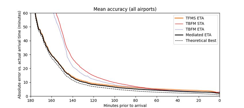
be turned on or off as needed by TMCs. Prior to freezing, the TBFM STA will typically update at a frequency about
the same as the TBFM ETA. When frozen, the TBFM STA will stop updating. The TBFM STA may be rebroadcast
periodically when frozen. It is possible for a frozen TBFM STA to become unfrozen, either because freeze horizons are
turned off, because the list of arrivals is reshuffled to address a sequencing issue, or because of a manual unfreezing
action by a TMC to re-sequence flights.

2. Mediation Rules
 Because of the differences in scope and design of TFMS and TBFM systems, there are differences in the landing
times calculated for any given flight. The ML model we developed takes only one predicted landing time as a feature for
its prediction. In this section, we describe the development of mediation rules used to decide which of the available
landing times should be used as an input for the ML model.
 While we sought to develop mediation rules that selected the physics-based prediction with the lowest errors, we
also imposed constraints on these rules. We aimed for a simple set of rules that would be easy to explain to users and to
develop and maintain. Furthermore, we decided to derive a single set of rules that applied to arrivals at all airports in the
NAS. Prediction accuracy could be improved by relaxing these constraints, but complexity of the rule set would increase.

 Before departure, use TFMS ETA
 Prior to departure, the TFMS ETA appears to be more accurate than TBFM ETA and TBFM STA. Flights that
are still on the surface should not use the TBFM ETA or TBFM STA for a predicted landing times. Figure 1 shows
accuracy of the estimates relative to the actual departure time. After departure, TBFM ETA and TBFM STA accuracy
improves and stabilizes. The figure shows mean error from a sample day of flights operated on 8/19/2019, destined
for airports with Digital-Automatic Terminal Information Service (D-ATIS) availability (76 relatively major airports).
These airports were selected to include the usefulness of checking the consistency between TBFM runway assignments
and current D-ATIS runway configuration. Because the correlation of these values did not result in an improvement in
the mediated landing time, it is not discussed further in this paper.

 Fig. 1 ETA accuracy relative to runway departure time.

 After departure, prefer TBFM STA
 TBFM systems compare the amount of expected traffic to the configured capacity of Meter Reference Elements
(fixes and arcs) within their area of responsibility. When a TBFM system expects the capacity of its resources to be
exceeded by the demand, it calculates a TBFM STA that includes the amount of time it expects the flight needs to satisfy
the constraint of the affected resources. If the TBFM system does not detect such a demand-capacity imbalance, the
TBFM STA and TBFM ETA will be equal to one another. However, because the TBFM STA and TBFM ETA are not
published in the same message, the latest available TBFM STA or TBFM ETA visible to SWIM consumers may not
precisely reflect the current expectations of the publishing TBFM system.
 When all three estimates (TBFM STA, TBFM ETA, and TFMS ETA) are available, the TBFM STA appears to be
most often closer to the actual landing time. This can be seen in Figure 2, which plots the mean accuracy for each
estimate across all available airports for the last 30 minutes of the flights. The lines show the mean absolute difference
between value available from the estimate and the actual landing time, as the flight approaches actual landing time. The

 4

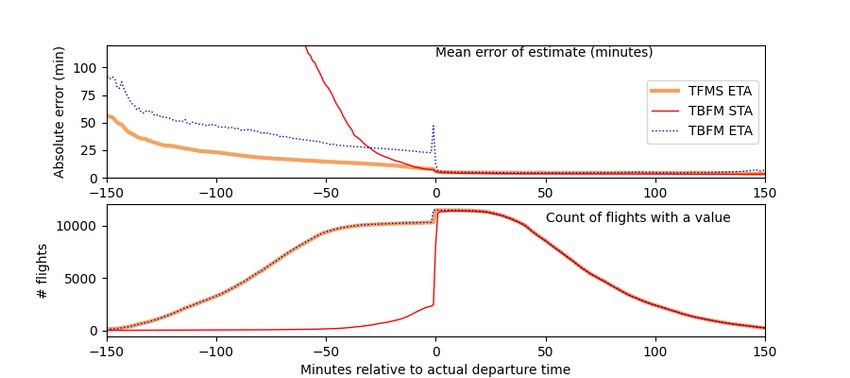
Fig. 2 Mean ETA accuracy (final 30 minutes).

dashed line shows a theoretical “best” ETA, using whichever of the three available times is closest to the actual arrival
time at each instant and for each flight.
 Typically within minutes after a flight departs, the flight starts being “tracked” by the destination TBFM system. This
is about the time the flight is picked up by the radar surveillance system, and not necessarily the time the flight took off.
 When a flight is not tracked by the TBFM facility, the TBFM ETA may not be updated consistently, which
may cause stale estimates. Ideally, our mediation rules would key off this tracked indicator. Because dif-
ferent TBFM systems may begin tracking the same flight at different times, and because the flight may be
dropped and tracked again, it can be challenging to extract this data element from the data feed. For this ef-
fort, we choose the simple approach of using the flight’s departure status as a proxy for the tracked indicator.

 Account for inconsistencies near the arrival time
 In the last few minutes of a flight, the flight passes the arrival fix, and the accuracy of the TBFM ETA and TBFM
STA can deteriorate prior to landing. Around this time, the flight is being handed off between the Air Route Traffic
Control Center (ARTCC) and a Terminal Radar Approach Control (TRACON) facilities. The en route controller
is effectively finished with the flight, and thus no longer separating the flight at the fix to which the TBFM STA is
referenced. This can be seen in the last few minutes of Figure 2, as the mean absolute error for TBFM ETA and TBFM
STA begins to increase slightly in the last few minutes to arrival, while TFMS ETA appears to improve.
 At this same time, the TFMS ETA may fall to a time in the past until it is corrected after the flight lands. The closer
to landing on the runway, the more flights had TFMS ETA values in the past. Figure 3 shows counts of arrivals as they
approach their actual landing time. The flights are split into those whose latest published TFMS ETA had a value which
was still a future time relative to the current time, and those whose latest published TFMS ETA has gotten stale to the
point where it implied the flight should have arrived already (at the bottom right of the figure).

 Fig. 3 State of TFMS ETA relative to current time.

 Given that the TBFM ETA and TBFM STA appear to lose their predictive value when the aircraft is very near its

 5

landing time, the TFMS ETA is presumed to be the more accurate estimate in these cases, regardless of the existence of
the TBFM STA. When the TFMS ETA indicates a time in the past, that time will be used at the mediated landing time.

3. Implemented mediation rules
 The mediation rules that were used are summarized in Algorithm 1. Applying these rules improved the mediated
arrival estimate (black line in Figure 4) compared to only using the TFMS ETA. However, the “theoretical best”
(dashed line), below the mediated error line, indicates there are more improvements that could be made to this estimate.
 Algorithm 1: Mediation rules for physics-based predictions
 if TFMS ETA ≤ now then // when TFMS ETA is in the past, use it
 return TFMS ETA
 else if (flight is airborne) and (TBFM STA > now) then// use TBFM STA after departure and while
 it is in the future
 return TBFM STA
 else if TFMS ETA not null then// use TFMS ETA as soon as it is available through departure
 return TFMS ETA
 else
 return null
 end

 Fig. 4 Mean ETA accuracy (final 3 hours).

B. Machine Learning for Predicting Landing Times

1. Data sources
 Not all the available data used for modeling was machine-readable after being parsed from available data feeds.
Three sets of “adaptation” data were required for the development of the ML models. Adaptation data describes
characteristics of airspace, airports, aircraft, or other relevant entities in a way that is machine-readable and can be
leveraged by ML model-training algorithms or other computer programs for which such data are relevant. Although
adaptation data can greatly empower such programs and indeed is sometimes required, it is also expensive to produce
and maintain in the sense that it requires substantial domain expertise and tedious effort to generate and update. To
reduce this labor and facilitate easy deployment at new airports, we have deliberately avoided adaptation data wherever
possible. In many cases, the information provided by adaptation data can be extracted from training data and/or it is not
required by ML models.
 The first set of adaptation data we utilized is a classification of aircraft types into classes like narrow body, wide
body, and regional jet. Aircraft types are typically stored as an encoded value in flight data. The FAA lists hundreds of
such encoded values in their Aircraft Type Designators documentation [12]. The encoded values in the flight data are
a level of abstraction from one or more individual aircraft models, and the classes are a further abstraction to group
together many of these encoded values.

 6

The second is a list of known runways at the airport for which a model is being developed. This could be learned
from the data, but an explicit specification of candidate runway names facilitates coordination between this ML model
and an upstream arrival runway prediction model. The FAA regularly publishes an updated list of airports and their
runways in its 28-day chart updates [13].
 The third is FAA National Flight Data Center (NFDC) airport runway polygons. These runway polygons represent
the area of each runway defined for each modeled airport. These polygons can be compared to surveillance data to
determine when a particular aircraft has moved onto a runway surface.
 Essentially all of the data used in the landing time prediction models come from publicly-available FAA SWIM data
feeds. This National Airspace System (NAS)-wide data was processed, synthesized, and loaded into a database by the
Fuser system developed by NASA and Mosaic ATM [14]. The FAA systems that produce data that were Fused and then
used or intended to be used for this effort are:
 • Time-Based Flow Metering (TBFM),
 • Traffic Flow Management System (TFMS), and
 • Airport Surface Detection Equipment, Model X (ASDE-X).
More particularly, we queried the Fused data to generate the following raw data for each flight bound to an arrival
airport:
 • TBFM messages,
 • TFMS surveillance data,
 • Flight characteristics such as aircraft type and carrier,
 • Actual times known when flights are airborne, such as gate departure and take off times, and
 • Airline-scheduled times such as landing times.
 Although the actual time a flight lands at its destination airport is available in FAA SWIM data, the runway on
which the flight lands is not. For this effort, we derived both of these data elements from surveillance data (ASDE-X or
TFMS) and NFDC runway adaptation data [13] to ensure consistency and reliability of these crucial data elements.
When surveillance located a flight within a runway polygon and with physics consistent with aircraft landing, it was
straightforward to determine that the flight arrived on that runway at a certain time.
 In some cases, surveillance data was not available to definitively assess the arrival runway and time. Although
this situation was relatively rare at large airports, we were able to approximate the values when necessary. We used
the airborne surveillance data from TFMS to infer which runway was used, and at what time the aircraft landed. We
accomplished this with a simple physics-based approach developed by Robert Kille [15].
 The results presented here are based only on flights for which we were able to directly assess the landing runway and
time. We omit those cases for which we had to rely on airborne surveillance and the Kille Method, which is less reliable
than the more direct assessment. Even so, predictions of landing times can be produced for flights regardless of which
approach is used after the landing event to infer the actual landing runway and time. The target for the ML models is the
actual landing time derived from surveillance data as described here, not any landing time recorded explicitly in SWIM
data.

2. Input to real-time ML model service
 The ML models developed for this effort have been carefully created to ensure they can be used in real-time with
readily-available data. Table 2 describes the 13 input data elements accepted by the initial ML model services. Only the
first three of the listed data elements are required to make a prediction, which is important for real-time scenarios in
which data is often missing. Imputation strategies are described in the table. For timestamp input data, missing values
are imputed with related timestamps. Missing categorical input like air carrier or arrival runway are encoded to binary
values (“one-hot encoded”). Each known category becomes a feature for the model and is set to 1 instead of 0 if and
only if the input takes on that category value. For example, a flight operating under the major air carrier American
Airlines (AAL) would have the feature major_carrier_AAL set to 1, but would have the feature major_carrier_DAL
(representing Delta Air Lines) set to 0. If a flight is missing the category information altogether, all of the associated
encoded feature columns are set to 0.
 Other input data are planned for inclusion in the future. These include surveillance data and expected runway
demand. The TFMS surveillance data describes the current physical state of the aircraft, rather than just knowing the
flight has departed from its origin. Demand at the flight’s intended runway is planned to be approximated using counts
of flights predicted to land on the same runway at roughly the same time as the flight in question.

 7

Table 2 Input to real-time ML model service

 Name Type Note
 timestamp timestamp time at which prediction is generated
 mediated landing time prediction timestamp selected from TBFM STA, TBFM ETA, and TFMS ETA
 first airborne surveillance timestamp timestamp from TFMS or TBFM
 actual take-off time timestamp impute with first airborne surveillance timestamp
 actual departure gate push-back time timestamp impute with actual take-off time
 airline-scheduled gate push-back time timestamp impute with actual
 airline-scheduled take-off time timestamp impute with actual
 airline-scheduled landing time timestamp impute with mediated landing time prediction
 TBFM arrival stream class string impute with one-hot encoding
 TBFM arrival meter fix string impute with one-hot encoding
 TBFM arrival runway string impute with one-hot encoding
 major air carrier string impute with one-hot encoding
 aircraft type string impute with one-hot encoding
 bold face indicates required inputs, all other input may be null

3. Features provided to ML model
 The ML model uses features to determine the appropriate predicted landing time for a flight. The features that have
been engineered and provided to initial ML models are shown in Table 3 for two sample airports. The first in this list
of features, seconds to arrival runway best time, represents the seconds to the mediated physics-based landing time
prediction, which is itself a prediction of the landing time. The mediated physics-based landing time prediction refers to
the arrival time estimates published by TFMS and TBFM through SWIM messages, described earlier. Other features
quantify the extent to which the flight is ahead of or behind the airline schedule, which previous research suggests is
predictive of actual landing times [7].
 Many of the features are categorical, which are encoded as separate binary features for each categorical option.
These categorical options can be particular to the modeled airport. For example, one of these categorical input features
is the TBFM arrival runway. The TBFM arrival runway is not available for every flight. When the TBFM system is
active, the TBFM arrival runway is produced by the TBFM system serving the flight’s destination. It is an expectation by

 Table 3 Features provided to ML models at KDFW and KJFK

 Name Encoding Number at KDFW Number at KJFK
 seconds to arrival runway best time none 1 1
 seconds arrival runway late none 1 1
 seconds departure stand late none 1 1
 seconds since departure runway actual time none 1 1
 seconds since time first tracked none 1 1
 seconds departure runway late none 1 1
 arrival stream class tbfm one-hot 41 16
 arrival meter fix tbfm one-hot 12 9
 arrival runway tbfm one-hot 14 8
 major carrier one-hot 3 3
 aircraft type one-hot 4 4
 predicted arrival runway one-hot 14 8
 total number of features 94 54

 8

that TBFM system of the runway the flight will be assigned. This expectation is based on TBFM’s own adaptation data
for the airport, and air traffic controller input regarding current and planned airport configuration. In the case of KDFW,
there are 7 physical runway surfaces. Each of these runways may be approached from either direction, making 14
possible values for an expected arrival runway. KJFK has 4 physical runway surfaces, therefore the number of possible
values is 8 for that input. Because there are different numbers of categories at different airports, the total number of
features can vary considerably from airport to airport.
 Another input to the model is the predicted arrival runway. This feature, by contrast to the TBFM arrival runway, is
modeled for each flight, even for those with no TBFM arrival runway provided in the SWIM data. This input is actually
generated from a separate ML model that predicts the arrival runway from some input features [16].
 As mentioned earlier, there are multiple TBFM systems serving the NAS. Each system has its own adaptation for its
area of responsibility. Within each TBFM system, areas are further divided into TRACONs, which are divided again
into airports. Each arrival airport may have its own set of defined metering resources (“meter fix”), and associated flows
of air traffic (“stream class”). This TBFM adaptation data is available in the TBFM-MIS SWIM feed, but is particular to
a given facility. TBFM also publishes the stream class associated with a particular flight. A flight arriving at KDFW
will be assigned a particular stream class by its destination TBFM system (ZFW, in the case of a KDFW arrival). A
flight arriving at KDFW from a different direction will typically be assigned a different stream class. A flight arriving at
KJFK will be assigned a stream class by a different TBFM system altogether (ZNY, in the case of a KJFK arrival).
These stream classes are specific to a flow of traffic, and allow the ML model to group flights by flow without the use of
origin airport or origin ARTCC as a feature.
 We intend to add more features for the ML model in the future. Other features that we intend to calculate and
provide to the model include the planned additional input mentioned in the previous sub-section (future arrival runway
counts) as well as differences between the current physical state of the aircraft and the typical physical state of flights at
the moment they land on the predicted runway.

4. Training and testing data set engineering
 We trained the ML model with a sample that consisted of the state of a flight bound to an airport at a particular
moment when it was airborne, as quantified by the model features, and the corresponding duration of time until it
actually landed (the target value to be predicted). To construct data sets of samples for model training and testing, we
first sampled the state of each flight bound to an airport every 30 seconds while it was airborne. Whereas the TFMS
ETA is typically updated every minute, TBFM STA and TBFM ETA may be updated every few seconds. Sampling the
data reduces some of the noise in the mediated physics-based landing time prediction values, and avoids bias when
certain periods have much more frequent updates than others for a given flight.
 We then further pared down the data using random sampling. We randomly kept 2% of these samples, which equates
to one sample every 25 minutes, on average. Similar random sampling of airborne times was used in previous research
on predicting landing times [6]. By down-sampling, we were able to reduce the volume of highly redundant samples in
our data sets.
 Finally, to break the data into train and test sets, we randomly selected 30% of dates in the data set to be used for
testing. All samples from flights that landed on those dates became test samples. This train-test split approach was used
to avoid redundancy across samples, where flights could be represented in both the training and testing data sets. Such
testing samples could be more highly correlated with training data samples than any future operational data would be
and therefore lead to test set performance that is not representative of the performance that would be achieved by a
deployed model.

5. ML model types
 The initial ML models have not been formulated to predict the time until the flight lands, but rather the error or
residual in the mediated physics-based landing time prediction for a flight. More precisely, let denote the actual
landing time of flight and let ˆ MPP
 ( ) be the mediated physics-based prediction (MPP) of the landing time for flight 
at time (where < ). Then the error or residual for flight at time is MPP
 ( ) = − ˆ MPP
 ( ). This error MPP
 ( )
 MPP
becomes the target for the ML models. The trained ML models produce a prediction ˆ ( ) of this error for flight at
time , which can be converted into a predicted landing time ˆ ( ) by simply adding it to ˆ MPP ( ):

 ˆ ( ) = ˆ MPP
 ( ) + ˆMPP
 ( ). (1)

 9

We set up the ML models to predict the errors in the mediated physics-based predictions of landing times for two
main reasons. First, these predictions are readily available and in many cases already very accurate. Second, learning
when and how an adequate predictor of a future event time is wrong is generally an easier ML problem than learning
to predict the future event time without initial predictions. In fact, although we found no previous research in which
ML models were trained to predict the errors of a physics-based predictor of landing times, multiple researchers have
developed a sequence of models in which one model predicts the residual of the previous model [5, 8] and indeed this
idea is fundamental to “boosting" ML models.
 ML models are trained to minimize a loss function quantifying their predictive performance on training data,
potentially with modifications to encourage model simplicity and prevent over-fitting to the training data. We have
investigated Random Forest with mean squared error (MSE) loss, and XGBoost with MSE loss and Huber loss functions
on two airports. This analysis is discussed in Section IV.B From our testing, we have found that in almost all error
metrics we track, the XGBoost model with Huber loss performs comparably or often much better than the Random
Forest model and the XGBoost model with MSE loss. Consequently, we trained XGBoost ML models with Huber loss
function for four more airports. More specifically, we trained XGBRegressor models as implemented in the scikit-learn
and XGBoost Python packages using the pseudo-Huber loss [17]. Each model’s hyperparameters were optimized using
scikit-learn’s GridSearchCV which performs an exhaustive search over specified parameter values using k-fold cross
validation.

 III. Data
 For an initial training and testing of landing time prediction models, we collected five months (April 2020 through
August 2020) of arrival data for Dallas/FortWorth International Airport (KDFW), George Bush Intercontinental
Airport (KIAH), Dallas Love Field Airport (KDAL), John F. Kennedy International Airport (KJFK), Newark Liberty
International Airport (KEWR), and Charlotte Douglas International Airport (KCLT). The training and testing data set
size for each airport is reported in Table 4.

 Table 4 Number of samples in data sets by airport

 Name KDFW KJFK KCLT KEWR KIAH KDAL
 Training 111, 005 99, 237 77, 364 58, 843 56, 537 77, 387
 Test 25, 508 18, 083 17, 238 13, 248 12, 874 14, 906

 IV. Initial Results
 Initial results show a general improvement by the XGBoost model over the mediated physics-based prediction
(MPP). Table 5 quantifies the performance of the MPP and ML model prediction (ML: XGBoost) of landing times
in the test data set for each airport. For the XGBoost results in this table, we have used the Pseudo-Huber loss, as it
resulted in superior performance. The duration of time until landing varies considerably across the training samples, so
prediction errors of the same duration can have substantially different operational implications. Therefore, we selected
two metrics that quantify the error (the difference between the actual and predicted arrival values) as a percentage of
the true duration of time (the difference between actual departure and actual arrival): mean absolute percentage error
(MAPE) and median absolute percentage error (MdAPE).
 The third metric is more aligned with operational use of the ML model. This metric is the percent of predictions
that are within 30 seconds of the true value (Pct predictions within 30s). The window may be of operational interest
because of the physical behavior of landing aircraft. Flights take time to slow down and exit the runway after touchdown,
typically around a minute in duration. During that time, additional flights are not permitted to land on the same runway
(barring special circumstances like formation flying). A prediction within this one-minute (±30 second) window around
the actual landing time can be thought of roughly as predicting the “correct” arrival runway landing “slot.”
 For almost all airports and metrics we see that the ML model prediction offers a modest to large improvement in
performance over the mediated physics-based prediction. The few exceptions are that for KJFK and KCLT, where
the mean absolute percentage error (MAPE) of the ML model predictions is considerably higher than the mediated
physics-based predictions (MPP) for those same airports. However, the ML model still achieves lower median absolute
percentage errors for these airports. This pair of results suggests that some outlier predictions with very large absolute

 10

Table 5 Summary of prediction quality in test data sets

 Metric Model KDFW KJFK KCLT KEWR KIAH KDAL
 MPP 9.7% 20.1% 18.7% 17.6% 30.9% 15.7%
 MAPE
 ML: XGBoost 9.3% 25.1% 25.0% 14.7% 32.3% 14.1%
 MPP 3.5% 4.1% 5.2% 3.4% 4.9% 3.1%
 MdAPE
 ML: XGBoost 3.0% 2.9% 4.9% 2.5% 3.2% 3.0%
 MPP 19.2% 6.4% 16.5% 14.7% 11.1% 22.4%
 Pct predictions within 30s
 ML: XGBoost 22.3% 9.8% 15.6% 18.1% 17.0% 24.2%
 bold face indicates the method with the better performing value

percentage errors exist, and are causing the higher mean absolute percentage error for the ML model predictions. These
large errors in the predictions can occur especially when the true time to landing is very short, and relatively small
landing time errors can equate to large percentage errors with respect to look-ahead time. At KJFK, neither model
manages to predict even 10% of landing times within ±30 seconds of the true value.
 The phenomenon of large outliers is likely also the root cause of the surprisingly high mean absolute percentage
errors for both methods at KIAH. The much smaller median absolute percentage errors at KIAH indicate that most
percentage errors are within 5% of zero.
 In general, the further a flight is from its destination airport, the more variability in the arrival time prediction.
Figure 5 shows the error distribution for KDFW and KJFK for the MPP and XGBoost models, respectively, by minutes
prior to actual arrival. The largest error distribution is seen at the left, at 5 hours prior to landing. As the flight
approaches its actual landing time (as assessed using surveillance data), the predictions tend to improve.
 The median error at each lookahead time prior to arrival is plotted as the solid blue line on the charts. In the case of
KDFW, we can see that the median error is closer to zero for the XGBoost model than the MPP model for all lookahead
times, however the 25th to 75th and 5th to 95th percentile range appears similar for both methods. For KJFK, the median is
closer to zero and the percentile ranges appear smaller in the XGBoost model throughout the lookahead time. However,

 MPP XGBoost

 KDFW

 KJFK

 Fig. 5 Error Distribution by Lookahead Time

 11

as the minutes prior to actual arrival approach zero, the error becomes larger in the KJFK predictions in one direction.
This means that we are starting to predict increasingly longer arrival times than the actual from approximately ten
minutes out. At approximately this time, the flight is transitioning from en route to terminal airspace. The NAS systems
most directly involved with the flight’s systems are changing, and the flight is merging with local traffic for landing.
 Outliers are visible in the data. Figure 6 shows one point for each predicted value, with the predicted time to landing
on the vertical axis, and the actual time on the horizontal axis. Both the MPP and XGBoost models are shown, for
KDFW and KJFK. The KDFW plots show a very reasonable pattern with no large outliers visible. The KJFK plots,
however, show a small number of large outliers in the lower left corner in which the actual time to landing was very
large (around 1400 minutes) and the predicted time to landing was very small (under a few minutes). This occurs in
both the MPP and XGBoost models therefore the large errors in the XGBoost model is due to the MPP data, as we are
learning from the residuals of this model.
 We assume there were some data quality issues for these outliers. Matching flight data to a particular flight is a
nontrivial task, and it is particularly troublesome when the source of flight data transitions between different automated
NAS systems, as is happening shortly before the flight arrives at its destination and during arrival. Flight matching is
further complicated by the reuse of flight data on sequential days. For example, a flight with a particular callsign can fly
between the same city pair on different days, which may account for the approximately 1440 minutes (24h) difference, if
the actual time to landing was assessed for the next day’s flight.

 MPP XGBoost

 KDFW

 KJFK

 Fig. 6 Predicted vs. Actual Time to Landing Scatterplots

 12

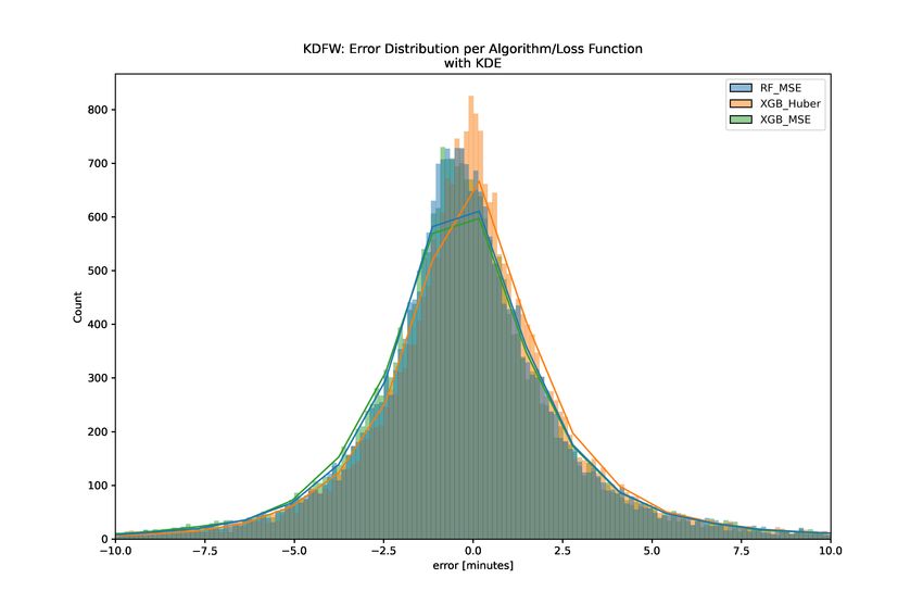
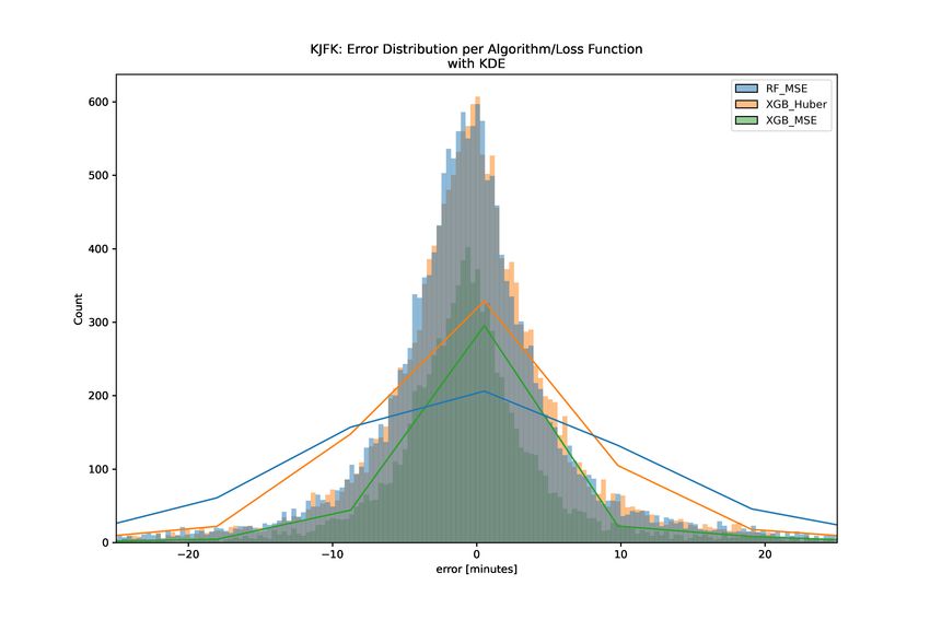
A. Evaluation of Pandemic Effects: 2019 vs 2020
 It is well known that air traffic has been greatly affected due to the pandemic. Not only did traffic counts greatly
decrease, but the way air traffic operations functioned was affected at every level. For example, air traffic control
facilities suffered staffing issues requiring the temporary closure of airspace and facilities, airline passengers required
increased screening which complicated the boarding process, and aircraft required longer times between operations to
be cleaned.
 In this section, we offer a comparison of the accuracy of the ML XGBoost model trained on 2019 data (mid-August
2019 to early December 2019) compared to the accuracy of the model trained on 2020 data (April 2020 through August
2020). The effect from year to year appears to be relatively minor regarding model accuracy. Table 6 shows the results
of this comparison for KDFW, with the error values presented for each dataset.

 Table 6 Prediction quality change in KDFW test data sets: 2019 vs 2020

 Metric 2019 2020 Change
 MAPE 15.6% 9.3% −6.3
 MdAPE 2.8% 2.9% +0.1
 Pct predictions within 30s 21.3% 22.3% +1.0
 bold face indicates the year with the better performing value

 We had hypothesized that for models in which the overall traffic patterns would affect the predicted outcome that
the performance might be worse. We did not expect, however, that the ML XGBoost model accuracy to be affected
significantly, as it is only concerned with the arrival time for a given flight. Some of the input to the model could be less
accurate (e.g. predicted arrival runway) however it was unclear how much this would impact the results.
 The comparison of the results across years does not indicate a systemic degradation of the model performance. The
results showed an improvement with the 2020 data for the Pct predictions within 30s and MAPE metrics, and relatively
small change in the MdAPE. We determined that no further exploration of the pandemic effects on the model were
needed, and no changes were made in our procedure to accommodate for pandemic effects.

B. ML Model Algorithm and Loss Function Comparison
 A potential point of contention when developing ML models is how to deal with outliers. The choice of loss function
can affect how the model learns from outliers. More specifically, mean squared error (MSE) applies much larger
importance to outliers compared to weighting them linearly as when using mean absolute error (MAE) loss function.
The Huber loss aims to offer the advantages of both the MSE and MAE loss in one piecewise function in which MAE is
used for values above a threshold and MSE for values below that threshold [18]. In the XGBoost implementation of the
Huber loss, the Pseudo-Huber loss is actually used, which ensures continuous derivatives [19].
 To investigate the loss function, we trained several algorithms for airports KDFW and KJFK. Table 7 displays the
overall accuracy results on the test set of the ML algorithms; Random Forest with MSE loss, XGBoost with MSE
loss, and XGBoost with Huber loss. The results indicate that using XGBoost with Huber loss leads to similar or more
accurate results for these metrics in almost all cases. Additionally, the MAPE is reduced for both airports with Huber
loss.
 Figure 7 shows the error distribution for the three algorithms: Random Forest, XGBoost with MSE loss, and

 Table 7 Summary of prediction quality in test data sets
 ML algorithms and loss functions

 MAPE MdAPE % within 30s
 Model KDFW KJFK KDFW KJFK KDFW KJFK
 Random Forest 12.6% 35.7% 3.1% 3.0% 19.9% 9.6%
 XGBoost MSE 12.7% 38.3% 3.2% 2.9% 19.4% 9.5%
 XGBoost Huber 9.3% 25.1% 2.9% 2.9% 22.3% 9.8%
 bold face indicates the model with the better performing value

 13

KDFW

KJFK

 Fig. 7 Histogram of Errors per Algorithm/Loss Function.

 14

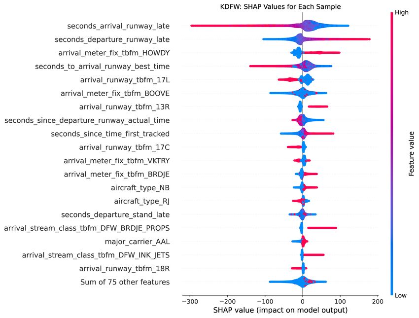
XGBoost with Huber loss on the test data. For both airports tested, KDFW and KJFK, the XGBoost with Huber
loss model (orange) displays a tighter distribution than the other two models. The XGBoost with Huber loss model
distribution appears more centered around zero minutes of error, particularly in the KDFW chart. This centering
indicates the model’s predictions are less biased.

C. Feature Importance: SHAP
 Feature importance metrics can be a valuable tool to explain the output of a predictive model. This is especially
true in the context of aviation. It is essential to operations to understand-why, for example, a certain flight is predicted
to land at a different time than expected. If a flight operator or an air traffic controller is to be able to improve their
operation in the future, they need to understand what brought about the successes or failures in previous operations.
 Conventional feature importance metrics generally look at the global importance of features to the model. With
SHAP (SHapley Additive exPlanations) [20] we can derive the local importance of features. We can also get better
information on global interpretability of feature importance. That is, we can look at a single prediction resulting from
our model, and the SHAP algorithm will help us understand how each feature in the model influenced that specific
prediction.

 Fig. 8 Aggregated Feature Importance with Collapsed Categorical Variables (KDFW XGBoost only).

 Figure 8 shows the global feature importance for the KDFW model. The features are ranked with the top as the most
influential on the model prediction. The set of encoded arrival runway features is shown to be the most influential on the
predictions for the KDFW model. In this chart, the encoded categorical variables are collapsed into a single feature, by
group. Using the SHAP method, we can see that the arrival runway expectation provided by TBFM is more important
to the model than the arrival fix provided by TBFM, for example.
 With the encoded categorical features, the influence is spread across many discrete binary features. If the features
are considered individually, the single features are ranked lower in the list. If we separated the encoded features, the
variables seconds arrival runway late and seconds departure runway late would be the top two most influential features
in the KDFW model.
 Another way to look at the relative importance of different features is to view their impact on the model output,
prediction by prediction. Figure 9 shows the impact of each feature with the positive and negative relationships of
features to the model output. Each dot is a Shapley value for a feature and data point in the training model. The x-axis
represents the impact on the model for a feature. Points that occur on the same x-axis value are jitterred so that we can
see the distribution. If that impact is positive, the feature leads to a higher prediction (a later predicted landing time). If
the impact is negative, the feature leads to a lower prediction (an earlier predicted landing time).

 15

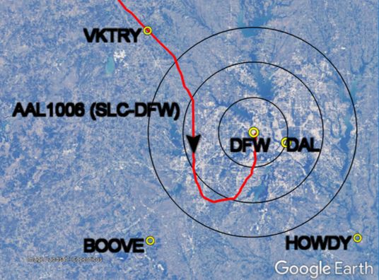
Fig. 9 Aggregated Feature Importance: SHAP Beeswarm (KDFW XGBoost only).

 The color of Figure 9 represents the high (red) or low (blue) feature values for that single data point. The seconds
arrival runway late feature had a high level of importance. It appears that seconds arrival runway late and seconds to
arrival runway best time had a tempering effect on the prediction. When these features were low (blue), the prediction
they affected still had a positive value (positive on the horizontal axis), indicating that enough of the other features
combined to cause a later prediction. With seconds departure runway late, however, in general it followed that the higher
the feature value, the higher the prediction value. The top ranked categorical feature in this list, is the feature arrival
meter fix tbfm HOWDY in third position. This feature is an indicator telling the model whether or not the given flight
was assigned to the TBFM arrival meter fix named HOWDY. HOWDY refers to a geographical point approximately 40
miles to the southeast of KDFW. HOWDY is one of many airspace waypoints that is adapted in the TBFM system for
use as a metering fix by TBFM.
 Local feature importance can be assessed for individual predictions as well. Figure 10 shows the flight path of an

Fig. 10 AAL1006 at the time of model prediction (10 NM range rings). Map data: Google, Landsat/Copernicus

 16

example flight from the dataset, callsign AAL1006 arriving at KDFW. At the moment captured in the figure, the model
was called to predict how much the MPP should be adjusted, based on the features available for the flight. At this time,
the flight was approximately 20 nautical miles West from KDFW. However, the flight still needed to adjust its path to
land in the northerly direction, which would add time to its flight beyond a simple straight-line calculation.

 Fig. 11 Single Prediction SHAP Waterfall Plot (KDFW XGBoost only).

 In this example, the model was provided the feature set for the flight. Figure 11 explains how the features were
combined to produce this single prediction. We can see that the features affected this prediction with a different relative
importance level than the aggregated set. The TBFM arrival runway for this flight was set to 35C, which increased
the value of the prediction. As a separate feature, the flight did not indicate an arrival at runway 17L (a runway in the
southerly direction). This feature contributed to further increase the value of the prediction.
 In this example, representing a single prediction for a single flight, the expected value was 32.025. This “base
value” (in gray) shows the prediction if we just took the mean value of all predictions. The model produced a value
of 85.542, after incorporating all effects of the features. This means the model predicted that an extra 85 seconds
of flying time should be added to the MPP. If the MPP was ’2020-04-12T21:55:02Z’ for this flight, which was its
TBFM STA at the moment the model was called, the prediction would have provided ’2020-04-12T21:56:27Z’ as its
improved landing time. Based on position data available on TFMData SWIM feed, this flight landed at approximately
’2020-04-12T22:00:02Z’, which indicates the flight added even more to its flight time than the model predicted.
 In the waterfall chart, we can see the amount that each feature contributes to the prediction from the mean prediction.
For example, the feature seconds departure runway late (660) contributes +19.17 to the prediction. The red coloring
means positive influence on the prediction. By contrast, seconds to arrival runway best time (558) reduced the output of
the model by 25.7. Despite seconds to arrival runway best time being the largest contributor to the shift, and shifting in
the negative direction, the output was still higher than the expected value. In this way, we can use the SHAP method to
obtain interpretable operational information on how our model’s predictions are affected by the input features.

 V. Next Steps
 As mentioned previously, we plan to extend the preliminary work described here in various ways. We intend to
incorporate additional model input data and features. We plan to develop and evaluate models for arrivals at additional
airports and with much larger data sets. Finally, we will help others evaluate how to make use of our results by providing
a much richer evaluation of the models, both in terms of the quality of their predictions and the importance of various
features in determining those predictions.
 Other extensions to this line of work are also under consideration. We may implement a hybrid mediation-ML
approach in which a classification ML model is trained to select from among the physics-based landing time predictions
using a custom loss function based on the error resulting from the selected physics-based landing time prediction.

 17

Additionally, we might evaluate another operationally-available landing time prediction that is neither ML nor physics-
based. The airline-provided arrival runway time in TFMS data (available after flight departure) may be based on
airline operational goals or expectations, which can provide additional context and information for the model. Under
certain circumstances it may provide superior predictions, or at least predictions with errors that are largely statistically
independent of those of physics-based models. The airline provided prediction values could also be used as input to ML
models.

 Acknowledgments
 The authors gratefully acknowledge funding for this work from the National Aeronautics and Space Administration
(NASA) as part of the Airspace Technology Demonstration 2 (ATD-2) project.

 References
 [1] Ging, A., Engelland, S., Capps, A., Eshow, M., Jung, Y., Sharma, S., Talebi, E., Downs, M., Freedman, C., Ngo, T., et al.,
 “Airspace Technology Demonstration 2 (ATD-2) Technology Description Document (TDD),” Tech. Rep. NASA/TM-2018-
 219767, National Aeronautics and Space Administration, 2018. URL https://ntrs.nasa.gov/citations/20180002424.

 [2] Federal Aviation Administration, “JO 7110.65Y - Air Traffic Control,” online, 2019. URL https://www.faa.gov/
 regulations_policies/orders_notices/index.cfm/go/document.information/documentID/1036234.

 [3] Fernandes, A., Wesely, D., Holtzman, B., Sweet, D., and Ghazavi, N., “Using Synchronized Trajectory Data to Improve
 Airspace Demand Predictions,” Integrated Communications Navigation and Surveillance Conference (ICNS), Herndon, VA,
 USA, 2020, pp. 3C2–1–3C2–15. https://doi.org/10.1109/ICNS50378.2020.9222909.

 [4] Glina, Y., Jordan, R. K., and Ishutkina, M. A., “A Tree-Based Ensemble Method for the Prediction and Uncertainty Quantification
 of Aircraft Landing Times,” Proceedings of American Meteorological Society 10th Conference on Artificial Intelligence
 Applications to Environmental Science, New Orleans, LA, USA, 2012.

 [5] Takács, G., “Predicting flight arrival times with a multistage model,” Proceedings of IEEE International Conference on Big
 Data (Big Data), Washington, DC, USA, 2014. https://doi.org/10.1109/BigData.2014.7004435.

 [6] Kern, C. S., de Medeiros, I. P., and Yoneyama, T., “Data-driven aircraft estimated time of arrival prediction,” Proceedings of
 Annual IEEE Systems Conference (SysCon), Vancouver, BC, Canada, 2015.

 [7] Kim, M. S., “Analysis of short-term forecasting for flight arrival time,” Journal of Air Transport Management, Vol. 52, 2016,
 pp. 35–41. https://doi.org/10.1016/j.jairtraman.2015.12.002.

 [8] Achenbach, A., and Spinler, S., “Prescriptive analytics in airline operations: Arrival time prediction and cost index optimization
 for short-haul flights,” Operations Research Perspective, Vol. 5, 2018, pp. 265–279. https://doi.org/10.1016/j.orp.2018.08.004.

 [9] Dhief, I., Wang, Z., Liang, M., Alam, S., Schultz, M., and Delahaye, D., “Predicting Aircraft Landing Time in Extended-TMA
 Using Machine Learning Methods,” Proceedings of 9th International Conference for Research in Air Transportation (ICRAT),
 Tampa, FL, USA, 2020.

[10] Ayhan, S., Costas, P., and Samet, H., “Predicting estimated time of arrival for commercial flights,” Proceedings of KDD,
 London, United Kingdom, 2018.

[11] Sridhar, B., Chatterji, G. B., and Evans, A. D., “Lessons Learned in the Application of Machine Learning Techniques to Air
 Traffic Management,” Proceedings of the AIAA AVIATION Forum, 2020.

[12] Federal Aviation Administration, “JO 7360.1E - Aircraft Type Designators,” online, 2019. URL https://www.faa.gov/regulations_
 policies/orders_notices/index.cfm/go/document.information/documentID/1036757.

[13] Federal Aviation Administration, “National Flight Data Center 28 Day NASR Subscription,” online, 2020. URL https:
 //www.faa.gov/air_traffic/flight_info/aeronav/aero_data/NASR_Subscription/.

[14] Gorman, S. M., “Fuser and Fuser in the Cloud,” Tech. Rep. ARC-E-DAA-TN72700, National Aeronautics and Space
 Administration, 2019. URL https://ntrs.nasa.gov/citations/20190030496.

[15] Kille, R., “Summary of the July 1999 Internal Departure Delay Investigation for ZDV Along with New Departure Delay Data
 From ZOB, ZID, ZFW and ZDV,” unpublished internal presentation, 2004.

 18