Interactive Graph Stream Analytics in Arkouda - MDPI
←
→
Page content transcription
If your browser does not render page correctly, please read the page content below
algorithms
Article
Interactive Graph Stream Analytics in Arkouda
Zhihui Du * , Oliver Alvarado Rodriguez, Joseph Patchett and David A. Bader *

                                          Department of Computer Science, New Jersey Institute of Technology, Newark, NJ 07102, USA;
                                          oaa9@njit.edu (O.A.R.); jtp47@njit.edu (J.P.)
                                          * Correspondence: zhihui.du@njit.edu (Z.D.); bader@njit.edu (D.A.B.)

                                          Abstract: Data from emerging applications, such as cybersecurity and social networking, can be
                                          abstracted as graphs whose edges are updated sequentially in the form of a stream. The challenging
                                          problem of interactive graph stream analytics is the quick response of the queries on terabyte
                                          and beyond graph stream data from end users. In this paper, a succinct and efficient double
                                          index data structure is designed to build the sketch of a graph stream to meet general queries. A
                                          single pass stream model, which includes general sketch building, distributed sketch based analysis
                                          algorithms and regression based approximation solution generation, is developed, and a typical graph
                                          algorithm—triangle counting—is implemented to evaluate the proposed method. Experimental
                                          results on power law and normal distribution graph streams show that our method can generate
                                          accurate results (mean relative error less than 4%) with a high performance. All our methods and code
                                          have been implemented in an open source framework, Arkouda, and are available from our GitHub
                                          repository, Bader-Research. This work provides the large and rapidly growing Python community
                                          with a powerful way to handle terabyte and beyond graph stream data using their laptops.

                                Keywords: streaming graph data; graph stream sketch; triangle counting; Arkouda framework


Citation: Du, Z.; Alvarado
Rodriguez, O.; Patchett, J.; Bader, D.
Interactive Graph Stream Analytics in     1. Introduction
Arkouda. Algorithms 2021, 14, 221.              More and more emerging applications, such as social networks, cybersecurity and
https://doi.org/10.3390/a14080221         bioinformatics, have data that often come in the form of real-time graph streams [1].
                                          Over its lifetime, the sheer volume of a stream could be petabytes, or more like network
Academic Editors: Deepak Ajwani,
                                          traffic analysis in the IPv6 network, which has 2128 nodes. These applications motivate
Sabine Storandt and Darren Strash
                                          the challenging problem of designing succinct data structures and real-time algorithms
                                          to return approximate solutions. Different stream models [2–7], which allow access to
Received: 1 April 2021
                                          the data in only one pass (or multi-pass in semi-streaming algorithms), are developed
Accepted: 12 July 2021
                                          to answer different queries using a significantly reduced sublinear space. The accuracy
Published: 21 July 2021
                                          of such models’ approximate solutions is often guaranteed by a pair of user specified
                                          parameters, e > 0 and 0 < δ < 1. This means that the (1 + e) approximation ratio can be
Publisher’s Note: MDPI stays neutral
with regard to jurisdictional claims in
                                          achieved with a probability of (1 − δ). This literature provides the theoretical foundation
published maps and institutional affil-
                                          to solve the challenging large scale stream data problem.
iations.
                                                However, ignoring the hidden constants in the theoretical space and time complexity
                                          analysis can cause unacceptable performance problems in real-world applications. When
                                          different applications, such as from social, economic and natural domains, have to handle
                                          real-time large data streams as routine work, the practical performance for real-world
                                          applications becomes an even more important and urgent requirement.
Copyright: © 2021 by the authors.
                                                At the same time, graph streams need exploratory data analysis (EDA) [8–10]. Instead
Licensee MDPI, Basel, Switzerland.
                                          of checking results, given a hypothesis, with data, EDA is primarily for seeing what the
This article is an open access article
distributed under the terms and
                                          data can tell us beyond the formal modeling or hypotheses testing task. In this way, EDA
conditions of the Creative Commons
                                          tries to maximize the value of data. Popular EDA methods and tools, which often run
Attribution (CC BY) license (https://     on laptops or common personal computers, cannot hold terabyte or even larger graph
creativecommons.org/licenses/by/          datasets, let alone produce highly efficient analysis results. Arkouda [11,12] is an EDA
4.0/).                                    framework under early development that brings together the productivity of Python with

Algorithms 2021, 14, 221. https://doi.org/10.3390/a14080221                                            https://www.mdpi.com/journal/algorithms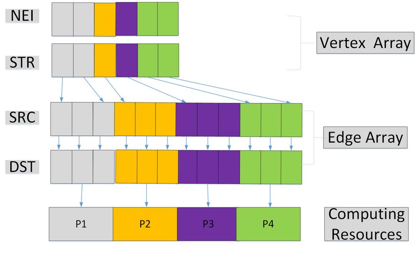
Algorithms 2021, 14, 221                                                                                        2 of 25

                           world-class high-performance computing. If a graph stream algorithm can be integrated
                           into Arkouda, it means that data scientists can take advantage of both laptop computing
                           and cloud/supercomputing to perform interactive data analysis at scale.
                                In this work, we propose a single pass stream model and develop a typical algorithm
                           for interactive graph stream analytics that can meet practical performance requirements
                           with high accuracy. Furthermore, the proposed model and algorithm will be integrated
                           into Arkouda to support the Python community to handle graph streams efficiently. The
                           major contributions of this paper are as follows:
                           1.   A succinct Double-Index (DI) data structure is designed to build the sketch of a
                                large graph stream. The DI data structure can support an edge based sparse graph
                                partition to achieve load balance and to achieve O(1) time complexity in searching
                                the incidence vertices of a given edge or the adjacency list of a given vertex.
                           2.   A single pass regression analysis stream model is developed to support general graph
                                streams analysis. Our model can map a large graph stream into a much smaller user
                                specified working space to build a general graph stream sketch. Our method can
                                improve the query quality by dividing the sketch into multiple partitions. A general
                                regression method is proposed to generate the approximate solution based on the
                                partial query results from different partitions.
                           3.   A typical graph algorithm—triangle counting [13]—is developed to evaluate the
                                efficiency of the proposed stream regression model. Experimental results using two
                                typical distributions—power law and normal distributions—show that our method
                                can achieve a high accuracy with a very low (4%) mean relative error.
                           4.   All the proposed methods have been integrated into an open-source framework,
                                Arkouda, to evaluate their practical end-to-end performance. This work can help the
                                large and popular data analytics community that exists within Python to conduct
                                interactive graph stream analytics easily and efficiently on terabytes, and beyond, of
                                graph stream data.

                           2. Related Work
                                There are two different methods for handling graph streams. One is the exact method
                           and the other is the approximate method. The exact method needs very large memory
                           to completely hold the graph stream. This is often not feasible for hardware resource
                           limited systems. The approximate method will use very limited memory (sublinear space)
                           to handle the graph streams but can only provide approximate solutions. In this section,
                           we will introduce the related approximate methods, exact methods and different triangle
                           counting algorithms.

                           2.1. Graph Stream Sketch
                                A much smaller sketch allows for many queries over the large graph stream to obtain
                           approximate results efficiently. Therefore, how to build a graph stream’s sketch is of
                           fundamental importance for graph stream analytics. There are several methods that build
                           the sketch by treating each stream element independently without keeping the relationships
                           among those elements. For example, CountMin [4] allows fundamental queries in data
                           stream summarization such as point, range, and inner product queries. It can also be
                           used to find quantiles and frequent items in a data stream. Bottom K sketch [5] places
                           both priority sampling and weighted sampling, without replacement, within a unified
                           framework. It can generate tighter bounds when the total weight is available. gSketch [6]
                           introduces the sketch partitioning technique to estimate and optimize the responses to
                           basic queries on graph streams. By exploiting both data and query workload samples,
                           gSketch can achieve better query estimation accuracy than that achieved with only the
                           data sample. In fact, we borrow the sketch partitioning idea in our implementation of the
                           Double-Index (DI) sketch. However, these existing sketches focus on ad-hoc problems
                           (they can only solve the proposed specific problems instead of general problems), so they
                           cannot support general data analytics over graph streams.
Algorithms 2021, 14, 221 3 of 25
TCM sketch [7] uses a graphical model to build the sketch of a graph stream. This
means that TCM is a general sketch that allows complicated queries. However, TCM’s focus
is setting up a general sketch theoretically, instead of optimizing the practical performance
for real-world datasets. Our Double-Index (DI) sketch is especially designed for real-world
sparse graph streams and it can achieve a high practical performance.
2.2. Complete Graph Stream Processing Method
Several dynamic graph management and analytics solutions are as follows. Aspen [14]
takes advantage of purely functional trees data structure, C-trees, to implement quick graph
updates and queries. LLAMA’s streaming graph data structure [15] is motivated by the CSR
format. However, like Aspen, LLAMA is designed for batch processing in the single-writer
multi-reader setting and does not provide graph mutation support. GraphOne [16] can run
queries on the most recent version of the graph while processing updates concurrently by
using a combination of an adjacency list and an edge list.
Systems such as LLAMA, Aspen and GraphOne focus on designing efficient dynamic
graph data structures, and their processing units do not support incremental computation.
KickStarter [17] maintains the dependency information in the form of dependency trees,
and performs an incremental trimming process that adjusts the values based on monotonic
relationships. GraphBolt [18] incrementally processes streaming graphs and minimizes
redundant computations upon graph mutations while still guaranteeing synchronous
processing semantics. DZiG [19] is a high-performance streaming graph processing system
that retains efficiency in the presence of sparse computations while still guaranteeing
BSP semantics. However, all such methods have the challenging requirement that the
memory must be large enough to hold all the streams. For very large streams, this is often
not feasible.
2.3. Triangle Counting Algorithm
Triangle counting is a key building block for important graph algorithms such as
transitivity and K-truss. There are two kinds of triangle counting algorithms, exact triangle
counting for static graphs and approximate triangle counting for graphs built from dynamic
streams [1]. Since the proposed DI sketch is a graphical model, all the static triangle
counting algorithms can also be used on the small DI sketch.
Graph Challenge https://graphchallenge.mit.edu/challenges (accessed on 20 July 2021)
is an important competition for large graph algorithms (including triangle counting). Starting
from 2017, many excellent static triangle counting algorithms have been developed. They
target three hardware platforms: shared memory, distributed memory and GPU.
The shared memory methods take advantage of some fast parallel packages, such
as Kokkos Kernels [20] or Cilk [21], to improve their performance. However, the GPU
methods [22–24] use massively parallel fine-grain hardware threads of a GPU to improve
the performance. Distributed memory triangle counting focuses on very large graphs
that cannot fit in a single node’s memory. Some heuristics [25], optimized communica-
tion libraries [26] and graph structures [27] are used to improve the performance. We
leverage the ideas in such methods to develop our Chapel-based multi-locale triangle
counting algorithm.
The basic idea of graph stream analysis is to estimate the exact query result of a
graph stream based on the sampling results. Colorful triangle counting [28] is an example.
However, it needs to know the number of triangles and the maximum number of trian-
gles of an edge to set the possibility value. This is not feasible in practical applications.
Reduction-based [29] triangle counting is a typical method, which can design a theoretical
algorithm based on user specified values (e, δ). Such a method often cannot directly be
used satisfactorily in practical applications because hidden constant values often impact the
performance. Neighborhood sampling [30] is another method for triangle counting with
significant space and time complexity improvements. Specifically, Braverman et al. [31]
discuss the difficulty of the triangle counting algorithm in a streaming model. Other sam-Algorithms 2021, 14, 221 4 of 25
pling methods, such as [32], have space usage that depends on the ratio of the number
of triangles and the number of triples, or the algorithm will require the edge stream to
meet a specific order. Jha et al. [33] apply the birthday paradox theory to sampling data to
estimate the number of triangles in a graph stream.
3. Arkouda Framework
Arkouda is an open-source framework that aims to support flexible, productive, and
high performance large scale data analytics. The basic building components of Arkouda
include three parts: the front-end (Python [34]), the back-end (Chapel [35]) and a middle,
communicative part (ZeroMQ [36]). Python is the interface for end users to utilize the
different functions from Arkouda. All large data analysis and high performance computing
(HPC) tasks are executed at the back-end (server) without users needing to know the
algorithmic implementation details. ZeroMQ is used for the data and instruction exchanges
between Python users and the Chapel back-end services.
In order to enable exploratory data analysis on large scale datasets in Python, Arkouda
divides its data into two physical sections. The first section is the metadata, which only
include attribute information and occupy very little memory space. The second section
is the raw data, which include the actual big datasets to be handled by the back-end.
However, from the view of the Python programmers, all data are directly available just
as on their local laptop device. This is why Arkouda can break the limit of local memory
capacity, while at the same time bringing traditional laptop users powerful computing
capabilities that could previously only be provided by supercomputers.
When users are exploring their data, if only the metadata section is needed, then
the operations can be completed locally and quickly. These actions are carried out just
as in previous Python data processing workflows. If the operations have to be executed
on raw data, the Python program will automatically generate an internal message and
send the message to Arkouda’s message processing pipeline for external and remote help.
Arkouda’s message processing center (ZeroMQ) is responsible for exchanging messages
between its front-end and back-end. When the Chapel back-end receives the operation
command from the front-end, it will execute the analysis task quickly on the powerful HPC
resources and large memory to handle the corresponding raw data and return the required
information back to the front-end. Through this, Arkouda can support Python users to
locally handle large scale datasets residing on powerful back-end servers without knowing
all the detailed operations at the back-end.
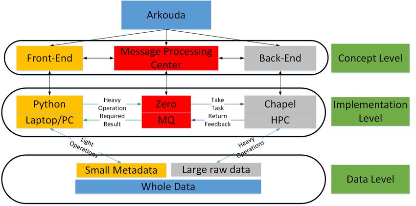
Figure 1 is a schematic diagram visualizing how Arkouda can bridge the popularity
of Python and the power of HPC together to enable EDA at scale. In this figure, from
the conceptual level view, Arkouda has three loosely coupled components. The different
components can be designed and implemented independently as long as they follow the
same information exchanging interface. Although Arkouda is implemented using Chapel,
ZeroMQ and Python, the basic concepts can be implemented with different languages and
packages. From the view of data, the data are classified into two categories, metadata and
raw data. Correspondingly, we simply refer to the operations that can be done locally and
quickly as light operations. The operations that need help from the remote server or data
center are referred to as heavy operations. Arkouda can automatically organize the data
and the corresponding operations to provide a better performance and user experience.
In this paper, we discuss the integration of our graph stream sketch, model and algo-
rithm into Arkouda to enable popular and high level Python users to conduct interactive
graph stream analytics.Algorithms 2021, 14, 221 5 of 25
Figure 1. Overview of Arkouda’s components and working mechanism.
4. Succinct Data Structure
4.1. Edge Index and Vertex Index
We propose a Double-Index (DI) data structure to support quick search from a given
edge to its incident vertices or from a given vertex to its adjacency list. The two index
arrays are called the edge index array and the vertex index array. Furthermore, our DI data
structure requires a significantly smaller memory footprint for sparse graphs.
The edge index array consists of two arrays with the same shape. One is the source
vertex array and the other is the destination vertex array. If there are a total of M edges
and N vertices, we will use the integers from 0 to M − 1 to identify different edges and the
integers from 0 to N − 1 to identify different vertices. For example, given edge e = hi, ji, we
will let SRC [e] = i and DST [e] = j, where SRC is the source vertex array and DST is the
destination vertex array; e is the edge ID number. Both SRC and DST have the same size
M. When all edges are stored in SRC and DST, we will sort them based on their combined
vertex ID value (SRC [e], DST [e]), and remap the edge ID from 0 to M − 1. Based on the
sorted edge index array, we can build the vertex index array, which also consists of two
of the same shape arrays. For example, in Figure 2, we let edge e1000 have ID 1000. If
e1000 = h50, 3i, e1001 = h50, 70i and e1002 = h50, 110i are all the edges starting from vertex
50 (a directed graph). Then we will let one vertex index array STR[50] = 1000 and another
vertex index array NEI [50] = 3. This means that, for given vertex ID 50, the edges starting
with vertex 50 are stored in the edge index array starting at position 1000 and there is a total
of 3 such edges. If there are no edges from vertex i, we will let STR[i ] = −1 and NEI [i ] = 0.
In this way, we can directly search the neighbors or adjacency list of any given vertex.
Figure 2. Double Index data structure for graph stream sketch.Algorithms 2021, 14, 221 6 of 25
Our DI data structure can also support graph weights. If each vertex has a different
weight, we use an array, V_WEI, to express the weight values. If each edge has a weight,
we use an array, E_WEI, to store the different weights.
4.2. Time and Space Complexity Analysis
For a given array A, we use A[i..j] to express the elements in A from A[i ] to A[ j]. A[i..j]
is also called an array section of A. So, for a given vertex with index i, it will have NEI [i ]
neighbors and their vertex IDs are from DST [STR[i ]] to DST [STR[i ] + NEI [i ] − 1]. This
can be expressed as an array section DST [STR[i ]..STR[i ] + NEI [i ] − 1] (here we assume
the out degree of i is not 0). For given vertex i, the adjacency list of vertex i can be easily
expressed as hi, x i, where x in DST [STR[i ]..STR[i ] + NEI [i ] − 1]. Based on the NEI and
STR vertex index arrays, we can find the neighbor vertices or the adjacency list in O(1)
time complexity. For given edge e = hi, ji, it will be easy for us to find its incident vertices
i in array SRC [e] and j in array DST [e] and also in O(1) time complexity. Regarding the
storage space, if the graph has M edges and N vertices, we will need 2M memory to store
all the edges. Compared with the dense matrix data structure, which needs N 2 memory to
store all the edges, this is much smaller. To improve the adjacency list search performance,
we use 2N memory to store the NEI and STR arrays.
Figure 2 shows M sorted edges represented by the SRC and DST arrays. Any one
of the N vertices nk can find its neighbors using NEI and STR arrays with O(1) time
complexity. For example, given edge hi, ji, if vertex j’s starting index in SRC is 1000, it has
three adjacency edges, then such edges can be found starting from index position 1000 in
arrays SRC and DST using NEI and STR arrays directly. This figure shows how the NEI
and STR arrays can help us locate neighbors and adjacency lists quickly.
For an undirected graph, an edge hi, ji means that we can also arrive at i from
j. We may use the data structures SRC, DST, STR, NEI to search the neighbors of j
in SRC. However, this search cannot be performed in O(1) time complexity. To im-
prove the search performance, we introduce another four arrays, called reversed arrays,
SRCr, DSTr, STRr, NEIr. For any edge hi, ji that has its i vertex in SRC and j vertex in
DST, we will have the corresponding reverse edge h j, i i in SRCr and DSTr, where SRCr
has exactly the same elements as in DST, and DSTr has exactly the same elements as in
SRC. SRCr and DSTr are also sorted, and NEIr and STRr are the array of the number of
neighbors and the array of the starting neighbor index just like the directed graph. So, for a
given vertex i of an undirected graph, the neighbors of vertex i will include the elements in
DST [STR[i ]..STR[i ] + NEI [i ] − 1] and the elements in DSTr [STRr [i ]..STRr [i ] + NEIr [i ] −
1]. The adjacency list of the vertex i should be hi, x i, where x in DST [STR[i ]..STR[i ]
+ NEI [i ] − 1] or hi, x i, where x in DSTr [STRr [i ]..STRr [i ] + NEIr [i ] − 1].
Given a directed graph with M edges and N vertices, our data structure will need
2( M + N ) integer (64 bits) storage or M+ 4
N
bytes. For an undirected graph, we will need
twice the storage of a directed graph. For weighted vertices and weighted edges, additional
N, M integer storage will be needed, respectively.
4.3. Edge Oriented Sparse Graph Partition
For real-world power law [37–39] graphs, the edge and vertex distributions are highly
skewed. Few vertices will have very large degrees but many vertices have very small
degrees. If we partition the graph evenly based on the vertices, it will be easy to cause
a load balancing problem because the processor that holds the vertices that have a large
number of edges will often have a very heavy load. So, we equally divide the total number
of edges into different computing nodes instead.
Figure 3 shows the basic idea of our sparse graph partition method. The edge arrays
SRC and DST will be distributed by BLOCK onto different processors to make sure most
of the processors will have the same load. When we assign an edge’s vertex entry in
index arrays NEI and STR to the same processors, this approach can increase the locality
when we search from edge to vertex or from vertex to edge. However, this requires usAlgorithms 2021, 14, 221 7 of 25
to distribute NEI and STR in an irregular way since the number of elements assigned to
different processors may be very different. In our current implementation, we just partition
NEI and STR arrays evenly as the edge arrays.
Figure 3. Edge based Sparse Graph Partition.
4.4. Comparison with CSR
The compressed sparse row (CSR) or compressed row storage (CRS) or Yale format
has been widely used to represent a sparse matrix with a much smaller space. Our double-
index data structure has some similarity with CSR. The value array of CSR is just like the
edge weight array in DI; the column array of CSR is the same as the DST array in DI; the
row array of CSR is very close to the STR in DI. CSR is a vertex oriented data structure and
it can support quick search from any vertex to its adjacency list. DI has the same function
as CSR.
The major difference between DI and CSR is that DI provides the explicit mapping
between an edge ID to its incident vertices, but CSR does not. This difference has two
effects: (1) DI can support another kind of quick search from any edge ID to its incident
vertices; however, CSR cannot, because SCR does not provide the source vertex of a given
edge ID; (2) DI can support edge oriented graph partition (see Section 4.3) based on the
explicit edge index arrays to achieve load balance; however, CSR cannot.
Another difference is that in DI we use an array NEI to explicitly represent the number
of neighbors of a given vertex to remove the ambiguous meaning of the row index array
in CSR. NEI [v] can be replaced by STR[v + 1] − STR[v] if we extend one element in the
STR array and use the multiple meanings of the row index array in CSR. In our DI data
structure, the meaning of STR[v] is not ambiguous. It is the starting position of vertex v in
the edge index array or STR[v] = −1 if v has no edge. However, in CSR, if v has no edges,
the value of STR[v] is not −1 and it is the starting position of the next non zero element
after v or the total number of non zero elements. So, for any case in which we need to
make sure STR[v] is really the starting position of v, we must execute an additional check
because the value of STR[v] itself cannot provide such information. When we use the DI
data structure to express a much smaller graph sketch, the number of the total vertices N is
much smaller than before. So, in DI we use an additional N size array NEI (much smaller
than the original graph) to ensure the parallel operations on STR have clear semantics and
are easy to understand.
5. Single Pass Regression Analysis Stream Model
Our stream model has the following features: (1) Only one pass is needed to build the
graph sketch; (2) A parameter, the Shrinking Factor, is introduced to allow users to directly
control the size of a sketch. So, the users’ requirement can be used to build a sketch withAlgorithms 2021, 14, 221 8 of 25
much less space; (3) The graph stream sketch is divided into three different partitions (we
also refer to the three independent small graphs as sub-sketches) and this method can help
us to avoid global heterogeneity and skewness but take advantage of the local similarity;
(4) Our sketch is expressed as a graph so the exact graph analysis method on a complete
graph can also be used on our different sub-sketches; (5) A general multivariate linear
regression model is used to generate the approximate solution based on the results from
different sub-sketches. The regression method can be employed to support general graph
analysis methods.
The framework of our stream model includes three parts: (1) Mapping a graph stream
into a much smaller graph sketch in one pass. The sketch can have multiple independent
partitions or sub-sketches; (2) Developing an exact algorithm on different sub-sketches to
generate partial solutions; (3) Developing a regression model to generate an approximate
solution based on different partial solutions.
5.1. Building the Sketch as a Multi-Partition Graph
5.1.1. Sliding Window Stream
We first describe our method when the stream comes from a sliding window, which
means that only the last M edges falling into the given time window will be considered.
We define the shrinking factor SF (a positive integer) to constrain the space allocation
of a stream sketch. This means that the size of the edges and vertices of the graph sketch will
1
be SF of the original graph. The existing research on sketch building [7] shows that multiple
pairwise independent hash function [4] methods can often generate better estimation results
because they can reduce the probability of hash collisions. In our solution, we sample at
different parts of the given sliding window instead of the complete stream and then map
the sampled edges into multiple (here three) independent partitions to completely avoid
collisions. We name the three partitions Head, Mid, and Tail partitions or sub-sketches,
1
respectively. Each partition will be assigned with 3SF space of the original graph.
Since we divide the sketch into three independent partitions, we select a very simple
hash function. For a given sliding window, we let the total number of edges and vertices
M
in this window be M and N. Then, the size of each partition will have Partition M = 3SF
N
edges and Partition N = 3SF vertices. For any edge e = hi, ji from the original graph, we
will map the edge ID e to mod(e, Partition M ). At the same time, its two vertices i and j
will be mapped to mod(i, Partition N ) and mod( j, Partition N ). If e < M 3 , then we will map
e = hi, ji to the Head partition. If e ≥ 2M 3 , we will map e = h i, j i to the Tail partition.
Otherwise, we will map e = hi, ji to the Mid partition.
Figure 4 is an example that shows how we map, completely, 3,000,000 edges in a given
sliding window into a sketch with three partitions. The edges from 1,000,000 to 1999,999
are mapped to the Head partition p0 that has 1000 edges. The edges from 2,000,000 to
2,999,999 are mapped to the Mid partition p1 and the edges from 3,000,000 to 3,999,999 are
mapped to the Tail partition p2. Each partition is expressed as a graph.
Figure 4. Mapping a graph stream into a multi-partition sketch.Algorithms 2021, 14, 221 9 of 25
After the three smaller partitions are built, we sort the edges and create the DI data
structure to store the partition graphs.
We map different parts of a stream into corresponding sub-sketches and this is very
different from the existing sketch building methods. They map the same stream into differ-
ent sketches with independent pairwise hash functions so each sketch is an independent
summarization of the stream. However, in our method, one sub-sketch can only stand for a
part of the stream and we use different sub-sketches to capture the different local features
in a stream. Our regression model (see Section 5.3) will be responsible for generating the
final approximate solution.
More partitions will help to capture more local features of a stream. However, we
aim for a regression model that is as simple as possible. Too many partitions will make
our regression model have more variables and become complicated. We select three as
the default number of partitions because this can achieve sufficient accuracy based on our
experimental results. Of course, for some special cases, we may choose more partitions but
use the same proposed framework.
5.1.2. Insert-Only and Insert-Delete Streams
For the sliding window stream, we only need to care about the edges in the given
window. However, for insert-only and insert-delete streams, we need to consider the edges
that will come in the future. Here, we will describe the sketch updating mechanism in our
stream model.
For the insert-delete stream, we will introduce a new weight array in the sketch. If the
total number of edges that can be held in one partition is Partition M , then we will introduce
a weight array E_WEI with size Partition M to store the latest updated information of each
edge. The initial value of E_WEI will be zero. If a new insert edge is mapped to e, then
we will let E_WEI [e] = E_WEI [e] + 1. If a deleted edge is mapped to e, then we will let
E_WEI [e] = E_WEI [e] − 1. So, for any edge in the partition, if E_WEI [e] = 0, it means
that the edge has been deleted so we can safely remove this edge from our sketch. If
E_WEI [e] > 1, it means that there are multiple edges in the stream that have been mapped
to this edge. For the insert-only stream, it is similar to the insert-delete stream but we never
reduce the value of E_WEI.
To improve the sketch update performance, we will use the bulk updating mechanism
for the two streams. If B new edges have arrived (they can be insert edges or delete edges),
we will divide B into three parts and map them into the three different partitions just as in
the method used in the sliding window stream. After the new edges are updated, we need
to resort the edges and update the DI data structure to express the updated sub-sketches.
5.2. Edge–Vertex Iterator Based Triangle Counting Algorithm
We can directly employ existing exact graph algorithms in our sketch because the
sketch is also expressed as a graph. Here, we will use a typical graph analysis algorithm—
triangle counting—to show how we can develop optimized exact algorithms based on our
DI data structure.
To improve the performance of a distributed triangle counting algorithm, two impor-
tant problems are maintaining load balancing and avoiding remote access or communica-
tion as much as possible.
In Chapel, the locale type refers to a unit of the machine resources on which the
program is running. Locales have the capability to store variables and to run Chapel tasks.
In practice, for a standard distributed memory architecture, a single multicore/SMP node
is typically considered a locale. Shared memory architectures are typically considered
a single locale. In this work, we will develop a multiple-locale exact triangle counting
algorithm for distributed memory clusters.
For power law graphs, a small number of vertices may have a high degree. So, if
we divide the data based on number of vertices, it is easy to cause an unbalanced load.
Our method divides the data based on the number of edges. At the same time, our DIAlgorithms 2021, 14, 221 10 of 25
data structure will keep the edges connected with the same vertex together. So, the edge
partition method will result in good load balancing and data access locality.
However, if each locale directly employs the existing edge iterator [13] on its edges,
the reverse edges of the undirected graphs are often not in the same locale. This will
cause a new load balancing problem. So, we will first generate the vertices based on the
edges distributed to different locales. Then, each locale will employ the vertex iterator to
calculate the number of triangles. The combined edge–vertex iterator method is the major
innovation for our triangle counting method on distributed systems.
When we employ the high level parallel language Chapel to design the parallel exact
triangle counting algorithm, there are two additional advantages: (1) Our DI data structure
can work together with the coforall or forall parallel construct of Chapel to exploit the
parallelism; (2) We can take advantage of the high level module Set provided by Chapel to
implement the parallel set operation easily and efficiently.
At a high level, our proposed algorithm takes advantage of the multi-locale feature
of Chapel to handle very large graphs in distributed memory. The distributed data are
processed at their locales or their local memory. Furthermore, each shared memory compute
node can also process their own data in parallel. The following steps are needed to
implement the multi-locale exact triangle counting algorithm: (1) The DI graph data should
be distributed evenly onto the distributed memory to balance the load; (2) Each distributed
node only counts the triangle including the vertices assigned to the current node; (3) All
the triangles calculated by different nodes should be summed together to obtain the exact
number of triangles.
Our multi-locale exact triangle counting algorithm is described in Algorithm 1. For
a given graph sketch partition Gsk = h Esk , Vsk i, we will use an array subTriSum to keep
each locale’s result (line 2). Here in line 3, we use coforall instead of forall to allow each loc
in Locales to execute the following code in parallel so we can fully exploit the distributed
computing resources. The code between line 3 and line 17 will be executed in parallel on
each locale. Each locale will use a local variable triCount to store the number of triangles
(line 5). Line 6 and line 7 are important for implementing load balancing. Assume edges
from estart to eend are assigned to the current locale, we can obtain the corresponding vertex
ID StartVer = SRC [estart ] and EndVer = SRC [eend ] as the vertices interval that the current
locale will handle. Since different locales may have different edges with the same starting
vertex, the interval [StartVer..EndVer ] of different locales may overlap. At the same time,
some starting vertex in the SRCr index array may not appear in SRC, so we should also
make sure there is no “hole” in the complete interval [0..|Vsk | − 1]. In line 7, we will make
sure all the intervals will cover all the vertices without overlapping.
Our method includes the following steps: (1) If the current locale’s StartVer is the
same as the previous locale’s EndVer, this means that one vertex’s edges have been parti-
tioned into two different locales. We will set StartVer = StartVer + 1 to avoid two locales
executing the counting on the same vertex; (2) If the current locale’s StartVer is different
from the previous locale’s EndVer, and the difference is larger than 1, this means that there
is a “hole” between the last locale’s vertices and the current locale’s vertices. So we will let
the current locale’s StartVer = last locale’s EndVer + 1; (3) If the current locale is the last
locale, we will let its EndVer = the last vertex ID. If the current locale is the first locale, we
will let StartVer = 0.
From line 8 to line 14 we will count all the triangles starting from the vertices assigned
to the current locale in parallel. In line 9 we will generate all the adjacent vertices u adj of
the current vertex u and its vertex ID is larger than u. From line 10 to line 12, for any vertex
v ∈ u adj , we will generate all the adjacent vertices v adj of current vertex v and its vertex ID
is larger than v. So the number of vertices in u adj ∩ v adj is the number of triangles having
edge hu, vi. Since we only calculate the triangles whose vertices meet u < v < w, we will
not count the duplicate triangles. In this way, we can avoid the unnecessary calculation. In
line 15, each locale will assign its total number of triangles to the corresponding positionAlgorithms 2021, 14, 221 11 of 25
of array subTrisum. At the end in line 18, when we sum all the number of triangles of
different locales, we will obtain the total number of triangles.
Algorithm 1: Edge–vertex Iterator triangle counting algorithm
1 TC ( Gsk = h Esk , Vsk i)
/* Gsk is the given graph sketch partition,Esk , Vsk are edge and
vertex sets. */
2 var subTriSum=0: [0..numLocales-1] int;//store each locale’s number of triangles
3 coforall (loc in Locales) do
4 if (current loc is my locale) then
5 var triCount=0:int;//initialize number of local triangles
6 Assign StartVer and EndVer based on edge index array
7 Adjust StartVer and EndVer to cover all vertices and avoid overlapping
8 forall (u in StartVer..EndVer with (+ reduce triCount)) do
9 u adj = { x |hu, x i ∈ Esk ∧ ( x > u)} //build the u adjacency vertex set in
parallel
10 forall v ∈ u adj do
11 v adj = { x |hv, x i ∈ Esk ∧ ( x > v)} //build the v adjacency vertex set
in parallel
12 end
13 TriCount+ = |u adj ∩ v adj |;
14 end
15 subTriSum[here.id] = triCount;
16 end
17 end
18 return sum ( subTriSum )
5.3. Real-World Graph Distribution Based Regression Model
Instead of developing different specific methods for different graph analysis problems,
we propose a general regression method to generate the approximate solution based on the
results of different sub-sketches.
One essential objective of a stream model is generating an accurate estimation based
on the query results from its sketch. The basic idea of our method is to exploit the real-
world graph distribution information to build an accurate regression model. Then we can
use the regression model to generate approximate solutions for different queries.
Specifically, for the triangle counting problem, when we know the exact number of
triangles in each sub-sketch (see Table 1), the key problem is how we can estimate the total
number of triangles.
To achieve user-required accuracy for different real-world applications, our method
exploits the features of real-world graph distributions. Many sparse networks—social
networks in particular—have an important property; their degree distribution follows
the power law distribution. Normal distributions are often used in the natural and social
sciences to represent real-valued random variables whose distributions are not known. So,
we develop two regression models for the two different graph degree distributions.
We let EH , E M , ET be the exact number of triangles in the Head, Mid and Tail sub-
sketches. The exact triangle counting algorithm is given in Section 5.2.
For normal degree distribution graphs, we assume that the total number of trian-
gles has a linear relationship with the number of triangles in each sub-sketch. We take
EH , E M , ET as three randomly sampled results of the original stream graph to build our
multivariate linear regression model. TCNormal is the estimated number of triangles and
the regression model is given in Equation (1).
TCNormal = a × EH + b × E M + c × ET . (1)Algorithms 2021, 14, 221 12 of 25
Table 1. Sketch Triangle Number.
Graph Name Shrinking Factor Head Mid Tail Exact
delaunay_n10 4 98 138 150 2047
delaunay_n10 8 63 72 80 2046
delaunay_n10 16 35 41 41 2044
delaunay_n10 32 20 12 16 2043
delaunay_n10 64 3 3 10 2042
delaunay_n11 4 195 302 294 4104
delaunay_n11 8 95 151 144 4103
delaunay_n11 16 62 71 63 4101
delaunay_n11 32 26 32 29 4100
delaunay_n11 64 12 24 14 4009
delaunay_n12 4 258 607 575 8215
delaunay_n12 8 163 306 293 8214
delaunay_n12 16 90 139 147 8212
delaunay_n12 32 52 78 76 8211
delaunay_n12 64 51 42 32 8210
delaunay_n13 4 646 1160 1197 16,442
delaunay_n13 8 335 598 588 16,441
delaunay_n13 16 187 297 304 16,439
delaunay_n13 32 108 144 153 16,438
delaunay_n13 64 68 62 81 16,437
delaunay_n14 4 1099 2356 2299 32,921
delaunay_n14 8 507 1205 1184 32,920
delaunay_n14 16 269 568 579 32,918
delaunay_n14 32 135 294 303 32,917
delaunay_n14 64 93 144 137 32,916
delaunay_n15 4 2085 4571 4585 65,872
delaunay_n15 8 943 2335 2320 65,871
delaunay_n15 16 486 1140 1159 65,869
delaunay_n15 32 265 568 580 65,868
delaunay_n15 64 137 282 299 65,867
delaunay_n16 4 4168 9648 9510 131,842
delaunay_n16 8 2170 4666 4601 131,841
delaunay_n16 16 1063 2387 2348 131,839
delaunay_n16 32 569 1174 1169 131,838
delaunay_n16 64 326 576 580 131,837
delaunay_n17 4 8154 18,873 18,938 263,620
delaunay_n17 8 4012 9543 9501 263,619
delaunay_n17 16 2132 4595 4773 263,617Algorithms 2021, 14, 221 13 of 25
Table 1. Cont.
Graph Name Shrinking Factor Head Mid Tail Exact
delaunay_n17 32 1042 2288 2347 263,616
delaunay_n17 64 534 1156 1180 263,615
delaunay_n18 4 16,904 37,774 38,061 527,234
delaunay_n18 8 8155 19,005 19,107 527,233
delaunay_n18 16 4176 9454 9562 527,231
delaunay_n18 32 2097 4674 4686 527,230
delaunay_n18 64 1004 2369 2348 527,229
amazon 4 4944 6383 18,381 667,259
amazon 8 1427 1752 7351 667,258
amazon 16 621 617 3614 667,256
amazon 32 331 290 2250 667,255
amazon 64 177 153 1546 667,254
dblp 4 20,269 41,390 168,996 2,225,882
dblp 8 6876 17,043 67,782 2,225,881
dblp 16 2684 4846 20,310 2,225,879
dblp 32 1097 2726 11,456 2,225,878
dblp 64 545 2325 2678 2,225,877
ca-HepTh.txt 4 1267 1072 3853 28,677
ca-HepTh.txt 8 642 591 1741 28,676
ca-HepTh.txt 16 456 390 480 28,674
ca-HepTh.txt 32 391 267 219 28,673
ca-HepTh.txt 64 260 217 157 28,672
ca-CondMat.txt 4 7960 10,280 12,051 174,578
ca-CondMat.txt 8 4264 4970 5543 174,577
ca-CondMat.txt 16 2862 2847 2655 174,575
ca-CondMat.txt 32 1888 1693 1403 174,574
ca-CondMat.txt 64 1179 1292 845 174,573
ca-AstroPh.txt 4 75,594 78,234 78,855 1,374,119
ca-AstroPh.txt 8 41,331 47,387 40,395 1,374,118
ca-AstroPh.txt 16 24,828 28,244 20,468 1,374,116
ca-AstroPh.txt 32 14,984 16,692 11,128 1,374,115
ca-AstroPh.txt 64 6450 6507 6322 1,374,114
email-Enron.txt 4 70,077 28,783 25,933 727,044
email-Enron.txt 8 22,331 13,593 15,197 727,043
email-Enron.txt 16 11,640 8381 5002 727,041
email-Enron.txt 32 6681 5212 2392 727,040
email-Enron.txt 64 3561 2912 1056 727,039Algorithms 2021, 14, 221 14 of 25
Table 1. Cont.
Graph Name Shrinking Factor Head Mid Tail Exact
ca-GrQc.txt 4 1193 3374 5300 48,265
ca-GrQc.txt 8 671 2131 1096 48,264
ca-GrQc.txt 16 346 880 733 48,262
ca-GrQc.txt 32 276 694 385 48,261
ca-GrQc.txt 64 64 221 150 48,260
ca-HepPh.txt 4 118,540 74,598 187,003 3,345,241
ca-HepPh.txt 8 44,937 33,404 64,281 3,345,240
ca-HepPh.txt 16 16,775 16,426 35,817 3,345,238
ca-HepPh.txt 32 3708 6643 8724 3,345,237
ca-HepPh.txt 64 705 3707 2899 3,345,236
loc-brightKite_edges.txt 4 12,232 4435 2489 301,812
loc-brightKite_edges.txt 8 5266 3217 1652 301,811
loc-brightKite_edges.txt 16 2579 1673 927 301,809
loc-brightKite_edges.txt 32 1061 1335 380 301,808
loc-brightKite_edges.txt 64 552 856 280 301,807
For power law graphs, the sampling results of EH , E M , ET can be significantly different
because of the skewness in degree distribution. A power law distribution has the property
that its log–log plot is a straight line. So we assume the logarithmic value of the total number
of triangles in a stream graph should have a linear relationship with the logarithmic values
of the exact number of triangles in different degree sub-sketches. Then we have two ways
to build the regression model. One is unordered and the other is ordered. The unordered
model can be expressed as in Equation (2). In this model, the relative order information of
sampling results cannot be captured.
TC powerlaw,log = a × EH,log + b × E M,log + c × ET,log , (2)
where TC powerlaw,log = log( TC powerlaw ) is the logarithmic value of the estimated value
TC powerlaw ; EH,log = log( EH ), E M,log = log( E M ), and ET,log = log( ET ); log( EH ), log( E M ),
and log( ET ) are the logarithmic values of EH , E M , and ET , respectively.
Then, we refine the regression model for power law distribution as follows. We get
Emin , Emedian and Emax by sorting EH , E M , and ET . They mean the minimum, median and
maximum sampling values of the number of triangles. They will be used to stand for
the sampling results of a power law distribution at the right (low possibility), middle (a
little bit high possibility) and left part (very high possibility). We let Emin,log = log( Emin ),
Emedian,log = log( Emedian ), and Emax,log = log( Emax ). Our ordered multivariate linear
regression model for power law graphs is given in Equation (3).
TC powerlaw,log = a × Emin,log + b × Emedian,log + c × Emax,log . (3)
The accuracy of our multivariate linear regression model is given in in Section 7.3.1
and we can see that the ordered regression model is better than the unordered regression
model. Both of our normal and ordered power law regression models achieve a very
high accuracy.Algorithms 2021, 14, 221 15 of 25
6. Integration with Arkouda
Based on the current Arkouda framework, the communication mechanism can be
directly reused between Python and Chapel. To support large graph analysis in Arkouda,
the major work is implementing the graph data structure and the corresponding analysis
functions in both Python and the Chapel package. In this section, we will introduce how we
define the graph classes to implement our DI data structure and develop a corresponding
Python benchmark to drive the triangle counting method.
6.1. Graph Classes Definition in Python and Chapel
Our DI data structure can also support graph weight. If each vertex has a different
weight, we use an array V_WEI to express the weight values. If each edge has a weight,
we use an array E_WEI to stand for different weights. Based on our DI data structure,
four class directed graph (GraphD), directed and weighted graph (GraphDW), undirected
graph (GraphUD) and undirected and weighted graph (GraphUDW) are defined in Python.
Four corresponding classes—SegGraphD, SegGrapDW, SegGraphUD, SegGraphUDW—
are also defined in Chapel to present different kinds of graphs. In our class definition,
directed graph is the base class. Then, undirected graph and directed and weighted
graph are the two child classes. Finally, undirected and weighted graph will inherit from
undirected graph.
All the graph classes, including their major attributes, are given in Table 2. The
left columns are the Python classes and their descriptions. The right columns are the
corresponding Chapel classes and their descriptions. Based on the graph class definition,
we can develop different graph algorithms.
6.2. Triangle Counting Benchmark
To compare the performance of the exact method and our approximate method, we
implement two triangle counting related functions. For the exact method, we implement
the “graph_file_read” and “graph_triangle” Python functions to read a complete graph
file and call our triangle counting kernel algorithm (Algorithm 1) to calculate the number
of triangles.
For our approximate method, we implement the “stream_file_read” function to simu-
late the stream by reading a graph file’s edges one by one. The graph sketch introduced
in Section 5.1 will be built automatically when we read the edges. Currently, we only
implement the sliding window streaming’s sketch building. Automatically building the
insert-only and insert-delete streaming will be future work after we evaluate our data
structure and sketch with a larger collection of graph algorithms.
After the sketch of a sliding window stream is built in the memory, we will call on the
“stream_tri_cnt” function to first calculate the exact number of triangles in each sub-sketch
(it will also call on our kernel triangle counting Algorithm 1) and then use the regression
model to estimate the total number of triangles in the given stream.
For the power law distribution regression model, in the benchmark we also implement
single variable regression models using the maximum, minimum and median results of
the three sub-sketches respectively. Our testing results show that the proposed regression
method in Section 5.3 can achieve a better accuracy.Algorithms 2021, 14, 221 16 of 25
Table 2. Double-Index Sparse Graph Class Definition in Python and Chapel.
Python Chapel
Class Attribute and Description Class Attribute and Description
n_vertices : number of vertices n_vertices : number of vertices
n_edges: number of edges n_edges: number of edges
directed: directed graph or not directed: directed graph or not
weighted: weighted graph or not weighted: weighted graph or not
GraphD SegGraphD
src : the source of every edge in the graph srcName/src : the name and data of source array
dst : the destination of every edge in the graph dstName/dst: the name and data instance of the destination array
start_i : starting index of all the vertices in src startName/start_i: the name and data instance of the starting index array
neighbor: number of neighbors all the vertices neighborName/neighbor: the name and data instance of the neighbor array
v_weight : weight of vertex v_weightName/v_weight : name and data instance of the vertex weight array
GraphDW(GraphD) SegGraphDW:SegGraphD
e_weight: weight of edge e_weightName/e_weight:name and data instance of the edge array
srcR: the source of every reverse edge in the graph srcNameR/srcR : name and data instance of the reverse source array
dstR : the destination of every reverse edge in the graph dstNameR/dstR: the name and data instance of the reverse destination array
GraphUD(GraphD) SegGraphUD:SegGraphD
start_iR : starting index of all the vertices in reverse src startNameR/starti R: the name and data of the reverse starting index array
neighborR: number of neighbors all the vertices in srcR neighborNameR: the name and data of the reverse neighbor array
v_weight : weight of vertex v_weightName/v_weight : the name and data of the vertex weight array
GraphUDW(GraphUD) SegGraphUDW:SegGraphUD
e_weight: weight of edge e_weightName:the name and data of the edge arrayAlgorithms 2021, 14, 221 17 of 25
7. Experiments
7.1. Experimental Setup
Testing of the methods was conducted in an environment composed of a 32 node
cluster with an FDR Infiniband between the nodes in the cluster. Infiniband connections
between nodes is commonly found in high performance computers. Every node is made
up of 512 GB of RAM and two 10-core Intel Xeon E5-2650 v3 @ 2.30 GHz processors with
20 cores total. Due to Arkouda being designed primarily for data analysis in an HPC
setting, an architecture setup that aptly fits an HPC scenario was chosen for testing.
7.2. Datasets Description and Analysis
We will use graph files and read the edges line by line to simulate the sliding window
of a graph stream. The graphs selected for testing were chosen from various publicly
available datasets for the benchmarking of graph methods. These include datasets from the
10th DIMACS Implementation Challenge [40], as well as some real-life graph datasets from
the Stanford Network Analysis Project (SNAP) http://snap.stanford.edu/data/ (accessed
on 20 July 2021). Pertinent information about these datasets for the triangle counting
method are displayed in Table 3.
Table 3. Graph benchmarks utilized for the triangle counting algorithm.
Degree Distribution Graph Name Edges Vertices Mean Standard Deviation
delaunay_n10 3056 1024 5.96875 3.10021
delaunay_n11 6127 2048 5.98340 3.76799
delaunay_n12 12,264 4096 5.98828 3.49865
delaunay_n13 24,547 8192 5.99292 3.25055
Normal
delaunay_n14 49,122 16,384 5.99634 3.30372
delaunay_n15 98,274 32,768 5.99817 3.37514
delaunay_n16 196,575 65,536 5.99899 3.35309
delaunay_n17 393,176 131,072 5.99938 3.26819
delaunay_n18 786,396 262,144 5.99972 3.2349
Degree Distribution Graph Name Edges Vertices a k
amazon 925,872 334,863 1,920,877 2.81
dblp 1,049,866 317,080 3,299,616.65 2.71
youtube 2,987,624 1,134,890 701,179.83 1.58
lj 34,681,189 3,997,962 50,942,065.49 2.40
orkut 117,185,083 3,072,441 40,351,890.91 2.12
ca-HepTh 51,971 9877 23,538.9 2.29
power law ca-CondMat 186,936 23,133 68,923.6 2.23
ca-AstroPh 396,160 18,772 46,698.3 1.84
email-Enron 367,662 36,692 10,150.2 1.54
ca-GrQc 28,980 5242 6610.35 2.04
ca-HepPh 237,010 12,008 4601.72 1.44
loc-brightkite_edges 214,078 58,228 44,973.1 1.88
Based on the graphs’ degree distribution, we divided them into two classes, normal
distribution and power law distribution. Prior research has shown that some real-world
graphs follow power law distributions. Normal distributions are also found ubiquitouslyAlgorithms 2021, 14, 221 18 of 25
in the natural and social sciences to represent real-valued random variables whose distri-
butions are not known. For normal distributions, their typical parameters, the mean and
standard deviation fitted from the given graphs, are listed in Table 3 too. Figure 5 shows
the comparison between the fitting results and the original graph data. We can see that the
fitting results can match with the original data very well. In other words, the Delaunay
graphs follow the normal distribution.
For graphs that follow the power law distribution y( x ) = a × x −k , we also present
their fitting parameters a and k in Table 3. Figure 6 provides some examples of these graphs.
We can see that, in general, their signatures are close to power laws. However, we can also
see that some data do not fit a power law distribution very well.
(a) Delaunay_n10 (b) Delaunay_n14 (c) Delaunay_n18
Figure 5. Normal distribution graphs.
(a) Amazon (b) dblp (c) email-Enron
Figure 6. Power law distribution graphs.
7.3. Experimental Results
7.3.1. Accuracy
In order to evaluate the accuracy of our method, we conducted experiments on nine
normal distribution and 12 power law distribution benchmark graphs with shrink factors
4, 8, 16, 32, and 64. In total, we have 105 test cases. For each test, we will have three triangle
numbers for the Head, Mid and Tail sketch partitions. We will use the exact number of
triangles in the three sub-sketches to provide the approximate number of triangles in the
given graph stream. The testing results are given in Table 1.
For the normal distribution, based on our regression model expressed as Equation (1),
we can get the parameters and express the multivariate linear regression equation as:
TCNormal = 0.7264 × EH + 1.4157 × E M + 1.7529 × ET .
When we compute the absolute value of all the percent error, the mean error is 4%,
the max error is 25% and the R-squared value is 1, and this means that the sketch results
are absolutely related to the final number of triangles.Algorithms 2021, 14, 221 19 of 25
We also evaluated our regression model to see how the accuracy changes with the
shrinking factor. For a normal distribution, we built five regression models by selecting the
shrinking factors as 4, 8, 16, 32, and 64, respectively. The result is shown in Figure 7. We
can see that both the mean and max error will increase when we doubly increase the value
of the shrinking factor step by step. However, the mean increases very slowly. The mean
error changes from 1% to 5.97%. The max error will increase from 3.36% to 26.87%. This
result shows that our regression model for normal distribution graphs is stable and very
accurate. When the graph size shrinks to half of its previous size, there is a very small effect
on the accuracy when the number of triangles is not less than some threshold value. This is
important because we can use much smaller sketches to achieve very accurate results.
For the power law distribution, based on our ordered regression model in Equation (3)
which is refined from the unordered regression model, the log value multivariate linear
regression equation can be expressed as:
TC powerlaw,log = −0.4464 × Emin,log + 0.1181 × Emedian,log + 1.4236 × Emax,log .
The mean error is 3.2%. The max value is 7.2%. The R-squared value is 0.91. This
means that the model can describe the data very well. If we use the unordered regression
model, Equation (2), the mean error is 4.5%. The max value is 12.5%. R-squared is 0.81. All
the results are worse than the results of the ordered regression model in Equation (3).
(a) Normal Distribution (b) Power Law Distribution
Figure 7. How accuracy changes with shrinking factor for normal and power law distribution graphs.
We also performed experiments to show the accuracy of ordered and unordered
regression models when we built five different regression models using different shrinking
factors of 4, 8, 16, 32, and 64. The experimental results are presented in Table 4 and we
can make two conclusions from the results: (1) All the results of our ordered regression
model are better than the results of the unordered regression model. This means that when
we exploit more degree distribution information and integrate it into our model, we can
achieve a better accuracy; (2) When we double the value of the shrinking factor, the change
in accuracy is much smaller than the change in the normal regression model. This also
means that, in the power law model, the accuracy is much less sensitive to the shrinking
factor because the power law graph is highly skewed. This conclusion also means that we
can use a relatively smaller shrinking factor to achieve almost the same accuracy.
The accuracy evaluation results show that the proposed regression model for normal
distribution graphs and power law distribution graphs can achieve very accurate results.
For both, the mean relative error is less than 4%. However, if we employ the normal
regression model in Equation (1) to the power-law distribution data, the mean relative
error can be as high as 26%, and the max relative error is 188%. This means that employing
different regression models for different degree distribution graphs may significantly
improve the accuracy.You can also read