Prediction of the future trend of e-commerce - FREJA ENGSTRÖM DISA NILSSON ROJAS - KTH ROYAL INSTITUTE OF TECHNOLOGY SCHOOL OF ELECTRICAL ...
←
→
Page content transcription
If your browser does not render page correctly, please read the page content below

DEGREE PROJECT IN TECHNOLOGY,
FIRST CYCLE, 15 CREDITS
STOCKHOLM, SWEDEN 2021

Prediction of the future trend
of e-commerce
FREJA ENGSTRÖM

DISA NILSSON ROJAS

KTH ROYAL INSTITUTE OF TECHNOLOGY
SCHOOL OF ELECTRICAL ENGINEERING AND COMPUTER SCIENCE
KTH BACHELOR THESIS REPORT. INDUSTRIAL MANAGEMENT AND ENGINEERING AND COMPUTER SCIENCE. JUNE 2021.                                      1

  Prediction of the future trend of e-commerce in
                       Sweden
 Prognostisering av trender inom e-handel i Sverige
                                             Engström, Freja & Nilsson Rojas, Disa

   Abstract—In recent years more companies have invested in            it provides. For companies to understand the customer and
electronic commerce as a result of more customers using the            their behaviour while being able to specialize and personalize
internet as a tool for shopping. However, the basics of marketing      marketing, companies need an understanding of the future
still apply to online stores, and thus companies need to conduct
market analyses of customers and the online market to be able to       market of electronic commerce.
successfully target customers online. In this report, we propose          Index Terms—ARIMA, demographics, electronic commerce, e-
the use of machine learning, a tool that has received a lot of         commerce, machine learning, market analysis, polynomial regres-
attention and positive affirmation for the ability to tackle a range   sion, segmentation, support vector regression.
of problems, to predict future trends of electronic commerce in
Sweden. More precise, to predict the future share of users of                                I. I NTRODUCTION
electronic commerce in general and for certain demographics.
We will build three different models, polynomial regression, SVR
and ARIMA. The findings from the constructed forecasts were
that there are differences between different demographics of
                                                                       T     ODAY’S society is driven towards technological solu-
                                                                             tions for efficiency, effectiveness, simplicity etc. and the
                                                                       internet provides more and more services for everyday life.
customers and between groups within a certain demographic.             Online shopping has therefore grown steadily over the last
Furthermore, the result showed that the forecast was more
accurate when modelling a certain demographic than the entire          couple of years as more consumers discover the benefits of
population. Companies can thereby possibly use the models to           online transactions. The consumer is no longer bound by store
predict the behaviour of certain smaller segments of the market        opening hours, can access the store from wherever, given
and use that in their marketing to attract these customers.            more choices and information, and the possibility of easily
                                                                       comparing products to mention some advantages [1].
   Abstract—På senare år har många företag investerat i
elektronisk handel, även kallat e-handel, vilket är ett re-
                                                                          Companies are not far behind in discovering the benefits
sultat av att individer i samhället i större utsträckning           of electronic commerce to reach customers, also called e-
använder internet som ett redskap. Grunderna för mark-               commerce. The trend among companies within the EU is that
nadsföring gäller fortfarande för webb-baserade butiker, och        e-commerce is representing a larger part of the annual turnover
därmed behöver företag genomföra marknadsanalyser över po-        [2]. While this may be the case for many companies, there are
tentiella kunder och internet-marknaden för att kunna lansera
starka marknadsföringskampanjer. I denna rapport föreslår vi
                                                                       also companies with little to no revenue from e-commerce.
användning av maskininlärning, ett verktyg som har fått mycket      However, because of the emerging technologies and changing
uppmärksamhet på senaste tiden för dess förmåga att hantera       consumer behaviour, the market is changing. Companies need
olika problem kring data och för att prognostisera framtida           to learn how to take advantage of the opportunities the internet
trender för e-handel i Sverige. Mer exakt kommer andelen              creates and the new ways of interacting with consumers,
användare av e-handel i framtiden prognostiseras, både generellt
och för enskilda demografier. Vi kommer att implementera
                                                                       especially those companies not yet familiar with e-commerce.
tre olika modeller, polynomisk regression, SVR och ARIMA.                 In general, companies need to know the consumer and
Resultaten från de konstruerade prognoserna visar att det finns       where to find them. Different groups in society will respond to
tydliga skillnader mellan olika demografier av kunder och mellan       a change from physical stores to online shopping in different
grupper inom en viss demografi. Dessutom visade resultaten             ways. Furthermore, marketing strategies differ between phys-
att prognoserna var mer exakta vid modellering av en viss
demografi än över hela befolkningen. Företag kan därmed
                                                                       ical and online store [3], and as the online market becomes
möjligtvis använda modellerna för att förutsäga beteendet hos     increasingly competitive when more companies enter the mar-
vissa mindre segment av marknaden.                                     ket, knowledge of the consumer becomes critical for success
                                                                       [1]. Thus, companies benefit from predicting the shopping
   The internet has grown increasingly popular during the last         behaviour of the consumer. Information about whether the
decades, and technology is developing to be more convenient            consumer is using the internet for shopping can be used as the
to use. With smartphones, computers, and constant connection           basis for selecting communication channels and help improve
to the internet we can search for information, talk to people          marketing campaigns and make them successful.
across the world and buy goods and services whenever and                  Last year’s pandemic affected the world in many ways, and
wherever. As the number of internet users increases, so does           among other things, one consequence was a shift in consumers
the number of online shoppers and companies interest in elec-          attitude towards online shopping. One effect of lock-downs
tronic commerce. However, all people do not feel comfortable           and restrictions was that groups in society, which previous to
on the internet and some are more reluctant to use the services        the pandemic were quite unfamiliar with online shopping and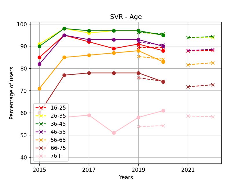
KTH BACHELOR THESIS REPORT. INDUSTRIAL MANAGEMENT AND ENGINEERING AND COMPUTER SCIENCE. JUNE 2021.                                     2

the internet in general, had to get familiar with the internet and        •  What effects on online shopping can be seen from the
start to explore the possible benefits of online stores and other            perspective of the 2020 pandemic?
internet services. One example is the senior citizens, wherein             • What differences can be identified between different
Sweden one out of ten tried online shopping for the first time               forecasting models when applied to a limited time series?
during the year 2020 [4]. Furthermore, Sweden experienced                  2) Hypothesis: The hypothesis is that based on the given
an increase in e-commerce, as the annual sales revenue from             historic data regarding e-commerce it is possible to make
e-commerce grew by 40% during 2020 [5].                                 well-based predictions that can be used as a basis for market
                                                                        analysis.
A. Problem
   One problem closely connected to commerce and e-                     C. Stakeholders
commerce is for companies to find suitable communication                   The expected outcome of the report is multiple forecasts of
channels to reach the consumer. The solution for this problem           the future trend of online shopping in Sweden in general and
is often market analysis and segmentation of the market.                over different demographic groups.
   When creating and designing a product, companies have                   This is of interest to all companies who conduct business
one or more specific groups of consumers in mind. Thus, it              where the consumer is an end-customer, regardless of whether
becomes essential to find those consumers and likewise, it is           the company is operating from physical or online stores
essential to know how to reach them. A market analysis can be           today. Companies need to be where the customers are, and
conducted in various ways, and one approach is to attempt to            the general trend among companies should be to meet the
predict the future shopping behaviour of consumers. By doing            customers on the internet. Few companies are completely
so, companies can better understand how and where to launch             unaffected by the transition towards everyday use of internet
new products for them to be successful with the consumer. In            in the daily life. Lack of execution or strategies for using the
the case of this report, the behaviour subject to prediction            internet to reach customers will likely result in the company
is online shopping. That is, companies need to be able to               losing significant market share. Thus, companies can benefit
predict the rate at which different groups of consumers shift           from the findings of this report to increase the understanding
to online shopping, what groups already have transitioned to            of the consumers, as well as by using the information about
e-commerce and what groups will take more time to transition.           possible trends when targeting customers.
   To make this prediction of consumer behaviour, the pro-
posed approach consists of machine learning algorithms and
regular regression. The reason behind implementing multiple             D. Sustainability
models is the fact that prediction models are difficult to                 The report and its findings have the potential to contribute
evaluate due to the lack of future data to compare to. By               to several of the UN:s goals of sustainable development.
implementing multiple models it is possible to compare the              No. 9 ”Build resilient infrastructure, promote inclusive and
predictions and thereby evaluate the performance of each                sustainable industrialization and foster innovation”, no. 11
model.                                                                  ”Make cities and human settlements inclusive, safe, resilient
   One of the main challenges with building an accurate model           and sustainable” and no. 12 ”Ensure sustainable consumption
is the limitations of the available data. In the case of this report,   and production patterns” to mention some. [6]
the data consist of a shorter time series, which makes the data            All the above-mentioned goals can be related to sustainable
sparse.                                                                 industry and sustainable consumption, which can be facilitated
                                                                        by e-commerce. Consumers no longer have to partake in
B. Purpose                                                              unsustainable ways of travel to reach stores, instead, they can
                                                                        go online. Therefore, even if the distribution of bought goods
   The report will investigate mainly two aspects of consumer
                                                                        is done via less sustainable ways, the net effect of greenhouse
and e-commerce in Sweden: what general trends can be
                                                                        gas emissions is reduced. Also, previous shopping areas, malls,
identified and what differences between different demographic
                                                                        large parking lots and other areas built for stores can be used
groups can be seen in their approach towards online shopping.
                                                                        for better purposes and the need for deforestation to build new
   The result of the investigation can then be used as a basis
                                                                        such areas disappears.
for market analysis. Companies involved in e-commerce or
attempting to enter the online market can use the findings
to increase their knowledge about what demographic groups                                     II. BACKGROUND
are potential consumers. The results could also be used to              A. Market Analysis
improve the understanding of the consumer and how to target                For a company to create successful marketing strategies,
them.                                                                   understanding the market in terms of the consumer,
                                                                        competitors, distributors and suppliers etc. is essential. To
  1) Scientific questions:                                              gain this understanding, there are many tools available
  • What differences in consumer behaviour are seen when                (for example SWOT, PESTLE, Ansoff-matrix) that help
    comparing different demographic groups (geographic lo-              the company analyse the internal and external environment
    cation, education, age and work sector)?                            as well as the consumer. When the market analysis has
  • What future trends in e-commerce can be identified?                 been conducted, the company can build on the discovered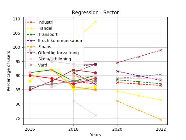
KTH BACHELOR THESIS REPORT. INDUSTRIAL MANAGEMENT AND ENGINEERING AND COMPUTER SCIENCE. JUNE 2021. 3
background knowledge to adjust the business idea and With b being the coefficients and " the random error which
formulate a business strategy, where the goal is to appeal assumed to be independent between the input values, x, and
to the consumers to make them paying customers. The normal distributed according to " ⇡ N (0, 2 ) [9].
consumer is often identified by consumer analysis and market By increasing the order of k, the equation can fit the training
segmentation. When the market segment is known, the data better. Finding the optimal degree of the polynomial can
company can create and launch efficient marketing campaigns be done by Forward Selection, where k is increased until the
specific to the segment. [7] optimal value is found. The coefficients can also be optimized,
which makes it possible to get the equation that fits well
1) Segmentation: The goal for companies is to offer a prod- to the data. The optimization of the degree of polynomial
uct to meet customer demands. However, the problem is that and coefficients can be done in multiple ways, but the most
there are too many customers for one company to cater to each straightforward approach is to minimize the error measured as
of their individual needs. The solution is therefore to cluster Mean Square Error (MSE). [10] See equation (9) in Appendix
customers with similar demands and process the demands of B.
the cluster instead, i.e. segmentation. After a conducted market
segmentation, the company can use strategies to analyse the
segments in terms of growth, competitors and size to determine C. Support Vector Regression
what or which segments to focus on. The above-mentioned Support Vector Regression (SVR) uses the idea behind
factors all influence the profitability of the segment and how Support Vector Machine (SVM) and applies it to regression
to best target consumers. problems (see Appendix VIII-B for SVM). The model can also
Furthermore, when the target groups of customers be used for the prediction of unseen data. To solve non-linear
have been identified via segmentation, the company can regression problems, the technique for mapping the non-linear
conduct further consumer analysis to gain an even better data with the kernel trick is used, just as for a regular SVM.
understanding of the customer and segment. The choice of Given data points (x1 , y1 )...(xn , yn ), the goal of the model is
communication and platform to target the consumer are key to find the optimal function to map the input values, x, to the
factors for successful marketing. Therefore, the company corresponding target, y.
need to explore what is the best-suited platform and how to The main difference between SVR and SVM is the loss
communicate the message of the product to the consumers. [7] function used, which has to be changed to solve regression
problems. There are a few different loss-functions such as
2) Forecasts: There are also certain difficulties connected Laplace-, Huber’s Gaussian- and "-sensitive loss-function.
to forecasting in general which needs to be considered when Among these, the "-sensitive loss function is the most com-
companies attempt to predict the market or consumer be- monly adopted. [11] See equation (10) in Appendix B.
haviour. First, a suitable period should be chosen, the longer The loss function is equal to 0 only if the data point is
the time span of the forecast the more uncertain it gets. Second, within the pre-determined radius of the predicted line. Since
limitations of data, time or resources also add constraints to the loss function is subject to minimization, the model will
the forecast. If any of the mentioned variables are scarce, one seek to avoid any data points outside the radius when finding
should preferably use time series analysis, which models time a solution. Thus, the optimal solution will have the majority
as the independent variable. Thus, the forecast is limited to of the data points within the radius. [11] See Figure 4 in
show correlations and trends. However, for the purpose of the Appendix A for an illustration of a simple SVR.
report, correlations and trends are just what is needed. Third, The generic function of SVR with the kernel function can
complex methods are not necessarily preferred over simpler be written as f (x) = (w ⇤ (x) + b). The most common
ones. Simple models are less sensitive to inaccuracies in the kernels are Gaussian RBF: (x, xi ) = exp( ||x2 2xi || ) and
2
data or the model compare to more complex ones. However, the polynomial kernel: (x, xi ) = (xTi ⇤ x c)p . With
a model can also become too simple and overlook important respectively p the parameter to tune. The minimization of the
factors or miss correlations. Thus, there is a trade-off between regression risk can thus be expressed as:
simple and complex models to be considered. [8]
X n
1
Rreg (f ) = |W |2 + C (⇣i ⇣i⇤ ) (2)
2
B. Polynomial Regression i=1
Regression is one of the most commonly used tools for Subject to:
forecasts and identifying correlations between variables. The
( qi (w ⇤ (xi )) b " + ⇣i
most fundamental approach is simple linear regression, which
can model linear predictions and identify the relation between (w ⇤ (xi )) + b qi " + ⇣i⇤ (3)
input values, x, and the target values, y, as a straight line. ⇣i⇤ , ⇣i 0, for i = 1, ..., n
The more general model is nonlinear or polynomial regression
which can model more complex relations. The model allows Where Rreg is the function to minimize, with the constraints
one to fit an equation of the k:th order to the data: defined above. The variables to tune, which is done by the user,
are " (the radius or allowed deviation), C (slack or training
Y = b0 + b1 x1 + b2 x22 + ... + bk xkk + " (1) error) and (kernel function). [12], [13]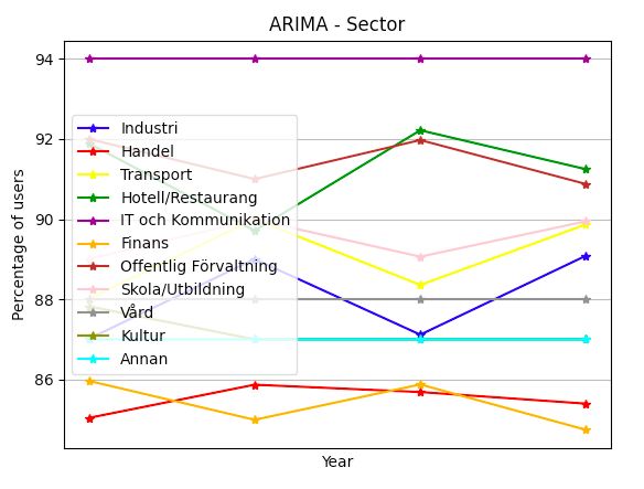
KTH BACHELOR THESIS REPORT. INDUSTRIAL MANAGEMENT AND ENGINEERING AND COMPUTER SCIENCE. JUNE 2021.                                              4

D. ARIMA                                                                        is preferable to set the parameters conservatively to avoid over-
   Autoregressive Integrated Moving Average (ARIMA) is a                        differentiation. To fix potential over- or under-differentiation
statistical analysis model which uses time-series data to predict               it is possible to add either an additional MA or AR term. [15]
future trends. An ARIMA model is, by standard, characterized                       When the ARIMA model is built it can be favourable to
by three parameters p, d and, q.                                                optimize it using out-of-time cross-validation, which is done
   p represents the order of the Auto Regressive term or the                    by looking back at previous data points and using them to
lag order, also known as the number of lag observations in the                  forecast as many steps back that were taken. These forecasted
model. q is the size of the Moving Average window. The last                     points are then compared to the actual ones for that time. See
parameter is d, which is the number of times the observations                   Figure 5.
are differenced. When d = 0, the series is already stationary.                     As the different parameters are selected for the model the
[14]                                                                            prediction will look similar to Figure 6. Additional fine-tuning
   In the Auto Regressive model (AR), the function is, as                       can then be done to match the observed values to predicted
previously mentioned, only dependent on its lags and the                        values more precisely.
equation looks as follows:
                                                                                E. Data set
               Yt = ↵ +       1   ⇤ Yt      1   +    2   ⇤ Yt     2
                                                                          (4)      The data consists of the annual survey done by Internetstif-
                              +... +            ⇤ Yt         + "1
                                            p            p
                                                                                telsen, Svenskarna och Internet, which is a national survey
Where ↵ is the intercept term and is the coefficient of lag                     about the use of the internet in Sweden. The data from
that the model estimates.                                                       the reports are aggregated by the possible responses to each
   Similarly, in the Moving Average model (MA), the function                    question. One of the questions in the survey concerns online
is dependent only on the lagged forecast errors.                                shopping behaviour. That is, the data shows the share of users
                                                                                of e-commerce in Sweden in a specific year.
             Y t = ↵ + "t +        1   ⇤ "t     1    +   2    ⇤ "t    2            The survey also provides multiple demographic variables,
                                                                          (5)
                                            +... +       q ⇤ "t       q         where the ones chosen for this report are geographic location,
                                                                                education, age and work sector. The data spans from the year
The error terms are the errors of the auto-regressive models
                                                                                2000 to 2020 and from 2015 to 2020.
(see above) of the respective tags. For example, the error "1
is the error of the following equation:
                                                                                F. Prediction of very short Time series
                 Yt =     1   ⇤ Yt     1   +     2   ⇤ Yt     2
                                                                          (6)      The dilemma of insufficient data is one of the most common
                              +... +        0   ⇤ Y 0 + "t                      problems encountered when attempting to model a forecast
So, the ARIMA model combines these two terms and differ-                        or build any model based on historic data. In theory, the
entiate the series to make it stationary, i.e. the equation can                 number of data points needs to be greater than the number of
be written as:                                                                  parameters of the model. However, the number of data points
                                                                                needed is often a lot more than what the theory suggests. [16]
            Yt = ↵ +          ⇤ Yt         +         ⇤ Yt         + ...
                          1            1         2            2
                                                                                   In the best scenario, there is enough data to both train
                      +   p   ⇤ Yt      p   ⇤ "t +        1   ⇤ "t    1   (7)   and test the model on unseen data. This is not possible with
                     +    2 ⇤ "t       2 + ... +          q ⇤ "t      q         limited data. One way to increase the available training data
                                                                                is by n-fold cross validation. Because the model’s purpose
To use the model, the hyperparameters need to be determined.                    is forecasting, the training data should always be before the
The purpose of d is to make the time series stationary.                         test data when put on a timeline, which adds a restriction.
However, there is also a risk of over-differentiating, which                    One method of cross-validation which can be used and takes
will affect both the parameters and the outcome. To find the                    the restriction into concern is rolling-origin-recalibration
correct value of the parameter it is important to identify the                  evaluation.
minimum difference to get a relatively stationary series, where
the autocorrelation function (ACF) plot reaches zero quickly                       1) Rolling-origin-recalibration evaluation: By taking a
and the mean roams around a set value. [14]                                     small subsample of the available data as training data, the next
   To determine the order of the parameter p (AR term) it is                    sample or subset can be the training subset’s test data. At the
important to identify if the model needs it, and then determine                 next step, the test data is added to the training subset and the
it by using the partial autocorrelation function (PACF) plot.                   following data point or subset is the new test data. This way
PACF finds the correlation of the residuals with the next lag,                  of dividing the data into training and test data can be done
unlike ACF which finds the correlation of the present with                      throughout the available data. The accuracy of the model will
past lag. The value of p is then determined to be the lag value                 be the average computed accuracy at each step [17].
where the PACF plot crosses the upper confidence level the
first time. [15]
   The order of q (MA term) is obtained from the ACT plot.                      G. Related Work
The information is found where the plot crosses the upper                         Multiple studies have been done to examine SVR and
confidence level and its corresponding lag value. Generally, it                 the models’ capabilities. The majority of studies have shown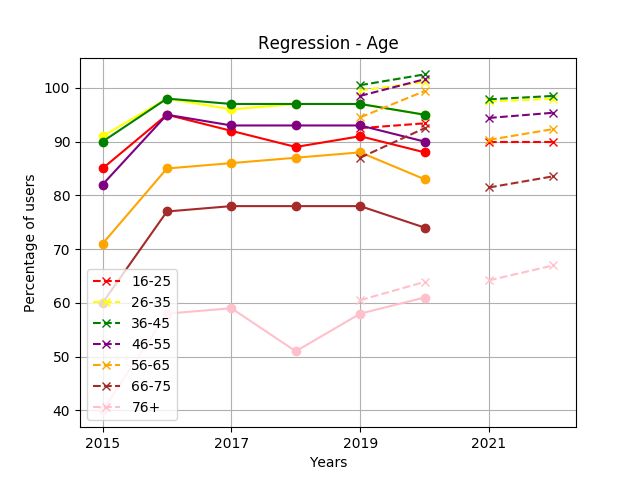
KTH BACHELOR THESIS REPORT. INDUSTRIAL MANAGEMENT AND ENGINEERING AND COMPUTER SCIENCE. JUNE 2021.                                  5

positive results regarding forecasting models based on the al-        B. Implementation
gorithm, thus the general conclusion is that the model performs          The models are built in Python using standard libraries such
satisfactorily. SVR has been used to forecast different time          as NumPy, Scikit-learn, and Matplotlib.
series such as the stock market [11], [18], energy consumption           Each model was optimized by iteratively changing the
[19] and other time series [20], [21].                                values of the hyperparameters. For each model, MSE was
   As mentioned by U. Thissen et al. SVR has multiple                 computed and the optimal model was defined as one with
advantages making the model attractive to use. Especially the         the lowest average MSE score. When the optimal model was
model’s generalization capabilities combined with the ability         found, the values of the hyperparameters were noted and the
to always find a unique and sparse solution which also is the         model predicted the future e-commerce. This was repeated for
global solution [20]. The model can also be used for data with        the different data sets.
multiple features which is shown in the study regarding energy           The forecasts and computed MSE was compared to each
consumption [19]. Furthermore, the same article uses n-fold           other as a method of evaluation since there is no way to eval-
validation when training the model, which indicates that the          uate a forecast. To identify differences within demographics,
approach to handle limited data and hyperparameter selection          multiple predictions were made. One for each demographic
with n-fold validation is suitable for SVR.                           group.
   The 1998 study “The use of ARIMA models for reliability               Additionally, the accuracy of the models was computed
forecasting and analysis” comes to the conclusion where               to further evaluate how well the different approaches to the
Ho and Xie claim that the model is very flexible and give             problem fit the historic values and forecasted the future. The
statistically accurate predictions, something which has been          accuracy was calculated as:
accepted since the model is widely used for forecasting today
[22]. This is supported in the Babai et al. 2013 article where                                    Actual F orecast
they forecasted the demand in a two-stage supply chain. The                 P ercentageError =                         ⇥ 100 (8)
                                                                                                         Actual
publication reaches the same conclusion that the model is both
                                                                        Some of the demographic groups had little data or missing
efficient and accurate. This study is also more relevant seen
                                                                      data points. This was dealt with by excluding the groups the
from the perspective of this report, as it also investigates future
                                                                      model did not have sufficient data for to make a forecast.
trends [23].
   In the 2016 article “Gold Price Forecasting Using ARIMA               1) Polynomial Regression: By implementing forward
Model” Guha and Bandyopadhyay use ARIMA for predicting                selection with the start at an equation of order p = 1
the price of gold. This article is, as the one previously             (assuming the data to be non-linear), the degree of the
mentioned, more in line with what this report will investigate        polynomial was increased iteratively. The maximal possible
which gives insight into both opportunities and limitations of        order of the polynomial is n 1 where n is the number of
the model. The report explains how the model is applied and           data points. At each step, MSE was computed.
the limitations, one of which is that it might be more suitable
for predicting values in the near future, something that was             2) Support Vector Regression: The model used the "-
not mentioned in earlier reports but is important to take into        sensitive loss function to compute the cost function and the
consideration. [24]                                                   Gaussian RBF kernel function for modelling data to a higher
                                                                      dimension. The values of hyperparameters C, respectively the
                                                                      allowed deviation ", was optimized by systematically testing
                         III. M ETHOD                                 different values and computing MSE.
   The study consisted of data pre-processing, implementation
                                                                         3) ARIMA: Initially, the PACF and ACF plots were used
and parameter optimization for each model, and lastly predic-
                                                                      to delimit the possible parameters. This guideline was then
tion and evaluation of the models. The models implemented
                                                                      used to optimize the implementation of the model by testing
were polynomial regression, SVR and ARIMA.
                                                                      different values of the three hyperparameters. The model was
   The findings, that is the forecasts, of the different models,      then optimized by using out-of-time cross-validation.
were evaluated in terms of being suitable as a part of a market          The accuracy was computed as MSE over the last step.
or consumer analysis.
                                                                      C. Limitations
A. Data Pre-processing                                                   The data set could be considered small since it consisted
                                                                      of 20 data points at the most. To handle the problem with
   The data from Internetstiftelsen was transformed into a            limited data, rolling-origin-recalibration evaluation was used.
format compatible with the models and modelled as a time              The data was divided into smaller subsets with only a few data
series. x(t), t = 1, 2, ..., n with each value of x, year, having     points in each subset. The general forecast had 4 subsets of
a corresponding target value, y, percentage of users.                 5 points, while the different demographics had a test set that
   Further processing of the data was made for the different          consisted of the 2 last data points and the prior data points
representations of the data, where each representation repre-         made up the training set. MSE was computed as the average
sents a certain demographic.                                          MSE.
KTH BACHELOR THESIS REPORT. INDUSTRIAL MANAGEMENT AND ENGINEERING AND COMPUTER SCIENCE. JUNE 2021. 6
The forecast of the future was set to the time horizon forecasts also gave unrealistic results with values over 100%
of two years ahead, 2021 and 2022. The choice of such a during the training phase, which can be seen as a limitation
short forecast was based on the high degree of uncertainty that comes with the simplicity of the model.
concerning the future. For a field like the internet, which is
characterized by rapid change in technology, one can assume
the future of e-commerce to be more uncertain than other,
historically more stable fields. Thereby a short time horizon
was chosen, to limit the amount of uncertainty.
Furthermore, the models did not consider the fact that
the population percentage cannot exceed or equal 100%, and
thereby gave predictions of values over 100%. These values
could be achieved because of the simplicity of the models, but
cannot occur in reality. For cases where the predicted value
was over 100, we disregarded the actual value and instead
Fig. 1. Forecast over all data points for the regression model. The 2:nd degree
acknowledge the trend as strongly increasing and being close curves are clearly visible.
to 100%. All values were however included in the graphic
representations. Removing the data point of 2020 from the training data
made the slope of the prediction steeper, that is the trend
IV. R ESULT declined faster. See Figure 7 and 8. However, the value for
Below we will highlight the most interesting findings. As the 2022 only differed by 1% between the two forecasts (see Table
data concerns the share of users of e-commerce, all predicted III in IX-A).
values will thus represent the share of users for a specific The majority of the forecasts over the demographics showed
year. For values in tables and graphs over the forecasts, see a stable or slightly increasing trend. Only one group, Finans
Appendix IX. from the work demographic showed a strong declining trend
General findings were that the general forecast for all three with a drop of about 10 percentage points.
models showed a declining trend, see Table I below. The MSE for the model differed highly between the data sets.
models also forecast the elderly and people living in the The predictions over demographic groups had a lower MSE
countryside to increase their use of e-commerce over the next compared to the general model. This is probably since the gen-
few years. eral model had more data points to measure. The percentage
error was also quite varied, see Table II in IX-A.
General Prediction 2021-2022
Year Polynomial SVR ARIMA
Regression B. Support Vector Regression
2021 81 83 84 The general forecast showed a downward trend which is
2022 77 77 79
quite steep. Over the years 2020-2022 the number of users
TABLE I
OVERVIEW OF THE GENERAL PREDICTION DONE BY THE DIFFERENT
decrease by 10 percentage points, measured as the difference
MODELS FOR YEAR 2021-2022 between the actual value of 2020 and the forecast of 2022.
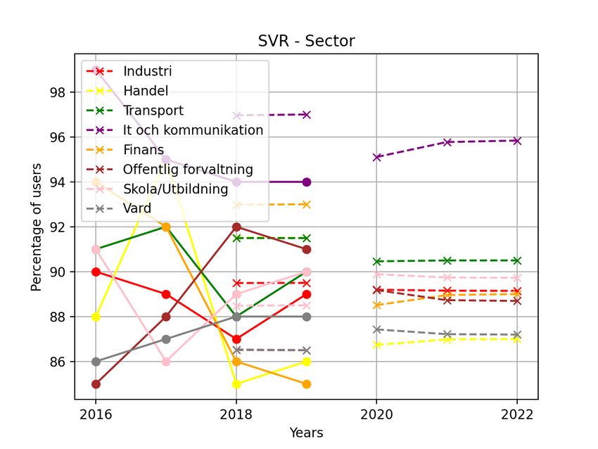
The result of the forecasts over the different demographics
is quite different from the general trend since they all have
The removal of the data point of 2020 showed little impact a more or less straight trend for the years 2021-2022. Some
on the forecasts. For the years 2021 and 2022, the change in of the forecasts showed a slight increase or decrease over the
training data mostly affected the slope of the forecast. The period 2020-2021 but then a stable trend (see Figure 2).
predicted values for the coming years are quite similar with
or without the last data point for all forecasts.
A. Polynomial Regression
The general forecast showed a declining trend over the next
years, where fewer consumers will use online shopping. The
forecast decreases by 10 percentage points over the years
2020-2022, measured as the difference between the actual
value of 2020 and the forecast of 2022.
Furthermore, it is clear how the model is influenced by
historical data and the degree of the polynomial. The general Fig. 2. Forecast over the segment based on age. The future trends for all
model is of the second degree, and when visualizing the subgroups are straight or slightly increasing.
forecast the curves of a second-degree polynomial are visible
(see Figure 1). Likewise, the majority of the demographic In general, the model does not fit very well to training data,
forecasts are of the first degree, something that also can see Figure 13 and 14. The forecasts for the general model
be seen by the straight lines which are the forecast. Some done during the training phase are not close to the actualKTH BACHELOR THESIS REPORT. INDUSTRIAL MANAGEMENT AND ENGINEERING AND COMPUTER SCIENCE. JUNE 2021. 7
values, which also can be seen by the high MSE of the model was quite high relative to other values. For example, some
or by the large difference between predicted and true values subdivisions in the sector demographic had a much higher
(see Table V IX-B). However, MSE-score for the demographic MSE than others in the same group (see the MSE for Annan
groups are much lower and some values can be considered vs Skola/Utbildning). Additionally, the percentage error of the
satisfactory. Similarly, the percentage error of the model differs general forecast, as well as the different demographics, showed
quite a lot when comparing the general forecast to the average small errors from the historic data points. See table IX-C
demographic forecast.
Moreover, the removal of the data point of 2020 had V. D ISCUSSION
little influence on the forecast and gave results in line with The different models resulted in quite different forecasts,
the results from the regression model. The forecasted values in some cases even contradictory of each other. The varied
before 2020 were the same even after removing the data point. results illustrate the uncertainty of prediction models and how
However, the predicted values after 2020 showed almost no the forecast is dependent on the chosen model.
difference at all compared to the forecast with all data points. The investigation of the report and its results did offer
The value predicted for 2022 was the same and for 2021 there predictions for the future of e-commerce which can be used
was only a 1% difference between the predictions. as a basis for market analysis. However, as the three different
models also produced deviating results, it is quite difficult
C. ARIMA to do a market analysis based only on the produced results.
In general, the ARIMA model predicted a negative trend Instead, it might be possible for companies to draw some
as seen in Figure 18. With the removal of the data point of conclusions regarding a possible behaviour but the results
2020, the forecast behaved similarly to the forecast with the are not strong enough to base the market analysis on alone.
data point. However, the declining trend was not as steep, see Furthermore, the models all show a higher accuracy when
Figure 20. investigating a smaller group, which indicates that the models
In contrast, the results from the different demographic are better suited for forecasting specific groups’ behaviour.
groups differed, as some predictions increased while others
decreased. As seen in Figure 3, the predicted values for people A. Effects from the pandemic
living in the countryside were lower in the year 2021 compared Looking at the data set on which the models are built, it
to 2020. This value is expected to rise the following year. By is clear that during the height of the pandemic in 2020 e-
observing the same graph, the prediction for those located in a commerce dropped by several percentage points, something
city shows the opposite, as the percentage is expected to first that was quite unexpected given the circumstances. As local
rise in 2021 and then fall the following year. restrictions meant that many people refrained from shopping
in physical stores and many malls and stores decreased their
opening hours, it was reasonable to think that consumers might
have turned towards e-commerce. However, as previously
mentioned, this was not the case, which leads us to other
possible explanations as to why e-commerce decreased in
2020.
One natural explanation is the fact that many people lost
their jobs or were laid off short-term, which meant less income
to dispose of. Another reason is that the purchases of services
(tickets, travels etc.) online has drastically decreased as events
have been cancelled and travels were largely restricted both
nationally and globally, a product group that previously made
up a large portion of the total e-commerce. Furthermore,
Fig. 3. Forecast over the segment based on location of living. The forecast the data do not include the occurrence of online shopping
of those living on the countryside is seen increasing in 2022.
or monetary aspects which can result in the forecasts being
Another demographic group where the prediction is a per- misleading.
centage increase is the group under education which have only Thereby, the general prediction, which showed a declining
finished Grundskola. The model predicted higher percentages trend, can be deceiving in the sense that e-commerce for
for both 2021 and 2022, which can be seen in Figure 23. certain customer groups and certain product groups increased.
Most age groups showed a relatively stable forecast with Individuals already familiar with online shopping increased
values close to the ones from previous years. However, 76+ the number of purchases done via the internet, while other
showed a decrease in percentage for the year 2021, which then groups of individuals decreased their overall purchases and
rose again in 2022, similarly to the forecast for those living accordingly also decreased their online shopping.
in the countryside. See Figure 21.
In general, the model produced forecasts which fit well B. Demographic groups
for the existing data points. Although, as seen in Table V The different models sometimes resulted in contradicting
in IX-C, some demographics were less accurate as the MSE forecasts for a certain demographic, which makes it hardKTH BACHELOR THESIS REPORT. INDUSTRIAL MANAGEMENT AND ENGINEERING AND COMPUTER SCIENCE. JUNE 2021. 8
to draw solid conclusions about the future trend for that First, the complexity of the behaviour subject for prediction
demographic. However, the forecasts also seemed to agree on decides what model is suitable. A more complex model will
the trend of other demographics, for example, age. optimize itself to historical data and past trends have a large
We can see that the general finding for the elderly in Sweden influence on the shape of predicted trends. While a simple
is an increase in e-commerce since the three groups 56-65, 66- model is more general, but faces the risk of being too general
75 and 76+ all showed increasing trends. Thus, these groups and thus miss to model important relations.
will likely be more present on the internet in the future. This Second, the data available has to be considered. The re-
is probably the effect of the pandemic, where individuals gression model is bound by the constraint of the degree of
have to get more comfortable with the different tools offered the polynomial, that is, there is a limit of the degree which
by the internet due to offices encouraging working from limits the possible relations the model can portrait. ARIMA
home and restrictions for senior citizens regarding socializing has a minimum number of data points needed for training
with others. Another explanation might be that the younger data which adds a constraint to the data set being used as
generation, consisting of people who already have embraced training data. SVR, on the other hand, has not the same
technology and internet solutions, in the near future will enter constraints concerning training data, but many possibilities of
the group of elderly in Sweden. Thereby, the groups’ general hyperparameters to fine-tune which can be time-consuming.
habits concerning the internet will change accordingly. Despite the model chosen as a tool for creating marketing
When dividing data after the demographic of the degree strategies, the results have to be used with caution and
of education, the majority of the models show an upwards- rationality as all models come with risks of not being truly
sloping trend for the group of Grundskola. Assuming the representative and are flawed in some way.
majority of people with a low level of education belong to
the part of the workforce with lower income, the jobs they
occupy are the ones employers cut first when money becomes D. Further Improvements and Research
tight for the company. Due to the previous slow growth in The report investigated the share of users of e-commerce
Sweden of 2019 and the pandemic in 2020 many low-income and one interesting aspect to further research would be the
jobs disappeared resulting in the declining trend. annual turnover of e-commerce. The turnover can be a good
However, the predictions show this trend being turned complement to this report as the number of users alone cannot
around. Based on the estimates of these trends and history, show the whole picture of a market or segment. By having in-
when the economy recovers the jobs previously dismissed will formation about both the share of potential consumers and the
be reinstated. As a result of the decrease in unemployment, expected turnover, companies can form a well-based market
people have more income to dispose of and thereby money to analysis.
spend on e-commerce. For this report, the data used to build the models was
Additionally, when investigating the groups of individuals aggregated. One interesting aspect for further investigation
living in the countryside the models agree on an upwards trend would be to have non-aggregated data, to create models for
for the coming years, something that can be interesting to more specific groups instead of the more general ones used
investigate further. The different models based on the work in this report. As the study was performed on the market as
sector contradicted each other and thereby gave inconclusive a whole, with some larger demographic groups, the result can
forecasts. mostly be used to get a general picture of the market, and
One general conclusion which can be drawn from the gath- the under-laying trends, for the next few years. For a specific
ered demographic forecasts is that the MSE and percentage company, it could be more rewarding to look into their specific
error is lower compared to the general forecasts. This indicates target groups, if they are more delimited.
that the models perform better and thus are more accurate Generally, the lack of data is often a problem in these
when forecasting the behaviour of a smaller group. reports, as the results might be lacking when there are limited
observations to take into consideration. As this report did
C. The Models not handle a large data set, it could be interesting to further
The majority of forecasts modelled by ARIMA resulted in research the future trend of e-commerce, using more data
oscillating predictions and a low MSE. This can be seen as points and thus being able to predict a, possibly, more accurate
a result of using a complex model to predict a future with forecast.
a lot of uncertainty in the form of unpredictable variables. Moreover, while it is possible to conclude that the models,
On the other hand, the regression model was often built on a in general, perform better on a small group of individuals
low degree of the polynomial and therefore resulted in models the measurements are not weighted after the number of data
with good generalization capabilities. However, the nature of points. Since the general models are based on more data,
the low polynomial also made it possible for the forecasts to the lower accuracy can just be the result of having more
predict unrealistic values. data points to measure. Or that the fewer data points of
The optimal model of the three implemented to forecast the demographics make it easier for the models to learn the
consumer behaviour in terms of marketing purposes is hard pattern of the data and not get truly generalized. Thus, one
to determine. However, the findings from the report can offer improvement to be made and a research subject would be
some guidelines and features of the models to be considered to gather more data from the demographics and measure the
when choosing a model. differences in accuracy compared to the general models.KTH BACHELOR THESIS REPORT. INDUSTRIAL MANAGEMENT AND ENGINEERING AND COMPUTER SCIENCE. JUNE 2021. 9
Concerning the models, specifically the regression model, We would also like to thank our supervisors from KTH for
the forecasts could be unrealistic (predicting a value over the support they have given us. As well as our peers, thank
100%). One improvement to be made to get more realistic you for the reviews.
values would be to put a constraint on the model, to approach
the value of 100 asymptotically. AUTHOR C ONTRIBUTIONS
Disa Nilsson Rojas currently a BSc student of Industrial
VI. C ONCLUSION Engineering and Management with specialization in computer
Based on the results of the models, the general predictions engineering at KTH. The author contributed mainly to the
show a declining future trend of e-commerce with fewer polynomial regression and SVR models, as well as part I,
individuals turning to online stores. While the results show IV-VI.
one thing, it is also important to take into account the increase Freja Engström currently a BSc student in Industrial En-
in revenue e-commerce experienced during 2020. It would gineering and Management with a specialization in computer
thereby not be wise to only look at the results of this study, engineering at KTH. The author contributed mainly to the
since the interpretation of declining e-commerce might not be ARIMA model, as well as part I, IV-VI.
the reality. Instead, other aspects should be incorporated into
market analysis, such as the total sales revenue. R EFERENCES
The report also shows some evidence of how the results can
be misleading and give a wrongful picture. When investigating [1] L. Zhou, L. Dai, and D. Zhang, “Online shopping acceptance model-
a critical survey of consumer factors in online shopping,” Journal of
different demographics the majority of the forecasts show the Electronic commerce research, vol. 8, no. 1, p. 41, 2007.
opposite trend from the general forecast, and therefore the [2] EuroStat. Share of enterprises’ turnover on e-commerce.
general model can be seen as too generalized and poorly [Online]. Available: https://ec.europa.eu/eurostat/databrowser/view/
tin00110/default/line?lang=en
representative. Furthermore, the results from the models show [3] C. Katawetawaraks and C. Wang, “Online shopper behavior: Influences
that there are differences within a certain demographic group of online shopping decision,” Asian journal of business research, vol. 1,
in their approach to e-commerce, which has to be considered no. 2, 2011.
[4] InternetStiftelsen, “Svenskarna och internet 2020,” Svenskarna och in-
by a firm but are missed in the general forecasts. While some ternet, pp. 44–55, 2020.
groups in society have reduced their online shopping, others [5] H. R. Postnord, Svensk digitalhandel, “E-barometern helårsrapport
increasingly used the internet for their purchases. For example, 2020,” E-barometern, p. 5, 2020. [Online]. Available: https://media.
dhandel.se/wl/?id=x8VMpPpkiZRvhD0a75bKwplEPMsAl3gp
many elders made their first purchase online during 2020. [6] U. D. of Economic and S. Affairs. The 17 goals. [Online]. Available:
During the same period e-commerce for people with Grund- https://sdgs.un.org/goals
skola level of education dropped. This shows that different [7] L. Mossberg and M. Sundström, Marknadsföringsboken. Studentlitter-
atur, 2011.
groups will react differently to the same events and therefore [8] A. Feldmann, “Forelasning 4 - prognoser in me1316,” January 2020.
it is important to investigate the target audience of a company [9] A. Agarwal. Polynomial regression. [Online]. Available: https:
instead of the general picture. //towardsdatascience.com/polynomial-regression-bbe8b9d97491
[10] Abhigyan. An introduction to support vector regression
Thus, the conclusion is that while the models can show a (svr). [Online]. Available: https://medium.com/analytics-vidhya/
possible forecast, more information is needed to conduct a understanding-polynomial-regression-5ac25b970e18
market analysis. [11] C.-J. Lu, T.-S. Lee, and C.-C. Chiu, “Financial time series forecasting
using independent component analysis and support vector regression,”
As for the use of these models to gain knowledge of the Decision Support Systems, vol. 47, no. 2, pp. 115–125, 2009.
market and use the information for marketing purposes, the [Online]. Available: https://www.sciencedirect.com/science/article/pii/
models come with different pros and cons. The decision of S0167923609000323
[12] B.-J. Chen, M.-W. Chang et al., “Load forecasting using support vector
the model should be based on the available data and the machines: A study on eunite competition 2001,” IEEE transactions on
trade-off between simplicity and complexity. Furthermore, power systems, vol. 19, no. 4, pp. 1821–1830, 2004.
the models seem to be more accurate in their forecasts of [13] M. Awad and R. Khanna, Support Vector Regression. Berkeley, CA:
Apress, 2015, pp. 67–80. [Online]. Available: https://doi.org/10.1007/
certain demographics compared to the forecast including the 978-1-4302-5990-9 4
entire population. The conclusion is thereby that the models [14] S. Prabhakaran. Arima model – complete guide to time series forecasting
implemented in this report give more accurate forecasts when in python. [Online]. Available: https://www.machinelearningplus.com/
time-series/arima-model-time-series-forecasting-python/
modelling a certain, smaller target group. Companies can [15] J. Salvi. Significance of acf and pacf plots in time series
thereby use the models to predict the behaviour of certain analysis. [Online]. Available: https://towardsdatascience.com/
segments of the market. significance-of-acf-and-pacf-plots-in-time-series-analysis-2fa11a5d10a8
[16] R. J. Hyndman and G. Athanasopoulos, Forecasting: Principles and
Practice. OTexts: Melbourne, Australia, 2018, ch. 12.7.
ACKNOWLEDGMENT [17] ——, Forecasting: Principles and Practice. OTexts: Melbourne,
Australia, 2018, ch. 3.4.
We are grateful for the opportunity to research and inves- [18] P. Meesad and R. I. Rasel, “Predicting stock market price using support
vector regression,” in 2013 International Conference on Informatics,
tigate the area of e-commerce, which we find interesting and Electronics and Vision (ICIEV), 2013, pp. 1–6.
of relevance. [19] Z. Ma, C. Ye, and W. Ma, “Support vector regression for predicting
We thank Internetstiftelsen for providing the data from their building energy consumption in southern china,” Energy Procedia,
vol. 158, pp. 3433–3438, 2019, innovative Solutions for Energy
annual survey, Svenskarna och internet, and especially our Transitions. [Online]. Available: https://www.sciencedirect.com/science/
supervisor Cia Bohlin. article/pii/S1876610219309762KTH BACHELOR THESIS REPORT. INDUSTRIAL MANAGEMENT AND ENGINEERING AND COMPUTER SCIENCE. JUNE 2021. 10
[20] U. Thissen, R. van Brakel, A. de Weijer, W. Melssen, and
L. Buydens, “Using support vector machines for time series
prediction,” Chemometrics and Intelligent Laboratory Systems, vol. 69,
no. 1, pp. 35–49, 2003. [Online]. Available: https://www.sciencedirect.
com/science/article/pii/S0169743903001114
[21] Chun-Hsin Wu, Jan-Ming Ho, and D. T. Lee, “Travel-time prediction
with support vector regression,” IEEE Transactions on Intelligent Trans-
portation Systems, vol. 5, no. 4, pp. 276–281, 2004.
[22] S. Ho and M. Xie, “The use of arima models for reliability forecasting
and analysis,” Computers Industrial Engineering, vol. 35, no. 1,
pp. 213–216, 1998. [Online]. Available: https://www.sciencedirect.com/
science/article/pii/S0360835298000667
[23] M. Babai, M. Ali, J. Boylan, and A. Syntetos, “Forecasting and
inventory performance in a two-stage supply chain with arima(0,1,1)
demand: Theory and empirical analysis,” International Journal of
Production Economics, vol. 143, no. 2, pp. 463–471, 2013, focusing
on Inventories: Research and Applications. [Online]. Available:
https://www.sciencedirect.com/science/article/pii/S0925527311003902
[24] B. Guha and G. Bandyopadhyay, “Gold price forecasting using arima
model,” Journal of advance Management Journal, 03 2016.
[25] T. Sharp. An introduction to support vector regres-
sion (svr). [Online]. Available: https://towardsdatascience.com/
an-introduction-to-support-vector-regression-svr-a3ebc1672c2
[26] M. Awad and R. Khanna, Support Vector Machines for Classification.
Berkeley, CA: Apress, 2015, pp. 39–66. [Online]. Available: https:
//doi.org/10.1007/978-1-4302-5990-9 3KTH BACHELOR THESIS REPORT. INDUSTRIAL MANAGEMENT AND ENGINEERING AND COMPUTER SCIENCE. JUNE 2021. 11
VII. A PPENDIX A model can always find an optimal decision boundary in some
dimension [26].
To increase the generalization capabilities the SVM also
has an additional parameter C or slack. The slack variable
allows for some misclassification which can be good because
the training data doesn’t always entirely represent the
actual distribution of data. This introduces what is called
a soft margin, which is used in cases where some points
need to be misclassified to find an optimal solution, i.e.
Fig. 4. Example of a simple SVR [25] decision boundary. As C increases, the less tolerance for
misclassification the model will have. If C instead is small,
the more tolerant the model will be.
1) Loss function: L" (f (x), q) =
(
|f (x) q| ", if |f (x) q| "
(10)
0, otherwise
Where " represents the the radius around the optimal hyper-
Fig. 5. ARIMA model with both historic data and forecast plotted [14] plane.
Fig. 6. Example of forecast vs actual values [14]
VIII. A PPENDIX B
A. Mean Square Error
n
1X
E= (predii yi ) 2 (9)
n i=1
B. Support Vector Machine
Support Vector Machine (SVM) is a classification model
and performs the task of classifying data points by finding
the optimal hyperplane, i.e decision boundary, in N-dimension
for separating the data points. The goal is to find a decision
boundary with respect to two criteria: the model should
generalize well on unseen data and thus classify all new data
points correctly. As well as being the decision boundary that
maximizes the margin (maximizes the distance between the
data points and the boundary). And while there might be
multiple solutions to a classification problem, there is only
one solution that fulfils both criteria.
To find this optimal decision boundary, and to be able to
solve problems that are seemingly non-linearly separable when
visualized, the SVM uses the kernel trick. That is, to map the
data onto a higher dimension. SVM uses the kernel trick be-
cause data points that are non-separable in a lower dimension
will become separable in a higher dimension. Thereby, theKTH BACHELOR THESIS REPORT. INDUSTRIAL MANAGEMENT AND ENGINEERING AND COMPUTER SCIENCE. JUNE 2021. 12
IX. A PPENDIX C
A. Polynomial Regression
Group MSE Error %
General 173.031 80.34
Age 16-25 7.852 7.78
26-35 10.865 9.00
36-45 17.125 11.50
46-55 41.202 18.80
56-65 77.802 27.15
66-75 105.813 36.54
75+ 3.667 9.06 Fig. 8. Forecast without 2020
City Stad 24.222 14.46
Landsbyggd 45.625 21.82
Education Grundskola 32.951 20.88
Gymnasie 3.086 5.81
Högskola 1.063 2.70
Sector Industri 1.250 3.40
Handel 204.5 46.74
Transport 10.25 10.13
IT och Kommuikation 14.5 10.64
Finans 6.25 8.18
Offentlig förvaltning 2.5 4.38
Skola/Utbildning 65 24.54
Vård 0.25 1.14
Fig. 9. Forecast over segments based on age
TABLE II
MSE AND P ERCENTAGE E RROR FOR THE R EGRESSION MODEL’ S
DIFFERENT FORECASTS
Year Prediction W/O 2020 Ground Truth
2005 54 54 54
2006 64 64 64
2007 75 75 75
2008 99 99 77
2009 89 89 79
2010 94 94 81
2011 99 99 81
2012 104 104 84 Fig. 10. Forecast over segments based on location of living
2013 108 108 85
2014 83 83 85
2015 80 80 79
2016 77 77 90
2017 73 73 92
2018 67 67 92
2019 89 91 90
2020 60 83 87
2021 81 80 -
2022 77 76 -
TABLE III
G ENERAL PREDICTION BY THE R EGRESSION MODEL
Fig. 11. Forecast over segments based on education
Fig. 7. Forecast with all data points
Below are the different demographics modeled.KTH BACHELOR THESIS REPORT. INDUSTRIAL MANAGEMENT AND ENGINEERING AND COMPUTER SCIENCE. JUNE 2021. 13
Fig. 12. Forecast over segments based on work sector Fig. 16. Forecast over segments based on location of living
B. Support Vector Regression
Fig. 17. Forecast over segments based on education
Fig. 13. Forecast with all data points
Fig. 18. Forecast over segments based on work sector
Group MSE Error %
General 721.046 177.26
Fig. 14. Forecast without 2020 Age 16-25 1.124 0.09
26-35 0.131 0.55
36-45 0.212 0.11
Below are the different demographics modeled. 46-55 0.393 0.59
56-65 2.042 1.51
66-75 1.219 2.48
75+ 15.708 18.21
City Stad 1.128 0.34
Landsbyggd 0.538 0.66
Education Grundskola 9.760 8.80
Gymnasie 12.346 8.41
Högskola 0.491 0.17
Sector Industri 1.616 3.43
Handel 18.184 14.06
Transport 3.625 5.64
IT och Kommuikation 4.447 6.35
Fig. 15. Forecast over segments based on age Finans 8.191 17.53
Offentlig förvaltning 12.553 10.89
Skola/Utbildning 0.630 2.25
Vård 1.119 3.40
TABLE IV
MSE AND P ERCENTAGE E RROR FOR SVR S FORECASTSYou can also read