Horse racing prediction using graph-based features - ThinkIR
←
→
Page content transcription
If your browser does not render page correctly, please read the page content below

University of Louisville
ThinkIR: The University of Louisville's Institutional Repository
Electronic Theses and Dissertations

5-2018

Horse racing prediction using graph-based features.
Mehmet Akif Gulum
University of Louisville

Follow this and additional works at: https://ir.library.louisville.edu/etd
     Part of the Computer Engineering Commons

Recommended Citation
Gulum, Mehmet Akif, "Horse racing prediction using graph-based features." (2018). Electronic Theses and Dissertations. Paper 2953.
https://doi.org/10.18297/etd/2953

This Master's Thesis is brought to you for free and open access by ThinkIR: The University of Louisville's Institutional Repository. It has been accepted
for inclusion in Electronic Theses and Dissertations by an authorized administrator of ThinkIR: The University of Louisville's Institutional Repository.
This title appears here courtesy of the author, who has retained all other copyrights. For more information, please contact thinkir@louisville.edu.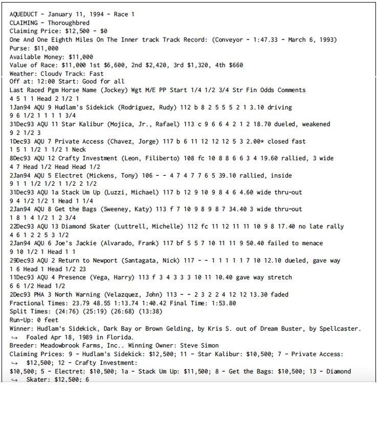
HORSE RACING PREDICTION USING GRAPH-BASED FEATURES

                                    By

                          Mehmet Akif Gulum
                     B.Eng., Erciyes University, 2014

                                  A Thesis
                     Submitted to the Faculty of the
        J. B. School of Engineering at the University of Louisville
                in Partial Fulfillment of the Requirements
                             for the Degree of

                 Master of Science in Computer Science

       Department of Computer Engineering and Computer Science
                       University of Louisville
                        Louisville, Kentucky

                                May 2018
Copyright 2018 by Mehmet Akif Gulum

         All rights reserved
HORSE RACING PREDICTION USING GRAPH-BASED FEATURES

                                By

                      Mehmet Akif Gulum
                 B.Eng., Erciyes University, 2014

                     A Thesis Approved On

                         April 24th , 2018

                              Date

               By the following Thesis Committee:

            Mehmed Kantardzic, Ph.D., Thesis Director

                     Adel Elmaghraby, Ph.D.

                     James E. Lewis, Ph.D.

                                ii
ACKNOWLEDGEMENTS

        I would like to convey my special regards to my distinctive advisor, Dr. Mehmed Kantardzic

for his endless guidance, friendly support and exhilarated encouragements during fulfillment of this

work.

        I would like to thank Dr. Adel Elmaghraby and Dr. James E. Lewis for accepting to serve

in my thesis committee and being a part of this special milestone.

        I address, likewise, my thanks to my colleagues, and Computer Engineering and Computer

Science Department for their support and friendship.

        Finally, I want to convey my most heartfelt thanks to my family for their continuous support

and unconditional love.

                                                 iii
ABSTRACT

             HORSE RACING PREDICTION USING GRAPH-BASED FEATURES

                                        Mehmet Akif Gulum

                                          April 24, 2018

        This thesis presents an applied horse racing prediction using graph-based features on a set

of horse races data. We used artificial neural network and logistic regression models to train then

test to prediction without graph-based features and with graph-based features. This thesis can be

explained in 4 main parts as follows:

  1. Collect data from a horse racing website held from 2015 to 2017

  2. Train data to using predictive models and make a prediction

  3. Create a global directed graph of horses and extract graph-based features (Core Part)

  4. Add graph-based features to basic features and train to using same predictive models and

     check improvements prediction accuracy.

        Two random horses were picked that are in same races from data and tested in systems

for prediction. With graph-based features, prediction of accuracy better than without graph-based

features. Also We tested this system on 2016 and 2017 Kentucky Derby. Even though we did not

predict top three results from 2017 Kentucky Derby, in 2016 Kentucky Derby, we predicted top four

position.

                                                iv
TABLE OF CONTENTS

ACKNOWLEDGEMENTS                                                                                       iii
ABSTRACT                                                                                                iv
LIST OF FIGURES                                                                                        vii

CHAPTER

  1    INTRODUCTION . . . . . . . . . . . . . . . . . . . . . . . . . . . . . . . . . . . .             1

      1.1   Background . . . . . . . . . . . . . . . . . . . . . . . . . . . . . . . . . . . . . .      1

      1.2   Motivation . . . . . . . . . . . . . . . . . . . . . . . . . . . . . . . . . . . . . .      2

      1.3   Scope and Objectives of the Thesis . . . . . . . . . . . . . . . . . . . . . . . . .        2

      1.4   Organization of the Thesis . . . . . . . . . . . . . . . . . . . . . . . . . . . . .        2

  2    LITERATURE REVIEW . . . . . . . . . . . . . . . . . . . . . . . . . . . . . . . .                3

  3    DATA PREPROCESSING . . . . . . . . . . . . . . . . . . . . . . . . . . . . . . .                 8

      3.1   Data Collection . . . . . . . . . . . . . . . . . . . . . . . . . . . . . . . . . . . .     8

            3.1.1   Download PDF files from the website with scripts . . . . . . . . . . . . .          8

      3.2   Data Parsing . . . . . . . . . . . . . . . . . . . . . . . . . . . . . . . . . . . . .     11

      3.3   Data Preprocessing: . . . . . . . . . . . . . . . . . . . . . . . . . . . . . . . . .      16

  4    INTRODUCTION OF GRAPH THEORY                      . . . . . . . . . . . . . . . . . . . . . .   19

      4.1   Labeled Edge Graph . . . . . . . . . . . . . . . . . . . . . . . . . . . . . . . . .       23

      4.2   Multiple Labeled Edge Graph        . . . . . . . . . . . . . . . . . . . . . . . . . . .   23

      4.3   Graph-Based Features . . . . . . . . . . . . . . . . . . . . . . . . . . . . . . . .       24

  5    MACHINE LEARNING MODELS                   . . . . . . . . . . . . . . . . . . . . . . . . . .   28

      5.1   Artificial Neural Networks . . . . . . . . . . . . . . . . . . . . . . . . . . . . . .     28

            5.1.1   Logistic Regression Model . . . . . . . . . . . . . . . . . . . . . . . . . .      30

  6    EXPERIMENTAL RESULTS                . . . . . . . . . . . . . . . . . . . . . . . . . . . . .   33

      6.1   Using Basic Horse Racing Features to Make Prediction . . . . . . . . . . . . .             38

                                                 v
6.2 Using Additional Graph Features to Make Prediction with ANN . . . . . . . . 40
6.3 Using Additional Specific Graph Features to Make Prediction with ANN . . . 41
6.4 Challenge for Kentucky Derby . . . . . . . . . . . . . . . . . . . . . . . . . . . 44
7 CONCLUSIONS AND FUTURE WORK . . . . . . . . . . . . . . . . . . . . . . . 48
7.1 Conclusions . . . . . . . . . . . . . . . . . . . . . . . . . . . . . . . . . . . . . . 48
7.2 Limitations and Future Work . . . . . . . . . . . . . . . . . . . . . . . . . . . . 49
7.2.1 Limitations . . . . . . . . . . . . . . . . . . . . . . . . . . . . . . . . . . 49
7.2.2 Other Machine Learning Algorithms . . . . . . . . . . . . . . . . . . . . 49
7.2.3 Additional Features . . . . . . . . . . . . . . . . . . . . . . . . . . . . . . 49
REFERENCES 50
CURRICULUM VITAE 52
viLIST OF FIGURES
FIGURE Page
1.1 Win, Place, Show - How To Bet On Horses. . . . . . . . . . . . . . . . . . . . . . . . 1
2.1 The S&C Racing System . . . . . . . . . . . . . . . . . . . . . . . . . . . . . . . . . . 4
2.2 The AZGreyhound System . . . . . . . . . . . . . . . . . . . . . . . . . . . . . . . . 5
2.3 Results compared Baseline . . . . . . . . . . . . . . . . . . . . . . . . . . . . . . . . . 6
3.1 Overall Design . . . . . . . . . . . . . . . . . . . . . . . . . . . . . . . . . . . . . . . 8
3.2 Dates of horse Racing . . . . . . . . . . . . . . . . . . . . . . . . . . . . . . . . . . . 9
3.3 Example of one Track . . . . . . . . . . . . . . . . . . . . . . . . . . . . . . . . . . . 9
3.4 Script Code . . . . . . . . . . . . . . . . . . . . . . . . . . . . . . . . . . . . . . . . . 9
3.5 Download the PDF . . . . . . . . . . . . . . . . . . . . . . . . . . . . . . . . . . . . . 10
3.6 Example of captcha . . . . . . . . . . . . . . . . . . . . . . . . . . . . . . . . . . . . 10
3.7 The capthca code . . . . . . . . . . . . . . . . . . . . . . . . . . . . . . . . . . . . . . 10
3.8 Example of Script Results . . . . . . . . . . . . . . . . . . . . . . . . . . . . . . . . . 12
3.9 Example of Pdf File . . . . . . . . . . . . . . . . . . . . . . . . . . . . . . . . . . . . 13
3.10 Text String . . . . . . . . . . . . . . . . . . . . . . . . . . . . . . . . . . . . . . . . . 14
3.11 Sample table . . . . . . . . . . . . . . . . . . . . . . . . . . . . . . . . . . . . . . . . 14
3.12 Log File . . . . . . . . . . . . . . . . . . . . . . . . . . . . . . . . . . . . . . . . . . . 15
3.13 Wager File . . . . . . . . . . . . . . . . . . . . . . . . . . . . . . . . . . . . . . . . . 15
3.14 2017 Result File . . . . . . . . . . . . . . . . . . . . . . . . . . . . . . . . . . . . . . 16
3.15 Distance and Track Type Example . . . . . . . . . . . . . . . . . . . . . . . . . . . . 16
3.16 Example of Distance Type . . . . . . . . . . . . . . . . . . . . . . . . . . . . . . . . . 17
3.17 Track Type in Data . . . . . . . . . . . . . . . . . . . . . . . . . . . . . . . . . . . . 18
3.18 Weather Attributes . . . . . . . . . . . . . . . . . . . . . . . . . . . . . . . . . . . . . 18
3.19 Distance Attributes . . . . . . . . . . . . . . . . . . . . . . . . . . . . . . . . . . . . . 18
4.1 Example of Graph . . . . . . . . . . . . . . . . . . . . . . . . . . . . . . . . . . . . . 19
4.2 Undirected Graph Example . . . . . . . . . . . . . . . . . . . . . . . . . . . . . . . . 20
4.3 Directed Graph Example . . . . . . . . . . . . . . . . . . . . . . . . . . . . . . . . . 20
vii4.4 Adjacent Matrix . . . . . . . . . . . . . . . . . . . . . . . . . . . . . . . . . . . . . . 21
4.5 Model of Horse Graph . . . . . . . . . . . . . . . . . . . . . . . . . . . . . . . . . . . 22
4.6 Adjacent Matrix of Horse Graph . . . . . . . . . . . . . . . . . . . . . . . . . . . . . 22
4.7 Example of Directed Edge Weighted Graph . . . . . . . . . . . . . . . . . . . . . . . 23
4.8 Example of Edge Connected Graph With Specific Conditions . . . . . . . . . . . . . 24
4.9 Example of Edge Connected Graph With Specific Conditions . . . . . . . . . . . . . 24
4.10 Example of Graph for HITS Algorithm . . . . . . . . . . . . . . . . . . . . . . . . . . 26
4.11 Adjacent Matrix for HITS Algorithm . . . . . . . . . . . . . . . . . . . . . . . . . . . 26
4.12 Transpose of Adjacent Matrix for HITS Algorithm . . . . . . . . . . . . . . . . . . . 26
5.1 Example of Neural Network . . . . . . . . . . . . . . . . . . . . . . . . . . . . . . . . 29
5.2 Example of Neural Network . . . . . . . . . . . . . . . . . . . . . . . . . . . . . . . . 30
5.3 Logistic Function . . . . . . . . . . . . . . . . . . . . . . . . . . . . . . . . . . . . . . 31
5.4 Schematic of Logistic Regression . . . . . . . . . . . . . . . . . . . . . . . . . . . . . 31
6.1 Horse Races Features for Some Specific Days . . . . . . . . . . . . . . . . . . . . . . 34
6.2 Comparing Horse Races Results for Some Specific Days . . . . . . . . . . . . . . . . 35
6.3 Example of Horse Race Result in 2017 . . . . . . . . . . . . . . . . . . . . . . . . . . 36
6.4 Features of Two Horses in 2016 and 2017 . . . . . . . . . . . . . . . . . . . . . . . . 37
6.5 Comparing Two Horses Results in 2016 and 2017 . . . . . . . . . . . . . . . . . . . . 37
6.6 Compare Prediction Accuracy With ANN and The Baseline . . . . . . . . . . . . . . 39
6.7 Compare Prediction Accuracy With ANN, LR and The Baseline . . . . . . . . . . . 39
6.8 Compare Prediction Accuracy With Additional Graph features ANN . . . . . . . . 40
6.9 Compare Prediction Accuracy With Additional Graph features ANN and LR . . . . 41
6.10 Compare Prediction Accuracy With Additional Specific Graph features ANN . . . . 42
6.11 Compare Prediction Accuracy With Additional Specific Graph features ANN and LR 43
6.12 2017 Kentucky Derby Horses . . . . . . . . . . . . . . . . . . . . . . . . . . . . . . . 44
6.13 Predictions of Experts . . . . . . . . . . . . . . . . . . . . . . . . . . . . . . . . . . . 45
6.14 Example of Model Prediction . . . . . . . . . . . . . . . . . . . . . . . . . . . . . . . 45
6.15 Comparing Results in Kentucky Derby 2017 . . . . . . . . . . . . . . . . . . . . . . . 46
6.16 Comparing Results in Kentucky Derby 2016 . . . . . . . . . . . . . . . . . . . . . . . 47
viiiCHAPTER 1
INTRODUCTION
1.1 Background
Horse racing is a sport that includes two or more horses ridden by jockeys [1]. Almost every
day of the year, some race occurs all around the world. There are different types of races such as
flat race, which is run over a level track at a preplanned distance; harness race, which usually pulls
a two-wheeled cart for horses. In this thesis, we use flat race for the models.
While horses are sometimes raced only for sport, a majority part of horse racing is relevant
with gambling components [2]. Many people in the world bet horse races and want to earn money.
For example, betting on the Kentucky Derby in 2017 totaled approximately $139.2 million [3]. There
are many betting systems in horse racing but basically called win bet which is guessing the winner
horse in the race. Most traditional bets are usually called straight wagers, are Win, Place Show.
The win is if a person wagers money to a horse, he wins only his horse finishes first; the place is,
he wins if his horse finishes the race first or the second position; the show is, he wins if his horse
finishes the race first, second or third position.
Figure 1.1: Win, Place, Show - How To Bet On Horses.
11.2 Motivation
We choose horse racing data because horse racings contain dozens of variables such as track
type, weather, jockeys to name but a few. These horse race conditions support more challenge for
prediction. Also, horse racing has been a well-known subject in machine learning field, so that we
would like to work horse racing data for prediction.
Horse racing is not the only sport that is researched for data mining applications. There
are different sports data such as tennis, college basketball are using in especially predictive models.
When we finish the model, it may be extended to other applications of data mining in different
sports.
1.3 Scope and Objectives of the Thesis
The main objective of this thesis shows that graph-based data help better prediction of horse
race results. Usually, a prediction model is based on attributes that are from horses and training
based on hundreds of races and are made a prediction [4]. Besides of these set of attributes and this
model, we want to extend set of features which are not directly evaluated from original data, but they
are generated based on the global picture of horse races. For these attributes, we are analyzing the
graph of horses. According to the graph of horses that are created with data, to establish additional
relation which will be extended set of attributes and, with these extended set of attributes and the
basic set of attributes, we are trying to prove prediction will be improved or not.
For prediction part, we will use predictive models for horse racing, based on two machine
learning methodologies that are artificial neural network and logistic regression. One of the biggest
effort was data preparation part because we don’t have available data so, we need to find useful data
and prepare it for using the model.
1.4 Organization of the Thesis
The remainder of this thesis is as follows: Chapter 2 provides a literature review of related
works and applied methodologies. Chapter 3 gives data preparation and feature extraction. Chapter
4 describes applying methodologies and experimental results. Finally, chapter 5 provides conclusion
and future works.
2CHAPTER 2
LITERATURE REVIEW
Before betting a horse racing, people want to analyze some contributions such as horses and
jockeys to find possible winners. There are many newspapers and websites give some tips about win-
ning possibilities, but these possibilities are not very close accurate of predictions. Many researchers
have been studying racing predictions using different several algorithms. In this review, methodolo-
gies researched and applied by different researchers to established models have been investigated.
Williams and Li [5] studied horse racing in Jamaica to the prediction of winners. They used
Artificial Neural Network methodology primarily. In Jamaica, horse races in distances of 1 to 3 km.
Data were collected from 143 races from January to June 2007. They used four different learning
algorithms and their results were compared. They studied different variables to horse racing such as
horse, jockey, past position, track distance and horses finishing time and others as input to Artificial
Neural Network. They used 80% of data for training and 20% of data of testing. Four algorithms
predicted correct horses with an accuracy of around 70% and they took more or less similar results.
Similar to Williams and Li [5] Davoodi and Khanteymoori [4] also used artificial neural
network for prediction system. They investigated horse racing predictions for just one race track
in New York using artificial neural networks. Data were collected from 100 races for analysis from
January 2010. Artificial Neural Networks were used to predict the finishing time of each horse in
a race. They used five supervised algorithms; Gradient Descent BP Algorithm, Gradient Descent
BP with momentum Algorithm, Quasi-Newton BFGS Algorithm, Levenberg-Marquardt Algorithm
and Conjugate Gradient Descent Algorithm in their study to compare performances. Eight features
had been used for input: Horse weight, race type, trainer, jockey, number of horses in a race, track
distance and condition and weather. In network, one neural network is used to represent one horse.
Each neural network has eight inputs and one output that is horse final position time . While BP
and BPM were the best at predicting winners and Levenberg-Marquardt was found to be the fastest
algorithm and all algorithms used had an average accuracy of around 77%.
Pardee [6] also studied artificial neural networks, but he predicted the result of football
3matches in college. A model was developed using past football seasons data and predict the winning
team. He used data for training and testing from 11 games for each team which played in the
seasons of 1998 and 1999. The system predicted which team will win the college football game with
an accuracy of 76%. Besides if given more data about the teams previous performances, the degree
of the accuracy of system could be better.
Robert P. Schumaker [7] used support vector regression to predict horse ranking for next
race. He used a model name was The S&C Racing System shown figure 2.1. This system consists
several major components; data module, the machine learning part, betting engine and evaluation
metrics. He used the traditional betting engine that is Win, Place or Show.
Figure 2.1: The S&C Racing System
Schumaker [7] used several features such as fastest time, win percentage, place percentage
and average finishing position for the last several races. Results were tested three dimensions of
evaluation that are accuracy, payout and efficiency. He was trying to find balance point for accuracy
and payout when payout becomes maximum.
In addition to horse racing data, greyhound racing data are also using for prediction systems
because some conditions are similar to horse racing data. Robert P. Schumaker and James W.
Johnson [8] used support vector regression algorithm on more than 1900 races and 31 different dog
tracks to made prediction. They used an almost similar system from Robert P. Schumaker [7], but
they used different betting engine with the traditional engine in the system name was AZGreyhound
System that shown figure 2.2. In Straight bets, there are exacta, trifecta and superfecta wagers.
While in exacta, the bettor should predict 1st and 2nd place for dogs respectively, in trifecta is more
harder by trying to predict first three places. In Superfecta, the bettor should determine best 4 dogs
will pass finish line. In Box bets, the bettor should try every combination of placement.
In this paper, they tested three dimensions of evaluation; accuracy, payout and efficiency
4Figure 2.2: The AZGreyhound System
and they compared betting engine with .Their system predicted Wins and efficiency around for high
accuracy low payout, and low accuracy high payout with different betting engine. They found that
accuracy and payout are connected.
Hsinchun Chen et al. [9] also investigated prediction with greyhound racing. They tested
artificial neural network algorithms (back propagation) and ID3 with 50 different variables, but they
could not use all of the variables because the neural network didn’t work with them. That’s why
they filtered more important variables and analyzed them. They used around 66% of data for train-
ing and around 33% for testing. Their system was predicted winners on 34 races and no winners
were predicted for 16 races.After that, they placed bets on dogs that were predicted winners by the
system in real. If a dog was predicted to finish first position, they put a $2 wager. ID3 algorithm
was %34 accuracy and $69.20 payout, the neural network had %20 accuracy and a $124.80 payout.
In finally they found that the neural network predictions had better performance instead of human
experts.
Prediction systems are not only for races, but also scientists use several sports. Baulch [10]
tried to predict winners in rugby league and basketball games using artificial neural network. He
focused mainly on the Backpropagation method and the Conjugate Gradient method for training.
He used different type of features such as the teams previous performances, the number of wins and
the average scores per game to predict the winner. His results are an accuracy that lies between %55
and %58.2 for rugby and between %49 and %59 for basketball. Finally, he showed that artificial
neural networks helped a great performance in sports predictions and if research can be extended,
results will be better.
Another example system for prediction horse racing is using Support Vector Machine Re-
5gression [11]. The author used 20 different features and all features had a value of -1,0 or 1. For
example, for the feature of Horse Win%, if horse’s win percentage is more than %50 ”1” else ”0”
and with this training, he tried to predict approximative finishing line position for horses. Data
was prepared from December 2016 to February 2017 for training and March 2017 for testing. He
tried to compare his result with the baseline (the morning line). The baseline is a list of entries
for a horse race with the probable betting odds as estimated by a track handicapper issued before
wagering begins. In results, he tried different strategies.Generally, He picked horses that have the
better winning chance from morning line. In totally around 2900 races, for morning line(the base-
line), the percentage of the favorite horse was %26 and its win place show results were around %58.
For his model, favorite horse winning percentage was %28 and came in 1st 2nd and 3rd 1820 times
%63. He also used different type of techniques and he found that machine learning works better
than baseline.
Figure 2.3: Results compared Baseline
In our thesis one of the big effort is creating a graph and extracting features from this global
graph. Suvrat Bhooshan, et al. [12] investigated the application of network analysis for prediction.
They used data from Major League Baseball (MLB) and the National Football League (NFL).
They created directed graph as a relationship between teams for each league and it is the win-
loss relationship for every two teams.They calculated the weight of edges between two teams; (the
number of times team i won against j - the number of times i lost against j). For positive weighted
on (i,j) means j is better than i, and negative is the exact opposite.
They used a ranking algorithm explained by Guo et al. [13], and they ordered nodes of
subgraphs. That means higher ranked nodes have more incoming edges than outgoing edges.After
this operation, they split nodes into two groups names were leaders and followers and they repeated
these process until reached for global order. Furthermore, they applied two methods. One of them
6is weight difference for a node that is;
X X
dw (i) = w(i, j) − w(j, i)
(i,j)∈E (j,i)∈E
w(i,j) is weight of (i,j). Another algorithm is HITS algorithm that is a link analysis algorithm,
rates Web pages, nodes for graphs. Hits algorithm has two different scores but, they just used
authority score, not hubs score for each node as a ranking. Accurate classifier were improved with
these rankings. They also used triads features similar to Jure Leskovec et al. [14]. Triad consists
of three nodes and the possible connections between them. For example, if a connection between u
and v nodes also can include another node that is w. Normally when we look two pairs of nodes
(u.v) edges and, we can just see two different values that one of them is positive and other value is
negative. In the triad, we can see four different values between u to v that are (++,+-,-+,–) from u
to v. They used this triad between all pairs of nodes for taking values (scores) not directly connected
between two pairs of nodes, but also undirected connections They used logistic regression algorithm
for prediction In final, When they compared results, They found that accuracies NFL better than
accuracies of MLB. Also when they compared expert ranking system (the baseline) they said that
their system was more objective because expert systems handled recent games, not the entire season.
7CHAPTER 3
DATA PREPROCESSING
In this chapter, we will present data preprocessing for model. Data preprocessing is a
technique that is converting raw data into a clear format [15] . In the real world, data usually
contain many errors or incomplete. Data preprocessing helps to resolve these issues prepare horse
race data for analyzing. In this thesis, data preprocessing part design will be like in figure 3.1.
Firstly we will show data collection from specific website that name is equibase [16]. After that, we
will show data preparation part as Sethabhisha Naidu Nerusu et. al. [17]
Figure 3.1: Overall Design
We will download pdfs files from website. After that we will design a program to convert
the pdf to the markup text annotates text [18], and then to parse the markup text into C# objects.
Finally we will convert horse race data to CSV files.
3.1 Data Collection
Data collection part can be explained two main parts as follow :
1. Determine data from Equibase horse racing website held from 2015 to 2017 and downloading
the daily race forms from Equibase website with semi-automated scripts.
2. Collect the pdfs downloaded put data in a tab delimited text file
3.1.1 Download PDF files from the website with scripts
The goal of the scripts is to get all the race/track information from 2015 to 2017 as PDF files.
In the website, race records are as pdf files and these pdf files don’t only consist one race, but also
include several races because website minimizes number of requests. In one day, there are several
8Figure 3.2: Dates of horse Racing Figure 3.3: Example of one Track
tracks using for horse racing, so we will try to download each track from each day. Strategy is for
each date, load the web page listing all the tracks where races happen and each track load the results
for all races of the day. There are no races some days or some tracks, so we should eliminate them
because system does not eliminate these empty files and it will bring them also like there are races in
those days or tracks. If we also add these empty days or tracks, it is possible to receive errors during
the parsing part. We will use equibase website for collecting data (http://www.equibase.com/).
When we opened website/historical part, we can see that dates for horse racing like figure 3.2.
When we clicked one of the days, we can see tracks that there are races in that day and each
track has raced as figure 3.3.
We use HTML code to frame the URLs automatically for all tracks in a day. It contains
the list of all the tracks codes in the tid=xxx form. We will use them to find the tracking code.
We tried to get the list of the tracks with bash code. We will use curl to get the HTML from the
website, grep isolates the href lines and sed processed the href and extracts the tracking code figure
3.4, figure 3.5. We cannot call script directly because it is called by the download-pdfs script. If
you call it directly, the syntax is ($ ./get-available-tracks 2016 1 1) and output is as such as AQU,
CMR, DED, FG, GG,GP.
Figure 3.4: Script Code
With these scripts, we extract pdf files that contains more things. The PDF contents is
returned by the web-site and saved to a pdf file. When we try to download pdf files, we have big
9Figure 3.5: Download the PDF
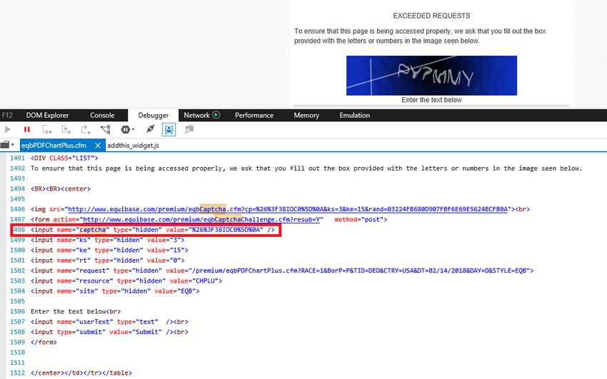
problems that is captcha. A captcha is a security for websites use to avoid robots to browse the site.
It sends back a scrambled image to the user for proving user is human or not.
Figure 3.6: Example of captcha in Equibase website
Equibase website sends captcha every ten requests. If we don’t defeat it, we cannot download
data automatically. And also we should know how it works because it can be changeable every
captcha. We used internet explorer debug mode and we can check every HTML code and every
element on the page where we try to defeat captcha.
Figure 3.7: The capthca code
The web page includes a hidden captcha code, which contains a version of the captcha text.
For the system that is created, we don’t need to look encryption part we just have to send back
the captcha text along with the captcha code. Actually, there is 2 type of captchas in the website;
10protecting the tracks list and protecting the pdfs. We need to enter the captcha text and activate
the Net tab than The Net tab contains a POST statement, which is the captcha send the website.
There is a really important command that name is captcha-get-available-tracks is stored. We need
to send the script before every get-available-tracks command because it generated a script and this
script resets the allowed every 10 requests.
We have 4 different scripts captcha-get-available-tracks, get-available-tracks: called the
captcha-get-available-tracks and get track list, captcha-download-pdfs send reset request for pdf
and download-pdfs. When we run scripts, we should use like:
./generate-dates end-year end-month end-day start-year start-month start-day
so, until which date we want to download is beginning and from which date we want to start
is final
$ ./generate-dates 2017 1 12 2017 1 1
And results are;
./download-pdfs 2017 1 12 17 01 10
./download-pdfs 2017 1 11 17 01 09
./download-pdfs 2017 1 10 17 01 08
./download-pdfs 2017 1 9 17 01 07
./download-pdfs 2017 1 8 17 01 06
./download-pdfs 2017 1 7 17 01 05
./download-pdfs 2017 1 6 17 01 04
./download-pdfs 2017 1 5 17 01 03
./download-pdfs 2017 1 4 17 01 02
This scripts will run for everyday and generates results. For example in above we can see
that download races from 2017/1/12 to 2017/1/1. In final we took following results (figure 3.8) that
displays date and track name (AQU is Aqueduct);
Scripts didn’t always work sometimes we got some errors and when we took this error we
regenerated manually. Also rarely, some pdfs files downloaded as HTML file so, sometimes we need
to download them manually.
3.2 Data Parsing
A PDF Parser is a software which you can use to extract data from PDF documents. There
are many different document types you can extract data PDF files such as text paragraphs, single
11Figure 3.8: Example of Script Results
data fields, tables and lists and images. If a pdf file contained image, we need to use optical character
recognition to extract these images from pdf files. Horse race data doesn’t include images figure 3.9
so, we don’t need to use OCR system.
We need to extract horse race data from pdf files automatically like project [17] We don’t
need to write hundreds line of codes. We will use the iTextSharp framework and C#. Important
part for parsing is a strategy to reliably and correctly parse the data because parser give us which
texts are in pdf file but, we should find exact location of texts that we want to extract.When we
process this PDF document with iTextSharp with we end up with the following text string in figure
3.10.
In this figure, the first line includes track, date, and race number. Other lines contain the
race and horse types, layout becomes more variable so, text position becomes less reliable, except
when we can find a beacon to fix on and start counting rows again. We will use text label technique
that allows us reliable and more data.It looks like a key that helps find data quickly.
In the basic parsing, some data are created in a superscript font and there are three tables
in the PDF page that can have a variable number of rows and columns. It is not enough to identify
all parts of a document with raw text so, we need to find a mechanism that is reliable and we need
to find way to provide the parser with hints. We used two kinds of markup tags to help to parse the
PDF.
Superscripts: Some parts of text are surrounded by superscript text. For example, text
like 4 AQU 5 output text is < 4 > AQU < 5 > so, superscript text is really easy to find.
Tables: When we look tables that we want to parse, we can see that we should make clear
12Figure 3.9: Example of Pdf File
such as table’s start and end etc.
When the text is completely marked up, we are ready to convert the pdf to the text and to
parse the markup text into C# objects.
The data goes to PDF file than markup language defined earlier in the document than C#
representation of the race objects. This is an in-memory data model which will be transformed into
the final format. In final, we are trying to convert data into a CSV file through a CSV renderer
figure 3.11.
The markup generation is class HorizontalTextExtractionStrategy, derived from the iTextSharp
class LocationTextExtractionStrategy. The main function of this class is, it is invoked by the
iTextSharp parser for every single word of the document. The parameters of this function con-
tain the word,data position and format. The function can determine if a new line starts.
We need to take a lot of data information and should modify each word on the fly we will
use a filter chain. Each word makes its way through the filter in filter chain and the output of the
13Figure 3.10: Text String
Figure 3.11: Sample table
first filter is fed into the second filter. Each filter has opportunities the following:
1. Change the word that transmits like parameter before you passed the next filter
2. Bypass subsequent filters and ignore the word. After that, word that is ignored will not
be in the markup text. Every word is passed into the filter chain.
Every filters take one word so, text passed through a pre-processor chain, in fact, to make
calculation again or pattern recognition and after that, it goes preprocessing. Similarly, the markup
text is passed through a post-processing chain to prepare the final result. Some filters connect with
14some other filter status and all filters communicate with each other via publication and subscription.
Usually one filter in the chain has already finished its job than other filter will be active. If we do
not do this, a filter can be confused if a horse name contains the word. That is one of the errors
we faced. The markup text is converted to C# objects, and These objects are defined in the
Model subdirectory. While the C# object hierarchy cannot render CSV file, the C# objects are
de-normalized will be written as a CSV file in different objects.
The program interface is easy: EquibaseParser.exe input1 input2 input3 ...inputn and output
has three files are created as a result.
Figure 3.12: Log File
Log File has the log of all the races processed. If any file stopped in error we can see in log
file and we can fix error that occurred while running
Figure 3.13: Wager File
Wager File includes especially standard wager types other attributes such as track name,
date and payoff for horse races (figure 3.13).
15Figure 3.14: 2017 Result File
Result File is actual data and attributes such as weather, track name, date, distance and
track type that we use in model shown in figure 3.14.
3.3 Data Preprocessing:
In horse racing distance of track and track type are important attributes that are affect horse
racing results. In the data, these attributes are together like one attribute as shown in figure 3.15.
Figure 3.15: Distance and Track Type Example
We should split distance and type of track into 2 attributes. For example One Mile and
Seventy Yards as a distance and Dirt as a track type. We should split 2 different attributes because
there is no connection with these attributes for all of races.
16Figure 3.16: Example of Distance Type
On the other hand, distance section is in words and in different units like yards, miles, and
furlongs. So, we should convert all type of distance to one type as a mile. Also, we should converted
words to numeric values manually like figure 3.16.
When we started to search horse races, we saw that there are a lot of conditions and attributes
affect results but, some of them are important because of they affect directly results. Like most of the
research and paper, Elnaz Davoodi et al [4], they used as features horse weight, type of race, horse’s
trainer, horse jockey, number of horses in the race, race distance, track condition and weather. When
we analyzed other research and races, we can see that jockey is more effective than trainer in races.
Also horse race data just include same type of races. track type weather, horse weight, number
of horses in one race are important conditions and attributes in horses races. With all of these
researches and horse races results we decided to use 8 different features for horse racing prediction:
track type, weather , jockey , horse’s past final position, horse weight, number of horses in the race,
track condition and distance and also for comparing we will use probable betting odds (the baseline)
attributes. Before input data for training and testing we should change some of them nominal to
numeric. Horse’ weight, number of horse, past position and distance are numeric values. For track
type, weather and track condition, we encode them into numerical values for using as input data.
For horse jockey values is calculated by dividing the number of wins by the number of rides in horse
racing data. Some of the attributes in data are below figures.
17Figure 3.17: Track Type in Data
In figure 3.17, we can see that track types such as dirt, turf and inner. Dirt type is more
than other type in horse races.
Figure 3.18: Weather Attributes
in figure 3.18 we can see weather conditions in horse races. In data, most of the races are
organized in clear and cloudy weather
Figure 3.19: Distance Attributes
In figure 3.19, we can see that distances in data. Minimum distance in one race is 0.056 mile
and maximum distance in one race is 2.25.
18CHAPTER 4
INTRODUCTION OF GRAPH THEORY
The graph is basically a network that defines the relationship between points [19]. Each
object in a graph is called a node. Objects in a graph are described by nodes, and relations between
these objects are described by graph edges [20].
If we want to understand system that is really complicated, we need to know how its elements
interact with each other. In other words, we need a map of its global picture.
Figure 4.1: Example of Graph
In figure 4.1, we can see a network of graph. In this network, components (computers) often
called nodes or vertices and the interactions between them, called links or edges. With this graph
network, we can see whole system of computer network and connections like a big picture.
It is possible to divide graphs as directed graphs and non-directed graphs, depending on
whether the edge types [21]. If the set of edges are unordered, this graph called undirected graph
and if a graph consists of vertices and ordered pairs of edges, this graph called directed graph [22].
19Undirected Graph
Undirected graph is a graph that has relations between pairs of nodes, so that each edge has
no directional character [23].
Figure 4.2: Undirected Graph Example
For example,in figure 4.2 a undirected graph shows consisting of 4 nodes and 4 edges. This
graph can be expressed as G = ([A,B,C,D] , [(A,B),(A,C),(C,D),(A,D)]) . Therefore, graphs are
written in the form of G = (V, E), ie, nodes and edges.
Directed Graph
Unlike undirected graph, directed graph set of nodes are connected pairwise by directed
edges [24] so, we can say that each edges like one way streets.
Figure 4.3: Directed Graph Example
In figure 4.3, There is a directed graph. Arc is directed edge way from a node to another
node. Sometimes some nodes has edges for themselves (loop edge). if one node has two edges to
20other node it called multiple arc or multiple edges.
Labeled Graph
In graph, nodes have some degrees. Degree is number of edges incident on a node and two
type of degree a node can has [25]. In-degree is number of edges entering and out-degree is number
of edges leaving. For example graph that is above, node three (Node3) has 1 out-degree and 4
in-degree and total degree is 5.
Adjacency Matrix
Graphs also represent as a matrix that is called adjacent in graph theroy and computer
science. Adjacent matrix show pairs of vertices connect in a finite graph or not [26].
Figure 4.4: Adjacent Matrix
In graph and matrix in figure 4.4, we can see that connections represent 0 and 1. For
example node 6 has one connection with node 4 so, other numbers are 0 and with node 4 value is
1 in diagonal. Also node 5 has 3 connections and it has three 1 value that are with node 1, node 2
21and node 4. This graph is also example of non-labeled graph
We can used graphs in data organization, computational devices as well as many types of
processes in physical, biological, social fields and especially network systems as a model [27]. We can
see graphs in everywhere in the world. Even if friendship with other people is a graph network. [28]
In this thesis, we want to create a global picture of horse races with directed graph and
extract some additional features that generated connection horses from a directed graph as well as
basic features that are directly come from horse races data. Important part that, we want to create
two type of graph for new features. One of them includes only basic edge labeled connections between
horses and other describes graph contains edge labeled connections that include some conditions.
We will use similar approaches as Suvrat Bhooshan et al. [12] for this models.
Figure 4.5: Model of Horse Graph
Figure 4.6: Adjacent Matrix of Horse Graph
For example in graph and adjacent matrix in figure 4.5 and 4.6, if we look H4, it has 2
out-degree and 2 in-degree. Out-degree represents win edges and in-degree represents lose edges. In
this thesis, two kind of graphs are created: labeled edge graph and multiple labeled edge graph.
224.1 Labeled Edge Graph
For basic edge labeled graph model, we want to use the win-loss spread [29] of horses for all
races in the data. Each horse has a relationship with other horses as weighted in edges. For example
if a horse i beat another horse j, we will put an edge from horse i to horse j, or in a race, if a horse
loses to another horse, we will put an edge from winner horse to other horse. Then, we will calculate
win-loss spread between horse i and horse j as a weighted edge (i,j). For instance, if a horse i beat
3 times other horse j we will put 3 edges from horse i to horse j and horse j beat 2 times horse i we
will put 2 directed edges from j to i. Then we will calculate these edges (3 − 2 = 1) and we can say
edge weight is 1 from i to j. One of example is in figure 4.7
Figure 4.7: Example of Directed Edge Weighted Graph
4.2 Multiple Labeled Edge Graph
Other type of graph is same the system as basic edge labeled graph but, we added some
conditions on edges such as weather, track condition or track type. For example, when we want
to predict a horse racing in some specific conditions such as cloudy weather and muddy track, we
can directly extract features from graph that contains these conditions in edges and we can find
more specific results. For example we take 2 horses and we want to know which will beat other
horse in sunny weather and Dirt track. After creating the graph with weighted edges and these
two conditions on edges, we will eliminate other edges that include different conditions and we will
extract features from this edge labeled graph with specific conditions. In figure 4.2 and 4.3 show
that an example of specific edge graph. Different colors include same type of conditions and we just
look one type of color that is same conditions we have determined.
23Figure 4.8: Example of Edge Connected Graph With Specific Conditions
For Example in figure 4.8, we can see that some edges have two conditions that distance 1
mile and dirt track type and other edges contain different conditions that are distance 0.75 and turf
track type.
With these conditions, we eliminated other connections like figure 4.9 and we created the
graph specifically with these conditions. These conditions are not only distance and track type, we
can decide when we picked two pairs of horses and we can change with different mutual conditions.
Figure 4.9: Example of Edge Connected Graph With Specific Conditions
4.3 Graph-Based Features
When we create a system, we need to extract some features or values from the system, and
we can use them in different scientific fields such as machine learning and statistics. The graph
is a big global system. That is why we need to extract some features to use approaches. Feature
extraction covers narrowing resources to describe a large set of data [30]. When we are performing
analysis of a system or graph, important problem is number of variables. Analyzing large data or
system requires a lot of memories. That is why we need to construct combinations of the variables.
Important part of the feature extraction is determine which features you use [31].
24After creating the graph, we need to find which features we can use and how to extract
features from the graph. In Guo et al. [13] investigated an algorithm that ordered the nodes by
the degree difference. They used how many edges coming from other nodes to node i minus how
many edges going from nodes i d∆ = din − dout and if a node has higher ranked it should have
more incoming edges than outgoing edges. After this ranked score, they used a parameter α and
separated into two class of nodes that are leaders Vl and followers Vf . Than they repeated same
processes and until global achieved.
In this thesis, we will use similar ranking score but we also need to give averages because
some horses have more than races than others so, if we give directly incoming edges minus outgoing
edges it can be a problem. For example, a horse has 3 races and 3 times win. Other horses has
9 races and 6 times win 3 times lose. If we directly calculate d∆ = din − dout it will be not equal
din −dout
system. That is why we made d∆ = n , n is number races that attend a race.
Suvrat Bhooshan et al. [12] also investigated for a node i edge weight difference as
X X
dw (i) = w(i, j) − w(j, i)
(i,j)∈E (j,i)∈E
We will also use the same approach as a graph feature in the graph.
There is another algorithm that can be useful and improve nodes ranking score is HITS
algorithm. The HITS algorithm that is Hyperlink-Induced Topic Search (HITS) is an analyze
algorithm for links of networks that rates Web pages, nodes in graphs etc. [32]. The HITS algorithm
computes two numbers for a node. Authorities calculate the node value based on the incoming
edges. Hubs calculates the node value based on outgoing edges. For example there is a graph and
three node that are X, Y and Z figure 4.10.
25Figure 4.10: Example of Graph for HITS Algorithm
The adjacency matrix of the graph is in figure 4.11;
Figure 4.11: Adjacent Matrix for HITS Algorithm
After compute adjacent matrix we will compute transpose of matrix in figure 4.12;
Figure 4.12: Transpose of Adjacent Matrix for HITS Algorithm
1
If hub weight vector is accept in the beginning like:
1
1
We compute the authority weight, matrix transpose * hub weight vector;
26
0 0 0 1 0
∗ 1 = 0
0 0 0
1 1 0 1 2
And after that we update the hub weight matrix * authority weight ;
0 0 1 0 2
∗ 0 = 2
0 0 1
0 0 0 2 0
When we look these two matrix we reached that node X and Z is a hub since it has 2 hub
score and node Y is the most authoritative since it has 2 authority score. In Suvrat Bhooshan et
al. [12], they applied HITS algorithm just only hubs score for each node as a ranking. We will use
also similar algorithm for the graph to improve ranking score’s quality.
When we extracted graph features, we faced a problem that is about undirected edge scores.
In the graph model, we just have directed edge features. Similar to Jure et al. [14] we also will use
triad features for the graph. For example, the features between node u and node v would also be
calculated with another node w that is between (u,v).
(sign(u, w), sign(w, v))∀w∈V :(u,w)∈E,(w,v)∈E
For example, in two nodes (u.v) if we look directed edges, we just can see two different values
that are win or lose from u to v but, when we look undirected connection between u to v, we will
add also w node. Moreover, with this connection, we have four different values from u to v that are
u beat w w beat v, u beat w w lose v, u lose w w beat v and u lose w w lose v. We will use this
triad methods for all pairs of horses and took values for undirected edge scores.
In conclusion, we will use edge weight score , node score and triad feature as graph features
in the graph and also we will use HITS algorithm for improving quality of features. We will use
these features becasue we wanted to use directly relationship with horses. Basic features are coming
from directly horse racing data so, there is no relationship between horses in horse race data but,
in the graph, features are extracting from big picture of horses and there are connections between
each horses at least in one or two races. That is why we are using graph features and we will use
these features to check improvements of prediction.
27CHAPTER 5
MACHINE LEARNING MODELS
Machine learning is one of the important areas of Artificial Intelligence that researches
algorithms [33] . There are many machine learning methods that can be used for prediction but,
in this thesis, we will use two machine learning models for prediction: artificial neural network and
logistic regression models. There are many researchers that have published models are using logistic
regression. For example, Clarke and Dyte [34] applied a logistic regression model to the difference
in the rating points of the two players for predicting the results. Logistic regression uses to predict
an outcome feature that is categorical form predictor features that are continuous and categorical.
Also a logistic regression model took at seconds in maximum to train. Also we chose the artificial
neural network because ANN model development is highly experimental, and the selection of the
hyper-parameters of the model usually requires a tests and error approach. Moreover, most of the
researchers used the artificial neural network and logistic regression methods for prediction. Also
artificial neural networks can discover complex relationships between the various features in races
or matches. The ANN can give more challenge instead of logistic regression because when we search
it, it takes more time and also the model configuration is more difficult than logistic regression, that
is why we chose these two models and will try to compare results.
5.1 Artificial Neural Networks
An artificial neuron network (ANN) is a system based on the interconnected neurons from
biological neural networks [35]. Each neuron or it is called nodes, calculates a value from its inputs.
Artificial neural networks are typically designed with several layers and each neuron that is in non-
input layer are connected all other neurons. Each connection in the network is a weight and neurons
uses its inputs and their weights to calculate an output value. In figure 5.1, we can see that four
input data come for neural network and processed.
We should train input data before analyzing or testing [35] because neural networks are
trained presenting samples to the network again and again.The general architecture of the network
28Figure 5.1: Example of Neural Network
is that of a multilayer perceptron (MLP), a feedforward network trained by backpropagation. Each
sample contains input data that we put for set conditions and output data that resulting prediction
or answer. The network learns each sample and computes the output using input that we provided.
If there is an imbalance between network output and actual output,the network corrects itself via
exchange its internal connections. This loop process continues until network reached accuracy that
we specified. After neural network is trained, it starts to check similarities between new input data
and give the result a predicted output data.
In this thesis, following system for artificial neural network is used in figure 5.2: In 2015-2016
years data, we will take two horses with 8 different features in a race and we will put network system
for training and we will repeat it until it becomes global achieved. After that, we will pick another
two horses and we will train network repeatedly. For the end, we will have trained each horse with
all other horses in the network.
29Figure 5.2: Example of Neural Network System
After training part, we will use 2017 data for testing. We will pick 2 horses in same race and
we will put these 2 horses and their features in trained network and make a prediction of accuracy
compared real race in 2017.
5.1.1 Logistic Regression Model
Logistic regression is a classification algorithm which uses the calculated logits (score ) to
predict the target class [36]. It transforms its output to return a prediction value which can then be
mapped to two or more discrete classes [36]. Generally, when we create a machine learning program,
we are trying to arrive a prediction for future inputs based on the experience with using the past
inputs and outputs. The logistic function σ(t) is defined as:
1
σ(t) =
1 + e−t
30Figure 5.3: Logistic Function
A logistic regression model for race prediction consists of a vector of n race features [36]
x = (x1 , x2 , x3 ..xn ) and a vector of n + 1 real-valued model parameters β = (β0 , β1 , ...βn ) so for
prediction, they design a point in n-dimensional feature space to a real number then they match z
to a value in the admissible range of probability (0 to 1) using the logistic function.
z = (β0 , β1 x1 , β2 x1 2...βn xn )
Figure 5.4: Schematic of Logistic Regression
Model occurs of optimizing the parameters β the model gives the best results of outcomes
for the training data [36] . In logistic regression, we will use stochastic gradient descent method that
is simple but very efficient approach to discriminative learning of linear classifiers and fit for large
31datasets, updates parameters in every iteration to minimize the error of a model on training data.
This optimization algorithm works like in [37];
-Each training sample is shown to the model one at a time than the model makes a prediction
for a training sample
-Model is updated with errors
- Errors are considered for reducing next prediction.
32CHAPTER 6
EXPERIMENTAL RESULTS
In experimental results, our goal is to extend basic features with graph-based features, train
and test with artificial neural network and logistic regression and compare their results of accuracy
between each other. We will compare artificial neural network and logistic regression with basic
features, the artificial neural network and logistic regression with additional edge labeled graph-
based features, the artificial neural network and logistic regression with additional multiple edge
labeled graph-based features, the baseline that is probable betting odds as estimated by a bookmaker
and also with previous work that is Elnaz Davoodi et. al [4]. Our hypothesis is to try to obtain
better results with additional graph-based based features. In experimental part, firstly we will look
some specific dates and compare the results, after that we will compare results of accuracy for each
methods and previous works and finally we will try our model in real race that is Kentucky Derby.
When we prepared our model, we need to compare some works and show our improvements.
In every race, the bookers or betting operators displayed some values that which horses are most
favorite and which horses are less favorite. We tried to compare morning line (baseline) that is in our
data, and compare horse’s winning probabilities with our model. Also we will compare our results
with previous works.
In horse racing, it is difficult to find 2 horses in same race in same year. It was one of the
big effort to find 2 horses in same race and these horses should be trained from 2015-2016 years
data. Firstly, we used 8 basic features that are directly from horse racing data and implemented
artificial neural network and logistic regression. After trained our 2015-2016 years data, we selected
in 2017 data with each time 2 horses randomly in same race, compared accuracy results with horse’s
winning probabilities.
Our important target is, using additional graph features with basic features, make prediction
and we want to improve our accuracy of prediction. While our basic features are coming directly
from horse racing data, our graph features come a big global picture of horse racing graph. Before
we look accuracy of prediction, we will look some specific dates and races and we will show results.
33Figure 6.1: Horse Races Features for Some Specific Days
We can see in the figure 6.1; we picked randomly two pairs of horses in the same race in
2017 data in different dates. For example first two horses raced in Mahoning Valley Race Course
in March Seventh 2017 and in dirt track, showery weather, with 8 horses, and 1-mile sloppy track.
First horse that name is Majestic Contender ’s weight is 126lb, jockey name is Bryan Metz, final
position in previous race is 3, second horse that name is Bobbys Approval’s weight is 120lb, jockey
name is Bobby R. Rankin and final position in previous race is 4. We compared these horses because
they were in same races in 2017 data and also 2015 2016 data. When we wanted to test these two
pairs of horses, we compared their baseline values that are probable betting odds with our methods.
34Figure 6.2: Comparing Horse Races Results for Some Specific Days
In figure 6.2, we can see results of the baseline, actual races, the ANN with basic features,
logistic regression with basic features, the ANN with graph features, logistic regression with graph
features, the ANN with specific graph features and logistic regression with specific graph features.
Specific graph features mean for instance, when we looked first two horses previous races and their
2017 races, we saw that they raced same distance (1 mile) and same track type (dirt) so, we added
these two conditions in graph edges. We eliminated other edges that are include different conditions
in edges about track type and distance. After that we extracted features from these specific graph
and. In the baseline, if a horse has lower rate, this mean have a higher winning rate. For example
if a horse has 1 odds and other horses has 2 odds, it means first horse winning probability is higher
35You can also read