Anomaly detection from server log data - A case study - VTT
←
→
Page content transcription
If your browser does not render page correctly, please read the page content below
VTT CREATES BUSINESS FROM TECHNOLOGY
Technology and market foresight • Strategic research • Product and service development • IPR and licensing
 • Assessments, testing, inspection, certification • Technology and innovation management • Technology partnership
                                                                                                                                                                                                                   VTT RESEARCH NOTES 2480

                                                                                                                     • • •  VTT RESEARCH NOTES 2480
                                                                                                                     Anomaly detection from server log data: A case study
                                                                                                                                                                            Sami Nousiainen, Jorma Kilpi, Paula Silvonen & Mikko Hiirsalmi

                                                                                                                                                                            Anomaly detection from server log
                                                                                                                                                                            data
                                                                                                                                                                                A case study

ISBN 978-951-38-7289-2 (URL: http://www.vtt.fi/publications/index.jsp)
ISSN 1455-0873 (URL: http://www.vtt.fi/publications/index.jsp)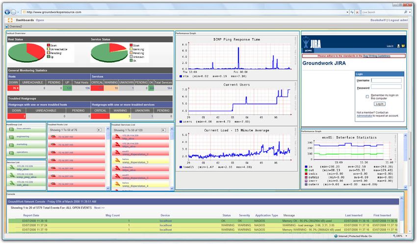

VTT TIEDOTTEITA – RESEARCH NOTES 2480

Anomaly detection from
   server log data
          A case study

     Sami Nousiainen, Jorma Kilpi,
    Paula Silvonen & Mikko Hiirsalmi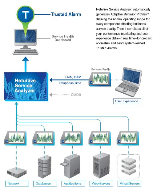
ISBN 978-951-38-7289-2 (URL: http://www.vtt.fi/publications/index.jsp)
ISSN 1455-0865 (URL: http://www.vtt.fi/publications/index.jsp)
Copyright © VTT 2009

JULKAISIJA – UTGIVARE – PUBLISHER

VTT, Vuorimiehentie 5, PL 1000, 02044 VTT
puh. vaihde 020 722 111, faksi 020 722 7001

VTT, Bergsmansvägen 5, PB 1000, 02044 VTT
tel. växel 020 722 111, fax 020 722 7001

VTT Technical Research Centre of Finland, Vuorimiehentie 5, P.O. Box 1000, FI-02044 VTT, Finland
phone internat. +358 20 722 111, fax +358 20 722 7001

Technical editing Leena Ukskoski

                                                    2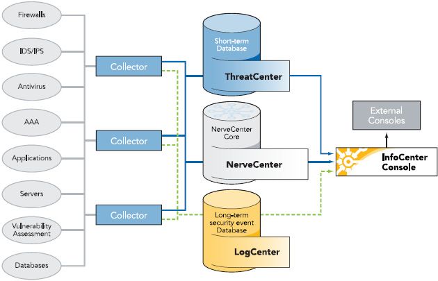
Sami Nousiainen, Jorma Kilpi, Paula Silvonen & Mikko Hiirsalmi. Anomaly detection from server log data.
A case study. Espoo 2009. VTT Tiedotteita – Research Notes 2480. 39 p. + app. 1 p.

Keywords       anomaly detection, data mining, machine learning, SOM, self-organizing map, IT monitoring,
               server log file, CPU, memory, process

Abstract
This study focuses on the analysis of server log data and the detection and potential
prediction of anomalies related to the monitored servers. The issue is relevant in many
mission-critical systems consisting of multiple servers. There it is favourable to be able
detect and even foresee problems to be able to react promptly and apply required
corrections to the system.
  In this study, we have done off-line analyses based on pre-recorded data. In reality, if
the objective is to come up with solutions for detecting anomalies in real-time,
additional requirements and constraints would be imposed on the algorithms to be used.
For example, in on-line situation, higher requirements on the performance of the
algorithm and on the amount of historical data available for the algorithm would exist.
However, we do not address those issues in this preliminary study.
  In addition to the analysis of real data, we have interviewed experts that are working
on the server-related issues on a daily basis. Based on those discussions, we have tried
to formulate practical cases, for which some algorithms and tools could provide
practical utility.

                                                   3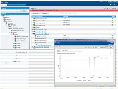
Contents

Abstract........................................................................................................................... 3

1. Introduction ............................................................................................................... 6

2. Background and state-of-the-art ............................................................................... 8
     2.1      Methodologies used in published studies ................................................................................... 8
              2.1.1   Conclusions................................................................................................................ 10
     2.2      Existing software....................................................................................................................... 10
              2.2.1     Nagios (http://www.nagios.org/) ................................................................................. 10
              2.2.2     GroundWork Monitor (http://www.groundworkopensource.com/) ............................... 11
              2.2.3     BMC Performance Manager....................................................................................... 12
              2.2.4     HP GlancePlus ........................................................................................................... 13
              2.2.5     Netuitive Service Analyzer ......................................................................................... 14
              2.2.6     OpenService InfoCenter (NerveCenter) ..................................................................... 15
              2.2.7     Conclusions................................................................................................................ 16

3. Observations from data – explorative approach ........................................................ 18
     3.1      Differences in indicator types .................................................................................................... 18
     3.2      Correlations between indicators................................................................................................ 20
     3.3      Seasonality ............................................................................................................................... 21
     3.4      Anomaly or a consequence of one?.......................................................................................... 23
     3.5      Localization of the problem ....................................................................................................... 24
     3.6      Changes in the state of the system........................................................................................... 25

4. Analysis methods and examples............................................................................. 28
     4.1      Anomaly detection based on SOM analysis.............................................................................. 28

5. Example use cases ................................................................................................. 35
     5.1      Identification of need for updates and verification of their impact.............................................. 35
     5.2      Introduction of a new application............................................................................................... 35
     5.3      Indication of the normal situation .............................................................................................. 36
     5.4      Trend detection ......................................................................................................................... 36

                                                                           4
6. Conclusions, ideas and challenges......................................................................... 37
References ................................................................................................................... 39
Appendices
Appendix A: Explanations for some of the anomalies detected by the SOM method
51. Introduction
1. Introduction
This study focuses on the analysis of server log data and the detection and potential
prediction of anomalies related to the monitored servers. The issue is relevant in many
mission-critical systems consisting of multiple servers. There it is favourable to be able
detect and even foresee problems to be able to react promptly and apply required
corrections to the system.
We have had at our disposal log data recorded from real operating servers. The data
contains various attributes related to the utilization of CPU cores, memory, disks and
filesystem as well as processes. Concrete examples of the attributes analysed include
CPU utilization, amount of free memory and number of processes.
The attributes or indicator values are stored with certain time intervals, e.g., 1 minute
intervals. This might limit in some cases the ability to detect rapid phenomena or
anomalies, since they might get hidden due to the averaging of the indicator values over
the time interval.
The anomalies occurring in the system could be due to several different reasons
including:
• software failures (programming bugs)
• hardware (e.g., some piece of hardware simply breaks down)
• offered load (an exceptionally high load is offered to the system)
• human errors (e.g., configuration errors).
Some indicator values can measure directly a property that we are interested in. For
example, disks have certain capacity and the measurement of the amount of free space
on the disk gives directly information about whether disk capacity should be added (or
some files removed) in order to prevent system faults. In other cases, it might be that we
may not be able to measure directly the phenomenon of interest or it would be difficult
to measure or to know if a measurement has the correct value (e.g. configuration
settings) and we are attempting to detect anomalies indirectly.
61. Introduction
In this study, we have done off-line analyses based on pre-recorded data. In reality, if
the objective is to come up with solutions for detecting anomalies in real-time,
additional requirements and constraints would be imposed on the algorithms to be used.
For example, in on-line situation, higher requirements on the performance of the
algorithm and on the amount of historical data available for the algorithm would exist.
However, we do not address those issues in this preliminary study.
In addition to the analysis of real data, we have interviewed experts that are working
on the server-related issues on a daily basis. Based on those discussions, we have tried
to formulate practical cases, for which some algorithms and tools could provide
practical utility.
We focus specifically on server log data. However, closely related application
domains include e.g. telecom monitoring (various types of networks, interfaces and
network elements) and computer security (intrusion detection and prevention systems).
Observations, methods and conclusions made in this preliminary study for the server log
data could be applicable for some problems in those domains as well.
72. Background and state-of-the-art
2. Background and state-of-the-art
In this chapter we explore some of the approaches reported so far on server log data
monitoring and analysis. Rather than being comprehensive we try to provide a snapshot
of methodology used with different types of servers and server data analysis. In the first
subsection we concentrate on research topics in server monitoring, diagnostics and
anomaly detection. In the second subsection we review existing open source and
commercial software tools for monitoring servers and detecting anomalies in their
behavior.
2.1 Methodologies used in published studies
In [2] a very simple use of linear regression analysis was found sufficient for forecasting
database disk space requirements. Regression in [2] just means that there were some
short term random variations observed in disk space usage but in the longer perspective
the observed growth in the disk space demand was rather linear-looking and, hence,
easily predictable.
In [3] the authors emphasize the need to combine monitoring of the service level with
the normal monitoring of the resource usage or the resource utilization. They motivate
and develop a new method to set bivariate threshold for a bivariate time series. Their
method seeks the best thresholds that bifurcate two time series such that the mutual
information between them is maximal.
Knobbe et al. [4] experimented with applying data mining techniques to a data
collected by network monitoring agents. One of their experiments concerned real-world
data of a spare part tracking and tracing application for aircraft. The task was to
understand the causes that affect the behavior of performance metrics. Monitoring
agents collected values on 250 parameters at regular intervals. Collected parameters
were, for instance, CPU load, free memory, database reads, and nfs activity. The
agents performed a read every 15 minutes during 2 months, resulting in a table of 3500
time slices of 250 parameters resulting in a data matrix with 875 000 entries. The
techniques used were decision tree algorithm, top n algorithm, rule induction algorithm,
82. Background and state-of-the-art
and inductive logic programming. Authors were able to pinpoint several unexpected and
real problems such as performance bottlenecks with all the chosen approaches.
The paper [5] proposes dynamic syslog mining in order to detect failure symptoms
and to discover sequential alarm patterns (root causes) among computer devices. Their
key ideas of dynamic syslog mining are 1) to represent syslog behavior using a mixture
of Hidden Markov Models, 2) to adaptively learn the model using an on-line
discounting learning algorithm in combination with dynamic selection of the optimal
number of mixture components, and 3) to give anomaly scores using universal test
statistics with a dynamically optimized threshold. The definition of anomaly scores in
[5] is interesting. It is actually known as universal test statistic and developed already by
Ziv in [1]. This scoring is the combination of Shannon information and event compression
efficiency. In this scoring, if the Shannon informations of two events are equal, then the
event with smaller compression rate (higher regularity) would result in a larger anomaly
score.
In [6] a distributed information management system called Astrolabe is introduced.
Astrolabe collects large-scale system state; permitting rapid updates and providing on-
the-fly attribute aggregation. This latter capability permits an application to locate a
resource, and also offers a scalable way to track system state as it evolves over time.
The combination of features makes it possible to solve a wide variety of management
and self-configuration problems. The paper [6] describes the design of the system with a
focus upon its scalability. After describing the Astrolabe service, [6] present examples
of the use of Astrolabe for locating resources, publish-subscribe, and distributed
synchronization in large systems. Astrolabe is implemented using a peer-to-peer
protocol, and uses a restricted form of mobile code based on the SQL query language
for aggregation. This protocol gives rise to a novel consistency model. Astrolabe
addresses several security considerations using a built-in PKI. The scalability of the
system is evaluated using both simulation and experiments; these suggest that Astrolabe
could scale to thousands of nodes, with information propagation delays in the tens of
seconds.
92. Background and state-of-the-art
2.1.1 Conclusions
Connection(s) to
Reference Problem(s) Methodology
the present study
Database disk space
[2] Forecasting Linear regression
requirements
Server system
Threshold setting for
[3] monitoring and Mutual information
bivariate time series
reporting
Data collected by
[4] Performance bottlenecks Decision trees
monitoring agents
Analysis of server or Failure symptom detection, Hidden Markov Models,
[5]
system log data alarm pattern discovery Learning, anomaly scores
Server system Scalability,
[6] Peer-to-peer
monitoring self-configuration
2.2 Existing software
The following texts are taken from the brochures of these products. The idea is just to
give a reader a glance of what softwares exist. From the commercial products it is
usually not easy to obtain further information.
2.2.1 Nagios (http://www.nagios.org/)
Nagios® is an open source system and network monitoring application. It watches the
hosts and services that have been specified to it and alerts on problems and when the
problems have been resolved. Nagios can monitor network services (SMTP, POP3,
HTTP, NNTP, PING, etc.), and host resources (processor load, disk usage, etc.). It
supports monitoring of Windows, Linux/Unix, routers, switches, firewalls, printers,
services, and applications. Its plugin design allows users to develop their own service
checks. Nagios supports defining network host hierarchy using "parent" hosts, allowing
detection of and distinction between hosts that are down and those that are unreachable.
Users can define event handlers to be run during service or host events for proactive
problem resolution. There is an optional web interface for viewing current network
status, notification and problem history, log file, etc. Nagios can automatically restart
failed applications, services and hosts with event handlers. Nagios scales to monitor
over 100,000 nodes and has failover protection capabilities.
102. Background and state-of-the-art
2.2.2 GroundWork Monitor (http://www.groundworkopensource.com/)
GroundWork Monitor is an open source IT monitoring solution. It supports many
methods of collecting monitoring data – agentless, agent, snmp traps, system/event logs,
and active/passive checks. Its monitoring profiles encapsulate monitoring best practices
for different types of devices and applications. GroundWork has auto-discovery and
configuration functionality that utilizes the monitoring profiles to enable rapid set-up
and configuration. The reporting capabilities include service level reports, availability,
performance, and log analysis. Included reports can also be extended or custom reports
created. Role-based and custom dashboard creation is supported. GroundWork can be
linked to external systems, such as trouble-ticketing and enterprise run-books, allowing
immediate action to be taken in response to events. GoundWork’s alerts and notifications
have escalation rules, de-duplication, and dependency mappings, warning of breached
thresholds and pinpointing of trouble spots. The alerts are automatically preprocessed to
reduce false positives.
GroundWork discovers network topology and configurations for network devices and
servers. It notifies when a new network device is discovered or an existing device fails
to be discovered when expected. GroundWork polls device interface ports on the
network for network activity, and graphs network traffic using either included or custom
templates. It notifies if network traffic thresholds are violated, and provides network
protocol traffic usage tracking and analysis. It identifies the OS and identity of nodes
and users, collects Netflow/sFlow data from routers or switches, displays utilization and
status of network, and provides drill-down to local traffic details for individual network
segments.
112. Background and state-of-the-art
Figure 1. Snapshot from the GroundWork Monitors user interface. Source http://www.ground
workopensource.com/images/products/screenshots/dashboard1.jpg.
2.2.3 BMC Performance Manager
BMC Performance Manager consists of the BMC Infrastructure Management, BMC
Application Management, and BMC Database Management product families. These
solutions work together to provide automated problem resolution and performance
optimization. Hardware, operating system, middleware, application, and database
management solutions monitor performance, resource utilization, response time, and
key operating conditions. BMC Performance Manager supports virtualization
technologies with capabilities to monitor and visualize the relationships between the
physical server environment and the virtual machine instances from an availability and
performance and capacity perspective. It has extensible recovery routines that can take
automatic actions to avoid problems or restore service. Alarm notification policies
enable priority escalation, group and rotation associations, and holiday and vacation
scheduling. A common presentation interface enables viewing the status and business
impact of both IT components and business services. Extensible platform with Software
Development Kits (SDKs) enable users to develop custom collectors or monitoring
solutions based on their infrastructure and application requirements. BMC claims that
the provided detailed views of end-user transactions allow for proactively identifying,
prioritizing, and correcting performance problems even before they impair availability.
122. Background and state-of-the-art
Figure 2. Snapshot from the BMC Performance Manager user interface. Source BMC Performance
Management Datasheet.
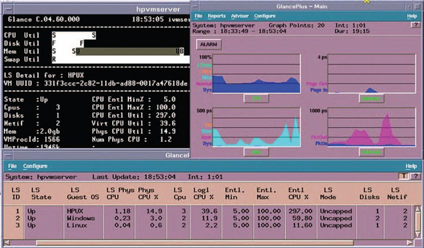
2.2.4 HP GlancePlus
HP GlancePlus provides system performance monitoring and diagnostic capabilities. It
enables examining system activities, identifying and resolving performance bottlenecks,
and tuning the system for more efficient operation. HP Performance Agent software
collects and maintains history data of the system’s performance and sends alarms of
performance problems. It allows the user to pinpoint trends in system activities, balance
workloads and plan for future system growth. HP GlancePlus Pak combines the real-
time diagnostic and monitoring capabilities of HP GlancePlus with the historical data
collection and analysis of HP Performance Agent software. The system uses rules-based
diagnostics. The system performance rules can be tailored to identify problems and
bottlenecks. Alarms can be based on any combination of performance metrics, and
commands or scripts can be executed for automated actions. GlancePlus displays real-
time system performance and alarms, summaries of real-time overview data, and
diagnostic details at system-level, application-level and process-level.
132. Background and state-of-the-art
Figure 3. Snapshot from the HP Glance Plus user interface. Source HP GlancePlus software
Datasheet.
2.2.5 Netuitive Service Analyzer
Netuitive Service Analyzer is an adaptive performance management tool that provides
automated real-time analysis. Netuitive Service Analyzer self-learns its operating
environment and correlates performance dependencies between system elements. It
identifies the relationships between components in business services across both
physical and virtual domains, silos and platforms. The system does not use manual
rules, scripts or dependency mapping. It uses statistical analysis techniques to identify
multiple, simultaneous anomalies and forecast conditions. Adaptive Behavior Profiles™
define every component’s range of normal behavior by time of day, day of week, or
season of the year. These profiles are used in creating alarms.
142. Background and state-of-the-art
Figure 4. Netuitive Service Analyzer architecture scheme. Source Netuitive Service Analyzer
Brochure.
2.2.6 OpenService InfoCenter (NerveCenter)
OpenService offers integrated security information management and network fault
correlation applications that link events from multiple sources to find the threat signal
using real-time root cause analysis. Their system consists of three modules of
OpenService InfoCenter™: LogCenter™, ThreatCenter™, and NerveCenter™ that are
unified with a common collection engine and user interface. LogCenter stores log and
event data from all its inputs for long-term reporting. ThreatCenter sifts incoming data
152. Background and state-of-the-art
looking for matches to its pre-defined risk models, identifying system-wide security
issues that might not reach the threshold of any single network or security device.
NerveCenter supplies a framework that enables customizing its functionality to match the
way the services are configured. ThreatCenter is based on out-of-the-box finite state
algorithms. NerveCenter has some out-of-the-box correlation capabilities that operate
without customer input regarding services and their component elements, but achieving
true service awareness requires that NerveCenter be informed about which elements
support each service. NerveCenter looks at all network layers, correlating problems with
a model that maps services to service elements. OpenService claims that any network,
application, or service issue that can be signaled or periodically tested, can be
incorporated into NerveCenter for intelligent correlation.
Figure 5. OpenService InfoCenter architecture scheme. Source NerveCenter Service Management
Concepts greenpaper.
2.2.7 Conclusions
Based on the brochure texts above it is not possible to rank these software tools. Nagios
and GroundWork Monitor are open source, others are commercial products. User
interfaces and monitoring architectures may look different but they probably contain
roughly the same functionalities. It is clear that the amount of data that these tools can
162. Background and state-of-the-art
produce easily grows rapidly. Hence, it is important to fine tune any such software in
order to not to produce huge amounts of useless data. The software developers cannot
do such a fine tuning beforehand, on the contrary, software developers attempt to make
everything possible. It is the task of the end user to decide what information is really
needed.
173. Observations from data – explorative approach
3. Observations from data – explorative approach
In this section we report some observations, with plots illustrating the phenomena, made
during the data exploration. The analyzed data has the following characteristics:
• The data is from several servers. Some of the servers are application servers
and the others are database servers.
• Data is available from 3 non-consecutive months (small changes in the
system have been made between the months and thus the results from
different months are not directly comparable).
• Time-series data contains originally almost 1000 attributes. However, only a
subset of attributes was chosen for the analysis.
• The data is stored in constant time intervals, usually 1 minute, but even, e.g.,
5 minute intervals.
• The data we used is not labelled, i.e., we did not have at our disposal ground
truth, data that would tell us which instances of data contain troublesome data.
• The variables used in the analysis included, e.g., indicators referring to
number of process, CPU load level, amount of memory and swap space, and
percentages of CPU time spent on user processes and system processes.
3.1 Differences in indicator types
There are clear differences in the measured indicators from several points of view. For
example, some indicators behave nicely and, as one might intuitively expect them to
behave, such as number of processes in Figure 6a. On the other hand, other indicators
are not so stable, but exhibit rather irregular behaviour such as Figure 6b. Furthermore,
some can have most of the time a constant value and only occasionally some other high
value such as Figure 6c. A relevant question related to this is how much information is
contained in a spike of the irregular indicator, or is the spike just noise emanating from
various non-severe reasons?
183. Observations from data – explorative approach
a) Number of processes.
b) CPU utilization (between 0% and 100%).
c) Number of pages swapped.
Figure 6. Differences in indicator types.
193. Observations from data – explorative approach
Another difference in the indicator types is the range of values. For those indicators that
measure something in percentages from a maximum, it is clear that the value will stay
(unless there is some measurement or calculation error) between 0 and 100. Also, for
indicators such as amount of free memory the value range is easy to state (between 0
and the amount of installed memory available for use). However, for other indicators
such as the number of processes the range of values is not so straightforward to state:
we have observed that the number of processes varies periodically around 400 but in the
measurement data it has sometimes gone up to about 1000 without any indication of a
problem.
One more aspect is the ability of an indicator to represent a harmful situation. As
stated before, the number of processes has been observed to go upto 1000 in our data –
and that has not actually been a harmful situation. However, if the number of processes
goes down close to 0, there is for sure something wrong. Thus, changes in the indicator
values in one direction might not be something to get worried about, whereas changes in
the other direction might clearly indicate a problem. The high number of processes as
such does not imply lack of resources in the same way as a high level of memory
consumption. Note also that the measurement agent itself is a process in the same server
system. This affects to such indicators as the number of processes or CPU load and
utilization. In some cases it is not possible to observe a value 0 in the data. However, it
is possible that the system has crashed and restarted between two consecutive polling
instants, especially if the period between has been 5 minutes.
3.2 Correlations between indicators
Several cases have been observed in the data in which there is clear correlation between
values of two indicators. An example is shown in Figure 7a visualizing the CPU
utilization (which measures how heavily the CPU is involved in processing currently)
and CPU load (which measures the number of processes in the kernel run queue). These
are clearly related (for understandable reasons): the higher the current CPU utilization
is, the more processes end up in the kernel queue. However, the number of processes in
the kernel queue depends also on other factors, e.g., how many processes were started
(offered load).
Another kind of correlation can be seen in Figure 7b, where the same indicator (idle
time percentage) is shown for two processor cores. The plot shows that, on the average,
when one core is idle, the other is as well – and the same applies when one core is
heavily loaded. This is due to the load balancing mechanisms, which are built in the
operating system itself. However, from the point of view of anomaly detection, removal
of redundant (correlated) indicators could be an issue. Also, the detection of anomalies
in the load balancing mechanism itself might sometimes be a useful use case.
203. Observations from data – explorative approach
a) Correlation between CPU utilization percentage and number of
processes in kernel run queue.
b) Correlation between percentages of time core A and B are idle.
Figure 7. Correlations in the data.
3.3 Seasonality
There are some natural periodicities that the indicators can be expected to exhibit in
server environment. For example, the hour of the day and the day of the week should
influence the indicator values and cause seasonality. Indeed, this can be clearly seen in
Figure 8, where the number of processes is shown for weekdays (Figure 8a and Figure
8c) and week-ends (Figure 8b and Figure 8d) separately. The area of variation for the
213. Observations from data – explorative approach
indicator values is heavily dependent on the hour of the day. The anomalies present in
the plots can be divided into two groups: ones that could have been detected with
constant thresholds (indicated with 1 in Figure 8) and the others, indicated by 2 in
Figure 8, that could not have been detected with constant thresholds. The latter would
have benefitted from time-dependent thresholds. However, some indicators do not have
similar seasonal behaviour such as the ones shown in Figure 8e–h.
600 1000
900
500
800
1
400 700
Processes (#)
Processes (#)
600
300
500
200 2 400
300
100
200
1
0 100
0 5 10 15 20 25 0 5 10 15 20 25
Hour of day (1..24) Hour of day (1..24)
a) Number of processes (weekdays). b) Number of processes (weekends).
6 6
x 10 x 10
7 16
2
6 14
1
5 12
Free memory
4 10
3 8
2 6
1 4
0 2
0 5 10 15 20 25 0 5 10 15 20 25
Hour of day (1..24)
c) Free memory (weekdays). d) Free memory (weekends).
223. Observations from data – explorative approach
100 100
90 90
80 80
70 70
CPU utilization (%)
CPU utilization (%)
60 60
50 50
40 40
30 30
20 20
10 10
0 0
0 5 10 15 20 25 0 5 10 15 20 25
Hour of day (1..24) Hour of day (1..24)
e) CPU utilization (weekdays). f) CPU utilization (weekends).
140 70
120 60
100 50
Pages swapped (#)
Pages swapped (#)
80 40
60 30
40 20
20 10
0 0
0 5 10 15 20 25 0 5 10 15 20 25
Hour of day (1..24) Hour of day (1..24)
g) Pages swapped (weekdays). h) Pages swapped (weekends).
Figure 8. Seasonality in indicators.
3.4 Anomaly or a consequence of one?
Anomaly detection in this study is based on indicator values. If the value of an indicator
deviates a lot from the average (or normal) value (by being too low or too high), it could
indicate an anomaly. However, consider the following example. In Figure 9, a time-
series of the number of processes is shown. There are some spikes both downwards and
upwards in the time-series. The biggest spike (upwards, indicated by 2 in the picture) is
easily – and erroneously – considered to be an anomaly. Actually, it is only a consequence
of one event a while before it (small spike downwards, indicated by 1). The small spike
downwards could actually have reached the zero level (i.e. number of processes could
233. Observations from data – explorative approach
have been zero for some time). However, due to the indicator averaging time step of 1
minute, the averaged indicator value does not go down to zero.
Figure 9. Anomaly and its consequence.
3.5 Localization of the problem
By monitoring several inter-connected servers, it is possible to gain insight into the root
cause of the anomaly. In Figure 10, an indicator time-series (number of processes) is
shown for two servers in the same network. By comparing the two time-series we
observe that some of the features are similar in both of them whereas others are present
only in one of them. Examples of the former case are the apparent seasonality (daily)
and drop in the indicator values before the date 12.5. (indicated by 2). An example of
the latter case is the rising trend within the seasonality (indicated by 1) present only in
server A time-series; i.e., the indicator value in server B returns always to the baseline
level of about 200 after each daily cycle but in server A the baseline level tends to be
higher for the subsequent day.
243. Observations from data – explorative approach
a) Number of processes in server A.
b) Number of processes in server B.
Figure 10. Comparison of servers.
3.6 Changes in the state of the system
Sometimes there can be clear changes in the system state that will prevail for a longer
time. Such changes are illustrated in Figure 11. First, Figure 11a shows total amount of
swap and free swap space as a function of time – a clear drop in both of them can be
observed at one instant of time (marked B in the other plots). The graph of CPU
utilization (Figure 11c) shows clear change in the lower indicator level at instants of
time A and B. Number of processes drops abruptly at the time instant B (shown in
Figure 11b). These changes are further illustrated with the number of processes and the
amount of free memory in Figure 11d). Two clusters are marked into the picture: all
observations before the time instant B fall into the second cluster. However, after B, the
system can be in either state 1 or state 2. The roughly linear relationship between the
number of processes and amount of free memory in, e.g., cluster 2 is understandable and
indicates the border of the feasible region in which the system can stay.
253. Observations from data – explorative approach
7
x 10
6
5
4
Swap (free or total)
3
2 Free swap
Total swap
1
0
02/11 09/11 16/11 23/11 30/11
Date
a) Total swap space and amount of free swap as a function of time.
900
800 A B
700
600
Processes (#)
500
400
300
200
100
0
02/11 09/11 16/11 23/11 30/11
Date
b) Number of processes. Two instants of time marked by red and dotted vertical lines.
263. Observations from data – explorative approach
100
90 A B
80
70
CPU utilization (%)
60
50
40
30
20
10
0
02/11 09/11 16/11 23/11 30/11
Date
c) CPU utilization. Two time instants marked by red and dotted vertical lines.
900
Before A
800 After A, before B
After B
700
600 2
1
Processes (#)
500
400
300
200
100
0
0 1 2 3 4 5 6
Free memory 7
x 10
d) Indicator values before time instant B (i.e. green and red) occur only in the cluster
2 in the plot (i.e. cluster 1 consists only of observations after instant of time B).
Figure 11. Changes in the system state.
274. Analysis methods and examples
4. Analysis methods and examples
4.1 Anomaly detection based on SOM analysis
In this test case we have shortly studied the accuracy of Self-Organizing Maps (SOM)
based anomaly detection in server log data anomaly detection. The aim is to show the
applicability of multivariate SOM based anomaly detection in monitoring and at the
same time to compare the SOM method with simple threshold monitoring of single
measurements.
We selected the measurements from January 2008 as our test cases because we previously
detected a clear problem situation in that data set in our initial data review. We used a Matlab
toolbox called SOM toolbox 2.0 (http://www.cis.hut.fi/projects/somtoolbox/download/) and
common Matlab visualization tools in our tests. In the selected data set there are 11
explanatory variables that have been measured on a minute interval. The date field has
been broken down to three components: day, hour and minute. We used the hour
component as a temporal explanatory variable in the tests. We performed the test for
data representing ordinary working hours (working days (Monday through Friday) and
normal working hours (7–17)) as it was previously found that there is a clear difference
in the behaviour of the log data outside of these times. Our test data consists of 660
samples on January 18th. Also, we selected the rest of the samples within the study
period as the training set containing 5719 samples.
The data set was inspected visually for the selection of the training data set. Part of
the variables have very rapidly fluctuating values, like variable Waiting_time (Figure 12);
part of the variables are more steady but contain occasional peaky periods, like variables
Number-of-user-processes (Figure 13), Number-of-other-processes (Figure 14), Free-
swap (Figure 15) and Free-memory (Figure 16). In these figures we also show alarm
thresholds (red lines) for these univariate cases. The thresholds have been set to the
mean value plus/minus 2.28 times the standard deviation. The value 2.28 has been
chosen because generally it seemed to produce a suitable amount of alarms.
An enhanced method would be to compute hourly alarm limits for the data based on
the logged values. Another improvement would be to set the alarm thresholds based on
284. Analysis methods and examples
the percentiles of the distribution, i.e., at the P02 and P98 percentiles representing the
values where 2% of the values are below P02 value and 2% above the P98 value.
Another enhancement would be to define each variable a unique std_multiplier value.
These enhancements have not been tested in this study.
Extreme values of component13 (Waiting-time), with stdmultiplier=2.280000e+000
70
60
50
40
30
20
10
0
-10
-20
0 0.5 1 1.5 2 2.5 3 3.5 4
4
x 10
Figure 12. Fluctuating value range in a measurement (variable waiting time).
294. Analysis methods and examples
Extreme values of component9 (Number-of-user-processes), with std
m
ultiplier=2.280000e+000
900
800
700
600
500
400
300
200
100
0
0 0.5 1 1.5 2 2.5 3 3.5 4
4
x 10
Figure 13. Variable Userprocesses and statistically selected anomaly thresholds.
Extreme values of component10 (Number-of-other-processes), with std
m
ultiplier=2.280000e+0
90
85
80
75
70
65
60
55
50
45
0 0.5 1 1.5 2 2.5 3 3.5 4
4
x 10
Figure 14. Variable Other processes and statistically selected anomaly thresholds.
304. Analysis methods and examples
Extreme7 values of component14 (Free-swap), with stdmultiplier=2.280000e+000
x 10
2.5
2
1.5
1
0.5
0
0 0.5 1 1.5 2 2.5 3 3.5 4
4
x 10
Figure 15. Variable Free swap and statistically selected anomaly thresholds.
Extreme 6values of component8 (Free-memory), with stdmultiplier=2.280000e+000
x 10
15
10
5
0
0 0.5 1 1.5 2 2.5 3 3.5 4
4
x 10
Figure 16. Variable Free memory and statistically selected anomaly thresholds.
314. Analysis methods and examples
After selecting the training and the test data sets we have created the anomaly detection
model by teaching a relatively small SOM map based on the training data. For the
modelling we have at first normalized the variables to have a 0 mean and standard
deviation of 1 in order to make all the variables equally influential with the Euclidean
distance metric. With some variables, that are far from a Gaussian form, additional
scaling would be beneficial but this has not been tested here. The used anomaly
threshold has been selected statistically based on the distribution of the training data
anomalies (in this test we have used the mean and the third multiple of the standard
deviation, µ + 3δ). The attached Figure 17 illustrate graphically the componentwise
distribution of the SOM neurons. We can see that some of the values of the explanatory
variables behave similarly over the neurons, e.g., CPU utilization and CPU load or
System time and System time percentage.
U-matrix Day Hour Minute
1.71 23.5 12.9 30.9
1.16 19.9 11.8 29.5
0.608 16.3 10.7 28.1
d d d
Cpu-utilization CPU-load System-time User-time
64.4 2.8 25.9 39.7
44.8 2.03 17.9 27.5
25.2 1.25 9.82 15.3
d d d d
Free-memoryNumber-of-user-processes
Number-of-other-processes
System-time-percentage
4.84e+006 398 77.8 27.9
4.09e+006 343 76.7 20.4
3.33e+006 288 75.6 13
d d d d
User-time-percentage Waiting-time Free-swap
38.2 9.52 1.51e+007
26.3 6.96 1.43e+007
14.4 4.41 1.35e+007
d d d
SOM 29-Dec-2008
Figure 17. Component level visualization of a learned SOM map.
The created model has been tested on the test data set in order to find clearly anomalous
samples as compared with the normality model. Figure 18 illustrates the anomaly scores
for the test data samples in the upper subplot and the values of some promising
explanatory variables in the lower subplot. Scores that have been considered anomalous
have been marked by a red sphere. In the lower subplot such values, that have been
statistically considered to be anomalous on a univariate case, has been circled. Visually
we can observe that some of the SOM anomalies can be explained by the univariate
324. Analysis methods and examples
values but none of the explanatory variables can by itself explain all the anomalies. In
principle the univariate alarm sensitivity could be enhanced by lowering the threshold
value but this was found to cause a lot of false alarms in some of the variables.
By comparing the univariate alarms and the SOM anomalies more carefully one may
observe that in the test case by taking the union of the alarms of the four explanatory
variables, four alarms will be created. Three of them co-occur in the SOM anomalies.
SOM could identify 11 anomalies. Therefore the four variables could predict 27.3% of
the SOM anomalies with a 25% false positive rate. When we consider all the 11
explanatory variables we can explain 63.6% of the SOM anomalies but the false
positive rate has been raised to 68.2%. It is therefore clear that univariate component-
wise analysis does not produce fully similar results with the multivariate SOM analysis.
However, only a careful log data expert analysis and labelling of the different test
situations would allow one to determine how well the SOM anomalies match with the
interests of the experts. Also, the larger amount of alarms caused by univariate analysis
may actually be justified, and provide valuable hints of trouble spots and anomalies.
qes for the test data set
samples at empty tr neurons qes for the test data set
8 samples with too high BMU-wise QE
samples with too high QE
7
6
5
4
3
2
1
0
0 100 200 300 400 500 600 700
Number-of-user-processes
Number-of-user-processes too extreme
Number-of-other-processes
Number-of-other-processes too extreme
700
Free-memory
Free-memory too extreme
600
Free-swap
Free-swap too extreme
500
400
300
200
100
0
0 100 200 300 400 500 600 700
Figure 18. Anomaly detection results with the test case.
334. Analysis methods and examples
We can produce explanations of the SOM anomalies with the help of our anomaly
detection tool. For example, visually it was not possible to find an explanation for the
first anomaly in the figure based on the four explanatory variables. However, with the
help of an explanatory log (see Attachment A) we have found that the most influencial
explanatory variables are CPU-load, User-time, User-time-percentage and CPU-
utilization. Thereby, it seems that the anomaly has been caused by an unusually high
user activity and the related high CPU load at that time. The combined deviation of
these four variables is summarized in the SOM anomaly score and therefore the
anomaly is being highlighted better than in the fundamentally 1-dimensional analysis.
Based on our tests the multivariate analysis of the explanatory variables using SOM
clustering detects more anomalies than the univariate tests could produce together.
However, we have not had a complete set of expert analyzed and labelled measurement
data at our disposal. This prevents us from saying, which of the anomalies are actually
problematic and require expert intervention. Anyhow, it seems that SOM anomaly
detection could benefit log data monitoring as a part of the early alarm system. The
univariate variables could also be monitored with the fixed alarm levels as well.
345. Example use cases
5. Example use cases
5.1 Identification of need for updates and verification of their
impact
One practical use case is how to identify and to decide, when to upgrade the capacity of
a system. This can mean, e.g., adding more memory or disk space to a server.
Adding the capacity too early when it is not yet needed would imply additional costs
without any benefit. Failing to add capacity on time might imply poor performance for
the system or even difficulty in detecting errors in the system. (Errors might manifest
themselves in other places that in the bottle-neck part of the system, making it even
more difficult to detect the root cause).
Another related use case is the verification of the impact of the system upgrade. If,
e.g., more memory or disk space has been added to the system, it would be good to be
able to provide a quantitative proof of the improvement in system performance.
5.2 Introduction of a new application
A relevant use case is the estimation of the impact of a new application on the load of a
server. It would be desirable to know, if the current system can cope with the load
caused by a new application before the application is introduced.
The application provider might give some guidelines on the requirement for the
system that runs the application. However, due to varying configurations, the guidelines
might be just indicative and more accurate assessment would be required.
One approach would be to evaluate the system performance with a subset of the
future users of the application to be introduced, and to attempt to estimate, based on
that, the impact of all the users (using the application) on the system performance.
355. Example use cases
5.3 Indication of the normal situation
A basic use case in anomaly detection is to be able to see the normal or reference
situation together with the current situation. The normal situation is typically time
dependent (e.g. hour of the day, day of the week), and thus that should be taken into
account when showing the normal situation to the end-user.
5.4 Trend detection
Temporal characteristics of the indicators are important not only from the point of view
of seasonal or periodic aspect, but also from the point of view of trends. Downward
trend in the amount of free memory gives a reason to upgrade the amount of system
memory. Of course, it should be verified first that the downward trend is indeed due to
constantly growing memory consumption, and not due to seasonal or periodic phenomena
nor some individual mal-performing process, that keeps allocating more and more
memory without releasing it.
The trend visualization or indication can be used as an aid to determine, when certain
actions need to be performed for the database.
366. Conclusions, ideas and challenges
6. Conclusions, ideas and challenges
In this preliminary study, we have reviewed the state-of-the-art related to server
monitoring and carried out some analyses based on real server log data. Furthermore,
during the study we discussed with experts of the field to identify real end-user needs.
Some issues that were observed to be relevant and would deserve further investigation
are e.g.:
• Labelling of data. In many anomaly detection studies, it is assumed that data
from normal situation is available for building the normality model. However,
usually the recorded data contains both measurements from normal situations
as well as from anomalous situations. Furthermore, labels attached to the
measurement data (indicator time-series) are not often available. Thus, the
algorithms and methods used for anomaly detection should be able to cope
with this kind of unlabeled data without making the assumption that the
training data representing only normal situations is available.
• Changes in the system. Upgrades to the system are sometimes made. Updating
frequency influences the normality model. Some changes had been made to the
system during the measurement periods and between them. The anomaly
detection algorithms should be able to take these changes into account.
• Architectural issues. The collection of indicator data from the server influences
itself the server performance and this should be taken into account in some
cases. Also, the fact that the data from the server is collected using an agent
running the monitoring target server implies, that no monitoring data can be
obtained, while the target server is being booted. With, e.g., 1 or 5 minute data
collection and averaging time step, booting manifests itself in the data in, e.g.,
close to zero (but often non-zero due to averaging) values for number of
processes indicator.
376. Conclusions, ideas and challenges
• Algorithms and experts. The expert is clearly needed in the anomaly detection
process. An instance can be detected as an anomaly by the system (algorithm)
when it is actually only a consequence of an anomaly – this kind of behaviour
was observed in this preliminary study from real data. The server log data does
not necessarily have enough information to be used for making the ultimate
decision about the severity of a detected anomaly – rather the other way
around, the anomaly detection system should be an auxiliary tool for the
expert. The expert would be the one saying the last word.
• Trends and seasonalities. Natural seasonalities (daily, weekly) are clearly
present in some indicators and the anomaly detection algorithms should utilize
these. Furthermore, superimposed trends can give relevant information about
changes in the system and by comparing data from several servers, insight into
the origin of the issue can be gained.
• Scaling and normalization. As observed in this preliminary analysis, there are
differences between the types of input variables. Some variables contain large
spikes, but they are often close to zero in value. The spikes influence the
calculation of the variance and thus the normalization, if the straightforward
approach of normalizing to zero mean, unit variance is adopted. Better approach
could be to apply some transformation (e.g. extract logarithm) or to leave out
the spikes from the variance calculation.
38References
References
1. Ziv, J. On Classification with Empirically Observed Statistics and Universal Data Compression,
IEEE Transactions on Information Theory, Vol. 34, No. 2, March 1988.
2. Trettel, E.L. Forecasting Database Disk Space Requirements: A Poor Man’s Approach,
Prepared for the CMG Conference Committee 32nd Annual International Conference
of The Computer Measurement Group, Inc., December 4–9th 2006, Reno, Nevada,
http://regions.cmg.org/regions/mspcmg/Presentations/Presentation03.doc.
3. Perng, C.-S., Ma, S., Lin, S. & Thoenen, D. Data-driven Monitoring Design of Service Level
and Resource Utilization. 9th IFIP/IEEE International Symposium on Integrated Network
Management, 2005. 15–19 May 2005. http://ieeexplore.ieee.org/iel5/9839/31017/
01440773.pdf?tp=&isnumber=&arnumber=1440773.
4. Knobbe, A., Van der Wallen, D. & Lewis, L. Experiments with data mining in enterprise
management. In: Proceedings of the Sixth IFIP/IEEE International Symposium on
Integrated Network Management, 1999. Distributed Management for the Networked
Millennium. http://ieeexplore.ieee.org/iel5/6244/16698/00770694.pdf?tp=&isnumber=&
arnumber=770694.
5. Yamanishi, K. & Maruyama, Y. Dynamic syslog mining for network failure monitoring.
International Conference on Knowledge Discovery and Data Mining. Proceedings of
the eleventh ACM SIGKDD international conference on Knowledge discovery in data
mining, Chicago, Illinois, USA. Industry/government track paper, 2005. Pp. 499–508.
ISBN 1-59593-135-X.
6. Renesse, R. Van, Birman, K.P. & Vogels, W. Astrolabe: A robust and scalable technology for
distributed system monitoring, management, and data mining. ACM Transactions on
Computer Systems (TOCS), Vol. 21, Issue 2 (May 2003), pp. 164–206. ISSN 0734-
2071.
39Appendix A: Explanations for some of the anomalies detected by the SOM method
Appendix A: Explanations for some of the
anomalies detected by the SOM method
Reasons for anomaly for the test data samples (11).
component_id component_name distance (test_value - neuron_value)
anomaly_id=1, data_id=192
5 CPU-load 3.718035 (4.894010 - 1.175974)
7 User-time 2.415240 (3.287868 - 0.872627)
12 User-time-percentage 2.300688 (3.193118 - 0.892431)
4 Cpu-utilization 1.921735 (3.220819 - 1.299084)
14 Free-swap -1.222020 (-1.384683 - -0.162663)
13 Waiting-time -1.184677 (-1.040180 - 0.144497)
8 Free-memory -0.817804 (-0.715234 - 0.102570)
9 Number-of-user-processes 0.787942 (0.888777 - 0.100835)
10 Number-of-other-processes 0.638121 (0.710480 - 0.072359)
11 System-time-percentage 0.347103 (1.698949 - 1.351846)
6 System-time 0.114685 (1.475803 - 1.361118)
anomaly_id=2, data_id=253
11 System-time-percentage 4.585687 (5.937533 - 1.351846)
8 Free-memory -2.475246 (-2.372677 - 0.102570)
6 System-time 2.453815 (3.814934 - 1.361118)
4 Cpu-utilization 1.380764 (2.679848 - 1.299084)
14 Free-swap -1.222020 (-1.384683 - -0.162663)
10 Number-of-other-processes 0.982804 (1.055163 - 0.072359)
13 Waiting-time -0.656987 (-0.512491 - 0.144497)
12 User-time-percentage -0.640461 (0.251970 - 0.892431)
9 Number-of-user-processes 0.360863 (0.461698 - 0.100835)
7 User-time 0.331135 (1.203763 - 0.872627)
5 CPU-load 0.150210 (1.326184 - 1.175974)
A1Series title, number and
report code of publication
VTT Research Notes 2480
VTT-TIED-2480
Author(s)
Sami Nousiainen, Jorma Kilpi, Paula Silvonen & Mikko Hiirsalmi
Title
Anomaly detection from server log data
A case study
Abstract
This study focuses on the analysis of server log data and the detection and potential
prediction of anomalies related to the monitored servers. The issue is relevant in many
mission-critical systems consisting of multiple servers. There it is favourable to be able
detect and even foresee problems to be able to react promptly and apply required
corrections to the system.
In this study, we have done off-line analyses based on pre-recorded data. In reality, if the
objective is to come up with solutions for detecting anomalies in real-time, additional
requirements and constraints would be imposed on the algorithms to be used. For example,
in on-line situation, higher requirements on the performance of the algorithm and on the
amount of historical data available for the algorithm would exist. However, we do not
address those issues in this preliminary study.
In addition to the analysis of real data, we have interviewed experts that are working on
the server-related issues on a daily basis. Based on those discussions, we have tried to
formulate practical cases, for which some algorithms and tools could provide practical utility.
ISBN
978-951-38-7289-2 (URL: http://www.vtt.fi/publications/index.jsp)
Series title and ISSN Project number
VTT Tiedotteita – Research Notes 13674
1455-0865 (URL: http://www.vtt.fi/publications/index.jsp)
Date Language Pages
April 2009 English 39 p. + app. 1 p.
Name of project
IPLU-II, Lokidata
Commissioned by
IPLU-II: Tekes, VTT, BaseN, CSC, Digita, Finnet, Fortum, HVK, LVM, NSN, TeliaSonera
Lokidata: VTT
Publisher
anomaly detection, data mining, machine learning, VTT Technical Research Centre of Finland
SOM, self-organizing map, IT monitoring, server log P.O. Box 1000, FI-02044 VTT, Finland
file, CPU, memory, process Phone internat. +358 20 722 4520
Fax +358 20 722 4374You can also read