Smartphone adoption, technology subsidies and complementary markets
←
→
Page content transcription
If your browser does not render page correctly, please read the page content below
Smartphone adoption, technology subsidies and complementary
                                                 markets

                                               Vatsala Shreeti∗
                                     Toulouse School of Economics
                                  DRAFT - PLEASE DO NOT CITE

                                                May 7, 2021

                                                   Abstract

          A vast majority of mobile phone users in developing countries continue to use low quality
      devices(feature phones) despite increasing affordability of smartphones, rising per capita income
      and declining cost of telecom services. Digitization of the economy is one of the main policy
      goals of many governments and the persistence of feature phones is especially problematic as
      more public services move online. By using a structural model of consumer demand of mobile
      handsets in a mixed logit framework, this paper tracks the adoption of smartphones in India
      between 2007 and 2018. Specifically, this paper evaluates two research questions i) What are
      the key barriers to smartphone adoption in India? ii) What types of policies can be used to spur
      adoption? I use the estimated structural parameters of utility to conduct two counterfactual
      simulations to answer these questions. I find that increasing competition in the services market
      (and thus reducing data expenditures) led to a 12.7 percentage point increase in smartphone
      adoption. As a preliminary answer to the second research question, I find that in order to have
      a 10 percentage point increase in smartphone adoption, a subsidy of $ 16 is required. Crucially,
      the gains from the same level of subsidy are higher in later periods.

  ∗
    I am thankful for the inputs and suggestions from Isis Durrmeyer, Daniel Ershov, Renato Gomes and Stephane
Straub. Frequent conversations with and inputs from Ana Gazmuri have also contributed meaningfully to this paper.
I thank the Indian Council for Research on International Economic Relations and LIRNEAsia for making the required
data available to me.

                                                       1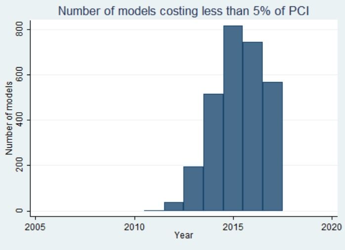
Introduction

Digital communication technologies have emerged as the new vehicle for development in the last
two decades in many of the emerging economies of the world. Governments as well as stakeholders
from the private sector have taken a keen interest in developing infrastructure for the transition
to a well-functioning digital economy. India has followed the same path and is now the second
largest market in the world for mobile telephony as well as internet services.1 While the mobile
phone revolution in India has been one of the biggest successes of the last decade, the migration
from low quality feature phones to smartphones has not taken off as widely as expected, despite
the increasing affordability (on average) and increasing variety of smartphones, and declining costs
of telecommunication services. The market for handsets continues to be dominated by feature
phones2 that accounted for more than 57% in 2018 by volume of sales3 , driven largely by the rural
and semi-urban populations.

  In this paper, I study the evolution of the handset market in India between 2007 and 2018. I use
a structural model of discrete choice to estimate consumer demand for handsets over this period.
To do this, I make use of novel proprietary handset level data published by the International
Data Corporation (IDC). I allow consumers’ choice of handsets to depend on their income through
heterogeneous price elasticities of demand. To do this, I combine the IDC data set with percentile
wise data on income distribution from the World Inequality Database (WID). Additionally, to
incorporate the effects of competition in the complementary market of mobile services and capture
usage of the device, I employ data on the cost of mobile internet from the Telecom Regulatory
Authority of India (TRAI). To obtain the structural parameters of consumer utility, I estimate
consumer demand under a random coefficients nested logit model using non-linear GMM. In ongoing
work, I use micro data from a new household survey provided by LIRNEAsia to incorporate income-
based heterogeneity on usage of devices.
   1
     https://en.wikipedia.org/wiki/ListofcountriesbynumberofInternetusers
   2
     Feature phones provide basic services like voice calling, SMS, and basic Internet browsing often at low speeds.
They typically do not have additional applications in the way that smartphones do.
   3
     Author’s calculation from aggregate sales data, recent household survey evidence from Financial Inclusion Insights
and LIRNEAsia puts this number even higher at 71%.

                                                          2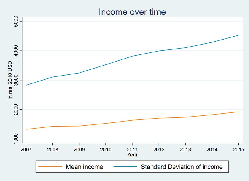
I use these parameters of utility to conduct counterfactual simulations to answer two main re-
search questions: i) What are the main barriers to smartphone adoption in India? ii) What type
of subsidy policies can be implemented in order to encourage adoption of smartphones? In order
to answer the first, I implement counterfactual policy simulations that allow me to decompose the
contribution of income, product variety, competition in the complementary data services market
and entry of Chinese products to the smartphone adoption trajectory (ongoing). To answer the
second research question, I conduct counterfactual policy simulations that evaluate subsidy pro-
grams. I consider the following types of subsidy programs - a flat subsidy for all smartphones, and
a targeted subsidy for smartphones for the bottom 30% of the income distribution, and a targeted
subsidy only for certain types of smartphones (ongoing).

  According to preliminary results, I find that competition in the services market had an important
role to play in increasing smartphone demand. In particular, increasing competition in the services
market in 2015Q1 (and thus reducing data expenditures) led to a 12.7 percentage point increase
in smartphone adoption. As a preliminary answer to the second research question, I find that in
order to have a 10 percentage point increase in smartphone adoption, a subsidy of $ 16 is required.
Crucially, the gains from the same level of subsidy are higher in later periods.

  Insufficient smartphone adoption is an important issue not just in India but most of the developing
world. Countries in East Africa and South Asia lag behind the developed world in smartphone
penetration, as well as behind the world average(GSMA, 2017).4 Smartphone adoption in the
developing world is all the more important because mobile devices provide the first access to the
internet for most people.5 Additionally, governments around the world are increasingly trying to
move public services online to facilitate more efficient utilisation of services by citizens. Efforts for
digitisation of the economy are only as good as the devices on which they can take place and thus,
persistence of low quality feature phones in the developing world requires further scrutiny.

  The case of India is particularly interesting as it lags behind in smartphone penetration compared
to countries like South Africa, Brazil, Mexico, Nigeria, which are at similar or lower stages of eco-
  4
    https://www.gsma.com/mobilefordevelopment/wp-content/uploads/2018/08/Accelerating-affordable-
smartphone-ownership-in-emerging-markets-2017w e.pdf
  5
    For example, in India, 97% of all internet access takes place through mobile devices.

                                                    3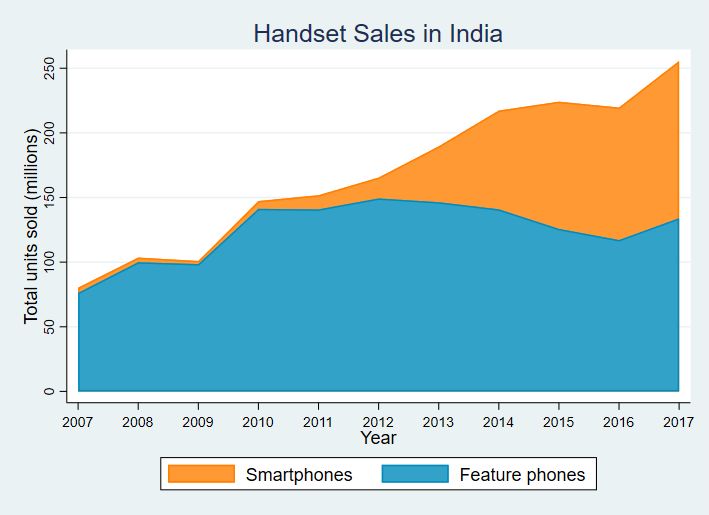
nomic development.6 The ongoing Covid-19 pandemic has brought the consequences of insufficient
smartphone adoption to light. Since the beginning of the pandemic last year, most of the schools
in India have been closed to physical presence and a large proportion of students (between 27%
to 56%) have no access to online schooling because they don’t own smartphones.7 More recently,
as the health infrastructure has crumbled during the second wave of the pandemic in India, many
citizens have primarily relied on social media and mobile applications to access resources online.
The majority of citizens that do not have access to smartphones or the internet are largely excluded
from these citizen-led relief efforts.8 These issues have made the question of insufficient smartphone
adoption all the more relevant and urgent for policy makers.

  The existing literature on the adoption of smartphones is limited. Most of the academic work
so far has concentrated on the economic and social impact of having access to telecommunications
services. Jensen (2007) evaluates the impact of efficiency gains in information sharing through
mobile phone connectivity in the fisheries sector in Kerala, India. Garbacz and Thompson (2007)
study the demand for telecommunication services in developing countries. Bjorkengren (2019)
studies network effects in the adoption of mobile phones in Rwanda until 2009, but does not evaluate
the handset market. Aker and Mbiti (2010) focus on the channels that link telecommunication
connectivity to economic development in Africa. In a similar analysis, Aker (2010) evaluates the
impact of mobile phone connectivity on price dispersion. A related strand of literature looks
at the impact of services like mobile money that can be used on feature phones. For example,
Jack and Suri (2016) evaluate the impact of mobile money on poverty in Kenya. Abiona and
Koppensteiner (2020) study the impact of mobile money adoption on consumption smoothing,
poverty and human capital investment in Tanzania. Bharadwaj, Jack and Suri (2019) evaluate the
impact of taking loans using mobile phones in Kenya. Most of this strand of literature concentrates
on the impact of using financial services that can be used on feature phones. As more sophisticated
mobile applications and platforms become are becoming relevant for the development process, it
may not be enough to concentrate only on the limited set of activities that can be undertaken
using feature phones. Ameen and Willis (2018) look at factors that shape gender differences in
   6
     https://venturebeat.com/2019/02/05/pew-south-korea-has-the-worlds-highest-smartphone-ownership-rate
   7
     https://indianexpress.com/article/education/about-56-pc-of-children-have-no-access-to-smartphones-for-e-
learning-study-6457247/;     https://www.hindustantimes.com/education/at-least-27-students-do-not-have-access-to-
smartphones-laptops-for-online-classes-ncert-survey/story-sp8nb0QZoBXXJ8ZsCLb3yJ.html
   8
     https://thewire.in/rights/india-covid-19-social-media-twitter-instagram-hospitals-beds-oxygen

                                                       4
smartphone usage in Iraq, but do not estimate demand for smartphones. The focus of governments
in developing countries has also been predominantly on mobile services and network infrastructure,
and less on the nature of devices being used in the digital economy. Papers that study the handset
market do so in the context of developed economies like the US (Fan and Yang, 2019; Wang, 2018;
Yang, 2019) and focus on questions of innovation and product proliferation.
In light of this, this paper makes three contributions. First, to the best of my knowledge,
this is the first paper to look at the transition from low quality feature phones to smartphones
using a novel panel data set over 12 years. Second, this paper contributes towards understanding
complementary markets by analyzing the impact of increased competitiveness in the mobile services
market on smartphones and having a demand model flexible enough to include heterogeneity in
usage. Finally, this paper contributes to the policy literature by evaluating (ex-ante) different
subsidy schemes to encourage smartphone adoption. The findings of the paper can thus inform
policy in developing countries to spur the digital economy.
The paper is organised as following: Section 1 maps the background of the industry between
2007 to 2018. Section 2 outlines the structural model of demand and provides a supply model of a
multi product oligopoly. Section 3 discusses the data and sample selection. Section 4 discusses the
estimation method. Section 5 provides the results of the estimation. Section 6 provides preliminary
results from ongoing counterfactual policy evaluations. Section 7 gives details of ongoing work and
section 8 concludes.
1 Background of the Industry
1.1 Market level descriptive evidence
As of 2017, there are 47 brands and 951 models of mobile phones available in the market suggesting
a large choice set for consumers. The market can be segmented into two groups - smartphones and
feature phones. Feature phones are basic handsets that run on the ’RTOS’ operating system, and
can be used for voice calls, sending text messages, and a limited capacity for internet browsing.
Smartphones, on the other hand, have sophisticated operating systems, partial or full touchscreens,
5and a wide varity of internet enable applications.9 Over the 12 year period between 2007 and 2018,
the pecking order of companies has been continuously changing.10 There has been considerable
entry and exit over most of the period, although entry, exit and churn rates11 have declined over
time, pointing to a more stable market towards the end of the period of analysis12 . There have been
two noteworthy events that have affected the trajectory of the market- the entry of new Chinese
firms in the mid-price segment of smartphones starting in 2014, and the entry of a new 4G provider
in the data services market in 2016.
Table 1: Total number of companies and models by year
Year Companies Models
2007 27 405
2008 30 597
2009 37 691
2010 37 1007
2011 40 997
2012 43 1527
2013 42 1544
2014 50 2257
2015 50 2234
2016 50 1825
2017 47 951
2018 40 497
Total 14532
Sales13 The main data source for this section is market level data on sales, prices and characteris-
tics of handsets between 2007Q1 to 2018Q2 published by the International Data Coporation (IDC).
At the beginning of the period in 2007 and until 2010, between two and three firms accounted for
approximately 70% of the total sales, with Nokia emerging as the market leader. Subsequently,
the market became less concentrated in terms of total sales, with 6–8 companies accounting for the
same 70% of total sales.14 The sales data also show a significant increase in the market shares of
Indian companies, particularly between 2012 and 2015.15 ,16 Most of these Indian companies entered
9
RTOS stands for real time operating system
10
Table 4 and 5 in the appendix provide details of company rankings by sales and value
11
Churn rate is the sum of entry and exit rates and is a crude indicator of the dynamics of the industry
12
Details in Figure 3 in the appendix
13
Since the data does not cover the entire year of 2018, the descriptive statistics are provided only until 2017 in
this section and the next.
14
Tables 9 and 10 in the appendix provide the ranking by sales of the top 8 companies.
15
The Indian companies are marked in red and the Chinese companies are marked in blue in tables 4, 5 6 in the
appendix.
16
Micromax, Intex, Lava, Spice, Karbonn- marked in red in tables 4 and 5 in the appendix.
6the market in 2009 and by 2015 accounted for over 30% of the total sales of the market. Prior
to entering the market as independent firms, all of them were distribution partners of established
global firms, and offered a cheaper alternative to the existing smartphones as well as to existing
feature phones. Between 2007 and 2017, the share of feature phones relative to total sales of all
handsets has been declining, even though it still accounts for over 50% of the market. Interestingly,
following the entry in the telecom services market, the share of feature phones increased in the last
year of the period. This increase was largely driven by the entry of a new type of product (hybrid
4G feature phones) in 2017.In addition to the basic functionalities (voice calling, SMS, limited
internet browsing), these hybrid 4G feature phones were bundled with the services of Reliance Jio
and come with a few pre-installed mobile applications (notably Whatsapp, Facebook) and offer a
walled-garden experience to accessing the internet. In terms of hardware, they are still keyboard
based with small screen sizes and do not have touch screen capabilities.
Figure 1: Volume of sales of handsets
Chinese Entry Since their entry in 2014, Chinese companies (Oppo, Vivo, Xiaomi, Oneplus)
have steadily gained market share, accounting for nearly 49% of the handset market by the end of
7period. As opposed to established Chinese companies (Huawei and Lenovo) that were present in
the market before 2014, the firms entering in 2014 targeted the mid-price segment of smartphones,
vastly expanding the choice set of smartphones. Through aggressive marketing, careful product
selection and exclusive contracts with retailers, these companies have managed to account for 75%
of the smartphone market today.17 18
Table 2: Sales by category in %
Product 2007 2009 2011 2013 2015 2017 2018
Feature phone 95.02 97.99 94.16 82.94 59.18 52.50 57.20
Smartphone 4.98 2.95 3.44 7.44 40.82 47.50 42.80
Prices Prices vary considerably over the 12 year period over time and across models. In the
paper, I normalize all the prices to 2010 real US dollars. The average real selling price (ASP) of a
handset has decreased from USD 291 in 2007 to USD 107 in 2018 (figure 2; table 11 in appendix).
The ASP of smartphones decreased from USD 618 in 2007 to USD 125.23 in 2018. Feature phones
also got cheaper over this time period with the ASP decreasing from USD 150 in 2007 to USD 11 in
2018. The ASP of smartphones as a proportion of the annual per capita real income has declined
from nearly 40% in 2007 to 8% in 2017. The median price of smartphones follows the trend of
mean prices quite closely, indicating increasing affordability. Moreover, the number of smartphone
models that cost less than 5% of the annual per capita real income has increased in number, with
as many as 567 in 2017. While these facts suggest that smartphones have become more affordable
in general, the trend in affordability might differ across different income levels of consumers as
income inequality has increased significantly over this period. Additionally, in figure 2, we notice
that towards the end of the period, the prices of smartphones start to increase again.
17
https://www.reuters.com/article/india-smartphones-idUSKBN29W1X3, last accessed on 3.05.2021
18
https://www.bbc.com/news/world-asia-india-50135050, last accessed on 3.05.2021
8Figure 2: Price of Handsets (2010 real USD)
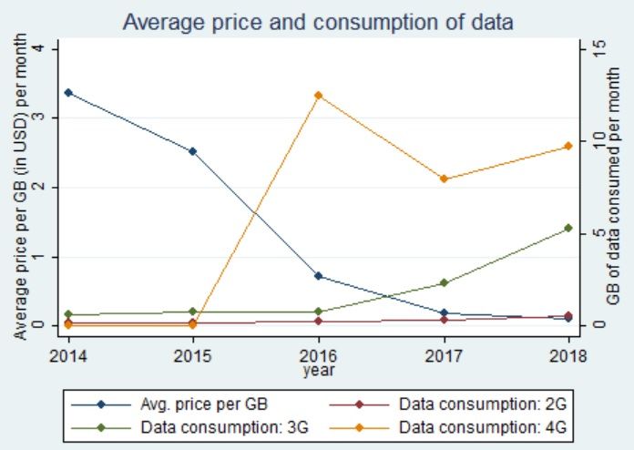
Entry in telecom services market In September 2016, with the entry of a new 4G service
provider (Reliance Jio) in the mobile internet services market, the landscape of the telecom sector
in India changed dramatically. Reliance Jio was the first operator to provide 4G mobile broadband
and internet based voice services. With near-zero pricing of its services, this led to the exit of
all but three incumbents (two of which subsequently merged)and a sharp increase in average data
consumption per subscriber and over 215 million new mobile broadband subscribers.19 The prices
of 2G and 3G mobile internet also dropped significantly in response to this entry. To put the
magnitude of the impact of this entry on internet prices in perspective, the average price of 1GB of
data dropped from USD 11 in 2015 to USD 5 in 2016 and USD 0.51 in 2018. Furthermore, India
jumped 154 places to be ranked the country with the maximum data consumption shortly after
September 2016.20 The fall in the prices of mobile internet was followed by product innovations in
the handset market (hybrid 4G feature phones) and introduction of device-operator bundling by
the entrant. These changes in the mobile services market are potentially important for smartphone
19
https://economictimes.indiatimes.com/industry/telecom/telecom-news/the-jio-effect/articleshow/65694564.cms
20
https://economictimes.indiatimes.com/industry/telecom/telecom-news/the-jio-effect/articleshow/65694564.cms
9adoption as they directly altered the cost of using mobile devices.
Figure 3: Average price and consumption of mobile internet
Income The income of individuals has been increasing over the time period of consideration but
so has the inequality. Based on data from the world inequality database, the mean annual real
income of an individual was $ 1338 in 2007 and increased to $ 2256 in 2018. The standard deviation
of the income distribution was $ 2840 in 2007 and this too increased to $ 5457 in 2018, pointing to
increasing inequality.
10Figure 4: Income and Income Inequality
1.2 Survey evidence on ownership and usage
While the previous section relied on aggregate data on prices and sales, in this section I provide
evidence on smartphone uptake and usage based on micro data at the individual level. I use the
nationally representative LirneAsia After Access Survey conducted in 2017. Around 61% of the
population has a mobile phone, of these 29.5% have smartphones, and 97% have pre-paid connec-
tions. The estimates of mobile phone and smartphone penetration are lower than in the aggregate
data because the latter over-estimates adoption – aggregate sales data don’t account for the same
individual buying multiple devices or individuals that replace their devices very frequently. Ev-
idence from the survey point to a substantial degree of heterogeneity in smartphone ownership
and smartphone usage. In table 3, I provide correlations between the probability of owning a
smartphone and individual demographics. I find that disposable income, years of schooling, us-
age expenditure, having a debit/credit card, having multiple SIM cards, having a computer, and
network effects are positively correlated with the probability of owning a smartphone.21 Usage of
21
Network effects are measured by the number of people in the respondent’s friend circle that have a smartphone
(maximum 5).
11the device (measured by monthly data expenditure) is positively correlated with income, years of
schooling, having a smartphone, and residing in an urban area.22 Only 18% of the people, and
25% of mobile phone users have used the internet. 60% of internet users use it at least once a day.
Of the people that use the internet, the most common uses are for social media (27.1%), email
(19.5%), entertainment (15.7%), education (15.41 %), and work (9.4%).
For the purpose of this paper, I concentrate on heterogeneity among consumers based on income.
India is an emerging economy with an expanding middle class, and both income and income in-
equality have increased over the time period of consideration. Income-driven heterogeneity is thus
likely to play an important role in understanding the adoption of smartphones and how people use
them, as suggested by figures 5 and 6.
Figure 5: Smartphone ownership across income classes in 2017
22
Table in appendix.
12Figure 6: Data expenditure across income classes in 2017
13Table 3: Probability of owning a smartphone
Smartphone
Women 0.0364
(0.227)
Age -0.0600***
(0.00970)
Married -0.363
(0.224)
Years of Schooling 0.102***
(0.0212)
Disposable Income 0.000101***
(0.0000386)
Hours worked 0.00307
(0.00364)
Bank account access -0.0412
(0.258)
Employed in agriculture -0.824***
(0.224)
Data expenditure 0.609***
(0.112)
Total telecom expenditure -0.00372
(0.0527)
Debit or Credit Card 0.295**
(0.109)
Number of SIMs 0.704***
(0.165)
Computer Ownership 0.983***
(0.277)
Network Effect 0.289***
(0.0664)
N 1975
pseudo R2 0.355
Standard errors in parentheses
* p < 0.05, ** p < 0.01, *** p < 0.001
142 Model
2.1 Demand Model
The adoption of a new technology like smartphones is affected by many factors (prices, income,
usage costs, time varying unobserved heterogeneity) and a structural model of consumer utility
is require in order to disentangle the effects of each of them. In this spirit, I adapt the random
coefficients nested logit (RCNL) model proposed by Grigolon and Verboven (2014). The RCNL
model of demand is useful when market segmentation is important in capturing unobserved hetero-
geneity. This should be the case in the handset market where consumers first decide the segment
of their purchase (feature phone or smartphone) and then decide which model to buy within these
segments.23
I consider T markets defined as each quarter of the period 2007Q1-2007Q2. The potential market
size of each market t is denoted by Mt . Each consumer i chooses a handset j in segment g sold by
company c in quarter t and gets the following indirect utility uijt from this purchase:
uijt = βxjt − αit pjt + γDigt + λc + λt + ξjt + ¯ijt (1)
Here,
σ
αit = (2)
Yit
and
¯ijt = ζigt + (1 − ρ)ijt (3)
Consumer i’s utility of purchasing handset j depends on a vector of product characteristics:
xjt , its price p in quarter t, the segment specific usage cost (captured by the data expenditure) D
incurred by the consumer in quarter t, company fixed effects λc that capture the average utility of
buying from a particular company, quarter fixed effects λt , and a measure of unobserved product
quality ξijt . The unobserved product quality might include characteristics like the color of the
phone, the shape of the phone etc which are not observed by the econometrician but are observed by
the consumer and the producer. A product j is defined as a unique bundle of handset characteristics.
23
Market segmentation can be captured using the standard mixed-logit demand model, however it is computation-
ally more costly compared to the RCNL model (Grigolon and Verboven, 2014)
15The model allows for individual level heterogeneity in the response to price changes through the
term αi specified by equation 2, Yi denotes the income of individual i. The non-linear parameter
sigma measures the marginal utility of income.
The error term ¯ijt takes into account market segmentation (g) and allows products within each
segment to be correlated with each other. This correlation is captured by the parameter ρ. ijt is
assumed to follow an extreme value type I distribution and ζigt has the unique distribution such
that ¯ijt is also extreme value type I. In this application, there are two market segments - feature
phones and smartphones, so g can take two values. Finally, an outside option is specified so that
the consumer can choose not to make a purchase in period t. The utility of the outside option is
normalized to zero:
ui0t = ξ0t + i0t = 0
The utility can be rewritten as a sum of three terms – the mean valuation δjt , the individual
specific heterogeneity µijt and an idiosyncratic consumer valuation (1 − ρ)ijt :
uijt = δjt + µijt + (1 − ρ)ijt (4)
where
δjt = βxjt + λc + λt + ξjt (5)
and
σ
µijt = pjt + γDigt + ζigt (6)
Yit
Using the extreme value distribution assumption, the probability that consumer i purchases a
product j in segment g in time period t is given as:
δjt +µijt
exp( 1−ρ ) exp(Iig )
πjt = Iigt
×
exp( 1−ρ ) exp(Ii )
where
Jg
X δmt + µimt
Iig = (1 − p) ln exp
1−ρ
m=1
16and
G
X
Ii = ln 1 + exp(Iigt )
g=1
Note that Jg is the number of products in segment g so that we have
G
X
Jg = J
g=1
Integrating the choice probabilities πijt over the distribution of observed demographics (Y ), we
obtain the aggregate market share of product j in period t:
Z
sjt (xt , pt , ξt ; θ) = πjt PY∗ (Y ) (7)
Yt
Here θ refers to the vector of non-linear parameters (σ and ρ) of the utility function.
2.2 Supply
The profits of firm f producing products Jf in period t with a marginal cost c are given by:
X
arg max (pj − cj ).sj (p)
pj :j∈Jf j∈J
f
The first order condition of this maximization problem in matrix form is:
(p − c) = ∆(p)−1 s(p)
Here, ∆ is the Jt × Jt matrix of intra-firm demand derivatives. Once demand has been estimated,
this first order condition can be used to recover estimates of marginal cost as follows:
c = p∗ − ∆(p∗ )−1 s(p∗ ) (8)
3 Data
Handset data The main data set that I use is published by the International Data Corporation
(IDC) and provides quarterly prices, sales and characteristics of mobile handsets sold in India over
17a 12 year period between 2007 until the second quarter of 2018. Data collection is bottom up- sales
and price data are collected from major vendors across the country. The data is provided at the
handset level, where a model refers to a unique bundle of handset characteristics and company.
There are a total of 9,534 models, 89 companies, and 27,730 observations (model-quarter) over the
twelve year period. The data set provides information on the following characteristics of handsets-
operating system, operating system variant, embedded memory, screen size, screen resolution, air
interface, communication technology (2G, 2.5G, 3G or 4G), processor speed band, processor core,
processor vendor, camera megapixels, RAM band, input method, GPS capacity, dual sim, form
factor, bluetooth capacity, waterproofing, primary memory card, dual rear camera, fingerprint
reader, display type, and NFC capacity.24
Sample Selection In the original data set, there are a group of very small companies (produc-
ing feature phones) clubbed together in a category called ”Others”. Since there is no additional
information available about the companies that are a part of this category, these observations are
dropped from the analysis.
Real prices The prices of handsets in the dataset are deflated by using the consumer price index
(CPI). The data for CPI is obtained from the IMF database.25 This is done in order to capture the
real purchasing power of consumers and to ensure that the analysis is not affected by time trends
in prices. The base year for the deflation is 2010. The prices are reported in US dollars as well as
the Indian rupee, and for most of the analysis the prices in US dollars are used.
1
Market size and Outside Option The potential market (Mt ) is defined as 8 of the total adult
working population of that year. Intuitively, this translates into the assumption that consumers
change their handsets every two years. The data for the annual population and the proportion of
the working population is obtained from World Bank Open Data.26
Expenditure on usage of device I proxy the usage of the device by the annual expenditure
on mobile internet. The monthly expenditure is the product of the amount of data consumed in
24
Input method refers to whether the phone is touchscreen or requires alphanumeric/QWERTY input through a
physical keyboard, or a combination of the two.
25
https://www.imf.org/en/Data
26
https://data.worldbank.org/
18gigabytes (GB) and the price paid per GB of data. I obtain the average cost of 1GB data for a user
from the Telecom Regulatory Authory of India’s (TRAI) report on wireless data services.27 . Since
this data is published annually, for the purpose of my analysis, I assume the price of 1 GB data to be
the same across all quarters of the year.28 TRAI also records information on the average gigabytes
of mobile data consumed per month classified by technology generation (2G, 3G and 4G).29 As
with the price of mobile data, I assume that data consumption does not change across quarters in
the same year. The data expenditure, thus, varies across years and across the technology type of
device (2G, 3G and 4G).
Table 4: Average monthly expenditure on mobile data in USD
Device type 2014 2015 2016 2017 2018
2G 0.47 0.50 0.17 0.05 0.05
3G 2.10 1.90 0.57 0.41 0.53
4G 0 0 8.94 1.43 0.97
This data is only available starting in 2014. In fact, the market for mobile internet gained mo-
mentum only after the 3G spectrum auctions in India which were held in 2010. This is further
corroborated by figure 4 which shows that the amount of data consumed per subscriber was neg-
ligible before 2011. This is taken into account in the demand model by including an interaction
term between the data expenditure and an indicator variable for the years after 2014.
Survey data on mobile internet expenditure To allow for heterogeneity in data expenditure,
I use the After Access Survey provided by LIRNEAsia.30 . This is a nationally representative cross-
section of 5069 households and individuals, conducted in 2017. One of the primary goals of the
survey is to record the device ownership and device usage behaviour. I use information on individual
income and monthly expenditure on data in order to model heterogeneity in usage of devices.
27
https://trai.gov.in/notifications/press-release/trai-releases-report-wireless-data-service-india, last accessed on
16.10.2020 at 2.30 p.m.
28
While proxy-measures for the cost of 1GB data (like Average revenue per user of operators from data services)
at the quarterly level are published by TRAI, these are often not entirely reflective of the cost of data that the user
faces.
29
https://main.trai.gov.in/sites/default/files/WirelessD ataS erviceR eport2 10820190 .pdf
30
LIRNEasia. 2019. AfterAccess Asia (data set). Colombo: LIRNEasia. The findings and opinions in this paper
are the author’s and not of LIRNEAsia
19Data on income One of the key objectives of the demand model in this paper is to capture the
heterogeneous response to prices based on consumer’s incomes. To do this, I construct the income
distribution of the population at the national level using data from the World Inequality Database
(WID).31 The WID provides the average income of each percentile of the population for the years
2007 to 2015 in nominal dollars. For consistency with the handset and data prices, I convert the
mean incomes to real USD 2010. I use this information in the simulated draws of consumers - I
simulate 100 consumers and assign to each the mean income of each of the 100 percentiles from
the empirical distribution. Each consumer is therefore assigned the mean income of this percentile.
Since the WID data is only available until 2015, I calculate the average income of all 100 percentiles
for the years 2016, 2017 and 2018 by assuming that incomes grow at the average rate of growth of
the period 2007-15. In effect, this means that the rate of growth of mean income between 2016-18
is assumed to stay constant. Allowing income heterogeneity to vary over years, albeit with the
constant growth assumption for the years 2016-18, is especially important for the Indian context
since mean income and income inequality have both been increasing over the years.
4 Estimation
I follow Nevo (2000) and Grigolon and Verboven (2014) to estimate model given in section 2.1.
Since producers take into account the unobserved product quality (ξjt in the demand model) when
they set prices, prices are endogenous to the demand system. To correct for the bias arising from
this endogeneity, I use instruments for price. Following the literature, these instruments functions
of the characteristics of competitor’s products and I denote them by h(z). Specifically, I use own-
product characteristics and the sum of other products’ characteristics within each segment. These
are relevant instruments for price as they affect the mark up of differentiated instruments. Only
one out of any set of instruments that have a correlation greater than 0.9 are selected to avoid
issues arising from multicollinearity. The main identifying assumption with a vector of instruments
Zjt is:
Cov(ξjt , Zjt ) = 0
I construct demand moments based on these instruments h(z) and estimate the demand model
31
https://wid.world/, last accessed on 16.10.2020 at 4 p.m.
20using non-linear GMM. A two stepped algorithm, as in BLP(1995), is used to retrieve the linear
parameters of utility in the first step and then conduct a search for the non-linear parameters(θ =
(σ, ρ)) so as to minimize the objective function:
min ξj θ0 h(zj )Ωh(zj )ξj (θ) (9)
θ
These parameters are then used to compute ∆, the matrix of intra-firm demand derivatives,
which is in turn used to retrieve the marginal costs from equation 8.
Estimation Algorithm The estimation algorithm follows BLP (1995) with one modification.
In the first step, for a given set of initial values of the non linear parameters, a unique δjt is found
through a contraction mapping by setting the observed market shares exactly equal to the market
shares predicted by the model. I use the modified contraction mapping proposed by Grigolon and
Verboven(2014) for the special case of RCNL. The δjt is used to construct ξjt from equation (3),
which is then used to construct the demand moments as in equation (6). In the final step, the GMM
objective function is minimized to estimate the parameters. Details of the estimation algorithm
and its implementation can be found in Nevo (2002).
Empirical Specification To construct the demand moments, the three terms of equation (4)
need to be specified. As per equation (5), the first term δjt contains a vector of device characteristics
xjt , brand fixed effects λc and quarter fixed effects λt . The device characteristics include the screen
size, operating system type, camera type, dual sim capacity, technology generation (2G, 3G, 4G),
screen type (touchscreen or bar), and memory. I also include an interaction between the technology
generation of the device and a linear time trend to control for changes in network coverage over time.
The second part of equation (4) introduces heterogeneity among consumers based on their in-
come, specifically allowing consumers with different incomes to have different responsiveness to the
price of a handset; and different usage (data expenditure) based on their income. In equation (6),
Yit refers to the income of individual i in year t, which is drawn from the empirical income distribu-
tion constructed using data from the World Inequality Database. Digt is the empirical distribution
of usage that assigns a level of data expenditure to each individual based on their income. Finally,
21the third part if equation(4), the idiosyncratic error term (1−ρ)ijt is assumed to follow an extreme
value type I distribution.
Note that in the current draft, I do not provide results and counterfactual policy
simulations for the case that includes income based heterogeneity in data expenditures
since it is work in progress. Instead, the results presented allow data expenditure to
vary across quarters and market segment.
Identification of parameters Following Nevo (2002), the mean utility parameters β̄ abd γ are
estimated by a linear projection, which is substituted in the GMM objective function. β̄ can be
recovered from the correlation between the market shares of the products and their characteristics
over time. The income distribution of consumers in the market changes substantially over 2007-
2018 as do the prices of products and this is the variation used to pin down the random coefficient
σ on the price variable. The variation in the combined market share of each segment over time is
used to identify the parameter ρ.
5 Results
The main results of the demand estimation are provided in table 5. The key parameter estimates of
interest are (σ), the nest coefficient (ρ) and the mean data expenditure coefficients for smartphones
and feature phones. A table containing the full results of the demand estimation can be found in
the appendix.
Price sensitivity The coefficient on Pjt /Yit (σ) is negative and precisely estimated. A value of
σ = −3.45 implies a mean price sensitivity (ᾱ) of -0.06 at the beginning of the period in 2007Q1 and
-0.04 at the end of the period in 2018Q1. Compared to a model of nested logit demand (ᾱ= -0.004)
which does not incorporate income heterogeneity of consumers, the absolute value of the sensitivity
to price is higher. This is consistent with the literature; models that do not incorporate consumer
heterogeneity underestimate the price sensitivity of demand. Additionally, the model specification
and parameter estimate of σ implies that individuals with higher income are less price elastic than
individuals with lower incomes. The price sensitivity of the poorest percentile of income is -0.28,
22which is several orders of magnitude than the price sensitivity of the richest percentile of income
at -0.009. A value of the nesting parameter this high suggests a high degree of substitution within
nests(feature phone and smartphone) as opposed to across nests. In other words, consumer tastes
for products within each nest are highly correlated with each other.
Table 5: RCNL demand estimation
Price/Income (σ) -35.4***
(4.16)
Nest 0.85***
(0.02)
Data Expenditure × SP 0.01***
(0.002)
Data Expenditure × FP -0.57***
(0.03)
Company FE yes
Time FE yes
Time trend × techology yes
Other charac. yes
N 27,730
Expenditure and income in real 2010 USD
Nesting parameter A value of ρ close to 1 implies strong within group correlations in substi-
tution patterns, and a value of ρ = 0 implies that segmentation of the market into groups is not
required. From table 3, the nesting parameter is estimated precisely at ρ = 0.85. This means that
segmentation of the market is important - in other words, smartphones are much closer substitutes
of other smartphones than they are of feature phones, and vice-versa.
Data expenditure parameters I use data expenditure as proxy for measuring usage of devices.
From table 3, we see that the data expenditure parameters are significant and precisely estimated.
As data expenditure is the product of data consumption (positively related to utility) and data
prices (negatively related to utility), the sign of the parameter is ex-ante ambiguous. For smart-
phones, increasing data expenditure increases utility, presumably because the utility gains from
higher data consumption outweigh the dis-utility arising from data prices. On the other hand, for
feature phones, which have low data consumption, increasing data expenditure decreases utility, as
the dis-utility of data prices outweighs the any utility gains from data consumption. As mentioned
previously, currently data expenditure varies only by the technology type of device and over quar-
23ters. Ongoing work attempts to introduce heterogeneity in usage which can just as important as
including heterogeneity in price sensitivities.
6 Counterfactual Policy Simulations32
I implement two sets of counterfactual exercises - the first set corresponds to the first research
question and attempts to determine the key determinants of smartphone adoption in India. The
second set of counterfactual policy simulations are normative and correspond to the second re-
search question. These simulations aim to provide policy strategies that can be used to encourage
smartphone adoption. In both of the cases, I provide results for simulations conducted in the first
quarter of 2015.
6.1 Demand Decomposition
In this section, I use the estimated structural parameters of utility in order decompose the deter-
minants of smartphone demand in India. This is done with the aim of identifying the key barriers
to smartphone adoption in India. More specifically, I quantify the effect of the following factors
on the adoption trajectory of smartphones : income, competition in the complementary telecom
services market, product variety in the handset market (ongoing) and the entry of Chinese phones
(ongoing).
6.1.1 Income and Smartphone Adoption
Income and affordability of smartphones are arguably the most important determinants of the
adoption trajectory. To disentangle the effect of income on smartphone adoption, I re-simulate the
market equilibrium in 2015Q1 by setting the counterfactual income distribution to be that of the
beginning of the period (2007Q1). The mean real annual income was $ 1338 in 2007 and $1941
in 2016. More precisely, this means recomputing the market equilibrium with the same choice
set and data expenditure but with lower income (31% lower on average) and lower inequality
of individuals. This implies that individual market shares are integrated over the counterfactual
income distribution.
32
This section is work in progress and results as well as the set up of the counterfactual simulations are continuously
updated
24Table 6: Income of 2007Q1 in 2015Q1
Original Counterfactual % change
Sum of inside shares 0.4461 0.4438 -0.5%
Sum of SP shares 0.1888 0.1871 -0.9%
Sum of FP shares 0.2573 0.2567 -0.2%
Mean price SP 140.58 147.62 4.9%
Mean price FP 17.9 18.34 2.4%
Proportion of SP 42.3% 42.1% -0.2%
I find that the reduction in income in 2015 to 2007 levels does not change market outcomes too
much. The total size of the market decreases by 0.5%, the smartphone market decreases by 0.9%.
Average price of smartphones increase by 4.9%.
6.1.2 Competition in complementary market
As mentioned previously, Reliance Jio entered the mobile internet market in 2016, and offered near
zero tariffs for using mobile data on handsets. The average price per GB of data came down from
USD 3.5 in 2015 to approximately USD 0.10 as of June 2018. In this counterfactual exercise, I try to
capture the extent to which competition in the data services market affects smartphone adoption.
I do this by allowing data expenditure in 2015Q1 to be equal to the post entry levels (thus, lower
than observed). Effectively, this means simulating a scenario where the services market was more
competitive in 2015 than actually observed.
Table 7: Data Expenditure of 2017Q1 in 2015Q1
Original Counterfactual % change
Sum of inside shares 0.4461 0.5783 29.6%
Sum of SP shares 0.1888 0.3184 68.6%
Sum of FP shares 0.2573 0.2599 1%
Mean price SP 140.58 142.43 4.9%
Mean price FP 17.9 17.9 0%
Proportion of SP 42.3% 55% 12.7%
I find that increasing competitiveness of the data services market has a big impact on the
handset market. In particular, setting the counterfactual data expenditure equal in 2015Q1 to the
post-entry data expenditure leads to an expansion of the market by nearly 30% and expansion in
the smartphone market by 68.6%. Smartphone adoption increases by 12.7%.
256.2 Policies to encourage smartphone adoption
In this section, I evaluate the types of policies that can be used to spur smartphone adoption. I
consider a flat subsidy on all smartphones for all individuals, a targeted subsidy for smartphones
for the bottom 30% of individuals (ongoing and a targeted subsidy conditional on the type of
smartphone for the bottom 30% of individuals (ongoing).
6.2.1 Flat subsidy on all smartphones
In this counterfactual, I evaluate a flat subsidy on all smartphones and find the required subsidy
for 10 percentage point increase in smartphone adoption in 2015Q1. Providing a flat subsidy on
all smartphones is mathematically equivalent to a reduction of marginal cost for firms producing
smartphones. I recompute the market equilibrium with this reduction in marginal costs. I find
that a subsidy of $ 16 per person per smartphone is required to have a 10 percentage point increase
in smartphone adoption. Additionally, I find that the same subsidy amount leads to a larger
percentage point increase in adoption in later periods. The gains from a $ 16 subsidy for every
period after 2013 are between 8-10 percentage points. The gains from the same subsidy are between
0.76 to 4 percentage points before 2014. Thus, the timing of the subsidy might be an important
factor to consider.
7 Ongoing work
In on going work, I am using micro data to incorporate heterogeneity in data expenditure based on
income. This will allow me to identify the sensitivity of demand to data expenditure more precisely,
as well as have more robust counterfactual results. Additionally, I am looking at evaluating the
impact of Chinese entry and product variety on the smartphone adoption trajectory in the first
set of counterfactual simulations. Finally, for the second set of counterfactual simulations, I am
working on evaluating subsidies targeted to the bottom 30% of the income distribution and subsidies
conditional on the type of smartphone to avoid subsidizing high end products like iPhones.
268 Conclusion
To conclude, in this paper, I study the patterns of smartphone adoption in India using rich aggregate
data between 2007 and 2018. I use a structural model of demand in the random coefficients
nested logit framework to estimate the structural parameters of consumer utility of buying mobile
devices. Using these parameters, I conduct counterfactual simulations focused on finding out the
key determinants of smartphone adoption in India, and the types of policies that can be used to
spur smartphone adoption. According to preliminary results, I find that competition in the services
market had an important role to play in increasing smartphone demand. In particular, increasing
competition in the services market in 2015Q1 (and thus reducing data expenditures) led to a 12.7
percentage point increase in smartphone adoption. As a preliminary answer to the second research
question, I find that in order to have a 10 percentage point increase in smartphone adoption, a
subsidy of $ 16 is required. Crucially, the gains from the same level of subsidy are higher in later
periods.
27References
Abiona, O. and Koppensteiner, M.F., 2020. Financial Inclusion, Shocks, and Poverty: Evidence
from the Expansion of Mobile Money in Tanzania. Journal of Human Resources, pp.1018-9796R1.
Aker, Jenny C., Christopher Ksoll and Travis J. Lybbert. 2012. “Can Mobile Phones Improve
Learning? Evidence from a Field Experiment in Niger.” American Economic Journal: Applied
Economics. Vol 4(4): 94-120.
Ameen, N. and Willis, R., 2019. Towards closing the gender gap in Iraq: understanding gen-
der differences in smartphone adoption and use. Information Technology for Development, 25(4),
pp.660-685.
Aker, J.C. and Mbiti, I.M., 2010. Mobile phones and economic development in Africa. Journal of
Economic Perspectives, 24(3), pp.207-32.
Berry, S.T., 1994. Estimating discrete-choice models of product differentiation. The RAND Jour-
nal of Economics, pp.242-262.
Berry, S., Levinsohn, J. and Pakes, A., 1995. Automobile prices in market equilibrium. Economet-
rica: Journal of the Econometric Society, pp.841-890.
Bharadwaj, P., Jack, W. and Suri, T., 2019. Fintech and household resilience to shocks: Evidence
from digital loans in Kenya (No. w25604). National Bureau of Economic Research.
Björkegren, D., 2019. The adoption of network goods: Evidence from the spread of mobile phones
in Rwanda. The Review of Economic Studies, 86(3), pp.1033-1060.
Björkegren, D. and Karaca, B.C., 2020. The Effect of Network Adoption Subsidies: Evidence from
Digital Traces in Rwanda. arXiv preprint arXiv:2002.05791.
Fan, Y. and Yang, C., 2016. Competition, product proliferation and welfare: A study of the us
smartphone market.
Garbacz, C. and Thompson Jr, H.G., 2007. Demand for telecommunication services in developing
countries. Telecommunications policy, 31(5), pp.276-289.
Grigolon, L. and Verboven, F., 2014. Nested logit or random coefficients logit? A comparison of
alternative discrete choice models of product differentiation. Review of Economics and Statistics,
96(5), pp.916-935.
https://data.worldbank.org/
https://economictimes.indiatimes.com/industry/telecom/telecom-news/the-jio-e
ffect/articleshow/65694564.cms
28https://www.financialexpress.com/industry/technology/reliance-jio-impact-volte-smartphone-demand-
reaches-an-all-time-high-in-india/435286/
https://www.imf.org/en/Data
https://telecom.economictimes.indiatimes.com/news/the-year-chinese-smartphone-players-dominated-
indian-market-2017-in-retrospect/62160418
https://trai.gov.in/release-publication/reports/performance-indicators-reports
Jensen, R., 2007. The digital provide: Information (technology), market performance, and welfare
in the South Indian fisheries sector. The quarterly journal of economics, 122(3), pp.879-924.
Langer, A. and Lemoine, D., 2018. Designing dynamic subsidies to spur adoption of new technolo-
gies (No. w24310). National Bureau of Economic Research.
Nevo, A., 2000. A practitioner’s guide to estimation of random[U+2010]coefficients logit models
of demand. Journal of economics management strategy, 9(4), pp.513-548.
Suri, T. and Jack, W., 2016. The long-run poverty and gender impacts of mobile money. Science,
354(6317), pp.1288-1292.
Tack, Jesse B. and Jenny C. Aker. 2014. “Information, Mobile Telephony and Traders’ Search
Behavior in Niger.” 96(5): American Journal of Agricultural Economics. 1439-1454.
Wang, P. “Innovation Is the New Competition: Product Portfolio Choices with Product Life Cy-
cles.” Mack Institute Working Paper.
Yang, C., 2020. Vertical structure and innovation: A study of the SoC and smartphone industries.
The RAND Journal of Economics, 51(3), pp.739-785.
29Appendix
Table 8: Sales by category in %
Product 2007 2008 2009 2010 2011 2012 2013 2014 2015 2016 2017 2018
FP 95.02 97.05 97.99 96.56 94.16 92.56 82.94 69.02 59.18 56.14 52.50 57.20
SP 4.98 2.95 2.01 3.44 5.84 7.44 17.06 30.98 40.82 43.86 47.5 42.80
2.5G 60.27 62.70 61.46 73.20 71.07 73.75 68.76 49.90 41.32 29.14 19.70 10.90
2G 36.80 31.72 35.48 21.96 18.12 14.10 12.61 24.22 18.73 25.23 27.42 18.44
3G 2.92 5.57 3.05 4.82 10.79 12.02 18.00 24.14 26.34 12.36 12.57 0.04
4G 0.08 0.45 1.44 12.01 31.4 51.63 70.62
Figure 7: Number of models that cost < 5% of PCI
Table 9: Top 8 firms by yearly sales
2007 2008 2009 2010 2011 2012 2013 2014 2015 2016 2017 2018
Nokia Nokia Nokia Nokia Nokia Others Others Samsung Samsung Samsung Samsung Jio
Classic Others Others Others Others Nokia Samsung Others Micromax Micromax Transsion Samsung
Sony LG Samsung Samsung Samsung Samsung Nokia Micromax Others Intex Xiaomi Xiaomi
LG Samsung LG G-Five Micromax Micromax Micromax Nokia Intex Lava Micromax Transsion
Lenovo Sony Micromax Micromax G-Five Karbonn Karbonn Karbonn Lava Others Lava Nokia
Samsung Huawei Spice LG Karbonn ZTE Lava Lava Karbonn Karbonn Jio Lava
Huawei Vodafone Haier Spice Spice Lava Intex Intex Nokia Lenovo Nokia Vivo
Vodafone Haier Huawei Karbonn Lava Spice Spice Spice Lenovo Transsion Vivo Oppo
30Table 10: Top 8 firms by value of sales
2007 2008 2009 2010 2011 2012 2013 2014 2015 2016 2017 2018
Nokia Nokia Nokia Nokia Nokia Samsung Samsung Samsung Samsung Samsung Samsung Samsung
Sony Samsung Samsung Samsung Samsung Nokia Nokia Micromax Micromax Lenovo Xiaomi Xiaomi
Lenovo Sony LG G-Five G-Five Micromax Micromax Microsoft Apple Apple Vivo Vivo
Samsung LG Micromax Micromax Micromax Karbonn Karbonn Lava Lenovo Oppo Apple Oppo
LG Lenovo Sony LG Blackberry Sony Sony Apple Intex Xiaomi Oppo Jio
Classic Spice Spice Blackberry HTC Apple Lava Karbonn Lava Micromax Lenovo Apple
Huawei Huawei Karbonn Spice Karbonn HTC Apple Sony Nokia Vivo Micromax Transsion
Spice Vodafone G-Five Maxx Apple Blackberry Intex HTC HTC Intex Transsion One Plus
Table 11: Average real price in USD across years and categories
Product Category 2007 2008 2009 2010 2011 2012 2013 2014 2015 2016 2017 2018
Feature Phone 150.56 144.93 105.80 73.15 46.21 26.10 19.31 15.68 12.74 10.66 11.62 11.01
(129.06) (167.77) (125.10) (57.22) (30.09) (20.83) (10.49) (7.69) (4.94) (3.10) (4.50) (5.20)
Smartphone 618.56 538.13 452.84 391.93 302.27 205.53 145.39 112.93 101.47 94.18 107.52 125.23
(218.24) (201.20) (181.07) (166.40) (158.06) (176.91) (127.34) (105.66) (109.68) (108.51) (119.3) (129.23)
2G 63.65 58.48 44.01 37.16 28.48 20.4 15.89 14.53 11.89 10.31 10.66 9.63
(25.42) (25.88) (20.83) (14.45) (9.02) (7.53) (5.60) (6.04) (4.67) (2.63) (3.94) (4.07)
2.5G 265.21 187.10 112.06 70.80 46.65 26.66 24 22.44 16.74 11.91 13.53 11.83
(234.22) (196.48) (131.82) (46.7) (29.00) (17.54) (17.69) (16.38) (14.03) (5.20) (5.68) (5.30)
3G 627.27 545.07 430.55 340.12 283.83 201.05 143.32 111.10 69.94 44.20 36.10 29.12
(240.28) (219.44) (191.11) (177.51) (162.59) (169.23) (104.25) (79.00) (49.03) (20.67) (16.56) (5.04)
4G 577.54 472.89 342.80 216.92 141.76 122.46 126.09
(195.54) (140) (144.90) (156.36) (141.76) (125.81) (129.56)
Total 291.54 252.94 170.09 117.47 101.17 60.45 64.14 55.71 61.62 57.20 95.62 107.30
(268.53) (249.65) (192.26) (137.18) (130.83) (106.50) (97.34) (83.15) (92.61) (90.98) (116.05) (107.30)
Note: The table provides average price across time with standard deviation in parentheses both in USD
Figure 8: Price Elasticity of Handsets (2010 real USD)
31Table 12: OLS: Expenditure and demographics
(1) (2)
Data expenditure Total telecom expenditure
Disposable Income 0.00763* 0.0134***
(0.00320) (0.00284)
Years of schooling 4.983*** 5.871**
(0.776) (2.135)
Gender 6.076 -29.24*
(10.64) (12.62)
Age 0.0775 0.776
(0.297) (0.938)
Work experience 0.558 -0.283
(0.304) (0.676)
Smartphone 76.80*** 61.67***
(10.05) (13.05)
Years since 1st phone 1.029 2.871*
(0.662) (1.223)
No. of SIM 7.159 -1.251
(6.398) (7.552)
Urban 16.28* 30.60*
(7.247) (12.39)
NE phone -4.688** 2.307
(1.649) (3.885)
NE social media -0.0995 -0.223*
(0.0616) (0.113)
Operator FE yes yes
cons -28.80 32.73
(21.49) (32.67)
N 2002 2071
adj. R2 0.242 0.168
Standard errors in parentheses
* p < 0.05, ** p < 0.01, *** p < 0.001
32Figure 9: Markup of Handsets (2010 real USD)
33You can also read