Melting Layer Detection and Observation with the NCAR Airborne W-Band Radar
←
→
Page content transcription
If your browser does not render page correctly, please read the page content below
remote sensing
Article
Melting Layer Detection and Observation with the NCAR
Airborne W-Band Radar
Ulrike Romatschke

                                          Earth Observing Laboratory, National Center for Atmospheric Research (NCAR), Boulder, CO 80301, USA;
                                          romatsch@ucar.edu; Tel.: +1-303-497-8817

                                          Abstract: A melting layer detection algorithm is developed for the NCAR 94 GHz airborne cloud
                                          radar (HIAPER CloudRadar, HCR). The detection method is based on maxima in the linear depo-
                                          larization ratio and a discontinuity in the radial velocity field. A melting layer field is added to the
                                          radar data, which provides detected, interpolated, and estimated altitudes of the melting layer and
                                          the altitude of the 0 ◦ C isotherm detected in model temperature data. The icing level is defined as the
                                          lowest melting layer, and the cloud data are flagged as either above (cold) or below (warm) the icing
                                          level. Analysis of the detected melting layer shows that the offset between the 0 ◦ C isotherm and the
                                          actual melting layer varies with cloud type: in heavy convection sampled in the tropics, the melting
                                          layer is found up to 500 m below the 0 ◦ C isotherm, while in shallow clouds, the offset is much
                                          smaller or sometimes vanishes completely. A relationship between the offset and the particle fall
                                          speed both above and below the melting layer is established. Special phenomena, such as a lowering
                                          of the melting layer towards the center of storms or split melting layers, were observed.

                                          Keywords: radar; melting layer; algorithm; cloud physics; dropsonde


Citation: Romatschke, U. Melting          1. Introduction
Layer Detection and Observation                 The mission of the Earth Observing Laboratory (EOL) at the National Center for
with the NCAR Airborne W-Band
                                          Atmospheric Research (NCAR) is to develop and deploy observing facilities and provide
Radar. Remote Sens. 2021, 13, 1660.
                                          expertise and data services to aid the scientific community in observational field campaigns.
https://doi.org/10.3390/rs13091660
                                          One of the instruments deployed by EOL on the NSF/NCAR High-performance Instru-
                                          mented Airborne Platform for Environmental Research (HIAPER) Gulfstream V aircraft is
Academic Editor: Yingzhao Ma
                                          the HIAPER Cloud Radar (HCR, [1]), a 94 GHz W-band radar. Since 2015, HCR standard
                                          radar data products from three major field campaigns have been released to the scientific
Received: 31 March 2021
Accepted: 22 April 2021
                                          community [2]. The HCR team is committed to developing new data products to assist
Published: 24 April 2021
                                          scientists in accomplishing their research goals and to increase the benefit of HCR data to
                                          the scientific community. One of these data products is a recently developed estimate of
Publisher’s Note: MDPI stays neutral
                                          the altitude of the melting layer.
with regard to jurisdictional claims in
                                                Different physical mechanisms govern the cloud processes above and below the melt-
published maps and institutional affil-   ing layer, and knowledge of its altitude is, therefore, essential for the correct interpretation
iations.                                  of cloud radar signals. If the actual melting layer altitude is unknown, temperature data
                                          are often used as a proxy. However, because it takes some time for the melting process to
                                          take effect once a frozen particle reaches positive temperatures on its downward trajectory,
                                          the melting layer is generally found below the 0 ◦ C isotherm. How far below not only
Copyright: © 2021 by the author.
                                          depends on the properties of the particles, such as their type or size, and external factors,
Licensee MDPI, Basel, Switzerland.
                                          such as temperature gradient and air motion, but is also determined by cloud physical and
This article is an open access article
                                          dynamical processes, as will be shown in our analysis (Section 4.1). Using 0 ◦ C temperature
distributed under the terms and           data instead of the actual melting layer altitude will therefore lead to inaccuracies in data
conditions of the Creative Commons        interpretation.
Attribution (CC BY) license (https://           To the careful observer of radar data, the location of the melting layer is often obvious
creativecommons.org/licenses/by/          with characteristic signatures in measured parameters, such as a bright band in the reflec-
4.0/).                                    tivity (DBZ) and linear depolarization ratio (LDR) fields, or an abrupt change in radial

Remote Sens. 2021, 13, 1660. https://doi.org/10.3390/rs13091660                                    https://www.mdpi.com/journal/remotesensing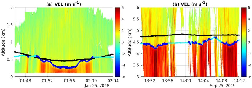
Remote Sens. 2021, 13, 1660                                                                                           2 of 17

                              velocity (VEL). However, for scientists using an automated as opposed to a purely visual
                              approach to radar data analysis, a quantitative estimate of the altitude of the melting layer
                              from radar data is highly desirable. Therefore, we developed software that detects and
                              flags the melting layer altitude in HCR data.
                                   Using radar data for melting layer detection, especially the polarimetric variables,
                              has proven very successful. Ground-based radars in the S-band [3,4], C-band [5], and
                              K-band [6] were successfully used for bright band and melting layer detection. Bright
                              band detection is also part of the convective/stratiform partitioning algorithms for the
                              space-borne Ka- and Ku-band radars of the Global Precipitation Measurement (GPM)
                              mission [7], and the W-band radar of the CloudSat mission [8].
                                   The primary goal of the proposed melting layer data product is to allow users to
                              distinguish easily between warm and cold clouds below and above the melting layer. It is
                              not aimed at studies of the melting layer itself and is not intended to distinguish between
                              the top and the bottom of the melting layer as is the case with other more specialized
                              algorithms, e.g., [9].
                                   In this study, we give a detailed description of the melting layer detection algorithm
                              and the resulting data product. The algorithm, as developed, was applied to HCR data from
                              three different field campaigns ranging in location from the tropics to the Southern Ocean
                              (see Section 2.1 for details). We analyze the results of the algorithm in a qualitative and
                              quantitative way and compare them to supplementary data sets. Noteworthy observations
                              of special melting layer features are highlighted and discussed.

                              2. Data
                              2.1. HCR Data
                                    HCR has been deployed in three major field campaigns. The Cloud Systems Evolution
                              in the Trades (CSET) project took place from 1 July to 12 August 2015, and consisted of 16
                              research flights (RFs) between California and Hawaii [10]. It was designed to describe and
                              explain the evolution of the boundary layer aerosol, cloud, and thermodynamic structures
                              within the north Pacific trade winds. The CSET HCR data are available at https://doi.
                              org/10.5065/D6CJ8BV7 [11]. The Southern Ocean Clouds, Radiation, Aerosol Transport
                              Experimental Study (SOCRATES) was conducted to further our understanding of clouds,
                              aerosols, air–sea exchanges, and their interactions over the Southern Ocean. The aircraft
                              was stationed in Hobart, Australia, and flew 15 RFs between 15 January and 24 February
                              2018 [12]. HCR SOCRATES data are available at https://doi.org/10.5065/D68914PH [13].
                              The third major field campaign for HCR was the Organization of Tropical East Pacific
                              Convection (OTREC) project, which aimed to determine the large-scale environmental
                              factors that control convection over tropical oceans. It took place in the Eastern Pacific and
                              extreme southwestern Caribbean and included 22 RFs between 7 August and 2 October
                              2019 [14]. OTREC HCR data are available at https://doi.org/10.26023/V9DJ-7T9J-PE0
                              S [15].
                                    HCR digitizes radar observations with a resolution of ~20 m in range and a temporal
                              resolution of 10 Hz, which at typical flight speeds yields a sample volume approximately
                              20 m long in the direction of flight. In addition to the Doppler radar fields, such as DBZ,
                              VEL, and LDR, reanalysis data from the ERA5 model, which have been interpolated to the
                              HCR time-range grid via linear interpolation in four dimensions (three space and the time
                              dimension), are also provided. For a detailed description of HCR data, data processing,
                              and quality control, see [2]. The variables used in the melting layer detection algorithm
                              are DBZ, LDR, VEL, spectrum width (WIDTH), and the FLAG field, which discriminates
                              between cloud echo and other echo types [2]. The 0 ◦ C isotherm of the interpolated ERA5
                              temperature field (TEMP) is used as a first estimate of the melting layer altitude and for
                              comparison with the resulting melting layer product. The dry-bulb temperature was chosen
                              as it is most readily available and most commonly used as alternative to melting layer
                              measurements. Analysis of the wet-bulb temperature, which may have better correlation
                              with the melting layer [16], is reserved for future studies.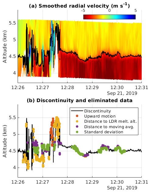
Remote Sens. 2021, 13, 1660                                                                                             3 of 17

                                    A special challenge when using high-frequency radars, such as HCR, as opposed to
                              S-band or C-band radars, comes from the fact that they are highly attenuated in liquid
                              precipitation [6]. In HCR data, areas where the radar signal is completely attenuated are
                              identified in the FLAG field. Fortunately, these areas rarely affect the melting layer detection
                              for reasons specific to the fact, that HCR is an airborne radar. When HCR operates in nadir-
                              pointing mode at high flight altitudes, the signal only travels through frozen precipitation,
                              which causes very little attenuation [17], until it encounters the melting layer. When the
                              aircraft flies below the melting layer, and HCR is in zenith-pointing mode, the radar is
                              generally in close proximity to the melting layer, as the aircraft needs to remain at a certain
                              altitude above ground. Again, the radar signal exhibits not enough attenuation to be
                              completely attenuated before it encounters the melting layer.

                              2.2. Dropsonde Data
                                   To compare the results of the melting layer detection algorithm with dropsonde data,
                              we use data from the Airborne Vertical Atmospheric Profiling System (AVAPS), which
                              measures high resolution vertical profiles of ambient temperature, pressure, humidity, wind
                              speed, and wind direction. AVAPS was also deployed on the HIAPER aircraft during all
                              three field campaigns. The data are available at https://doi.org/10.5065/D67H1GSR [18]
                              for CSET, https://doi.org/10.5065/D6QZ28SG [19] for SOCRATES, and https://doi.org/
                              10.26023/EHRT-TN96-9W04 [20] for OTREC [21].

                              3. Algorithm Description
                              3.1. Melting Layer Detection
                                    The melting of falling hydrometeors starts at the 0 ◦ C isotherm and continues on their
                              downward trajectory. Therefore, the melting layer is generally found at or below the 0 ◦ C
                              isotherm, hence the first step in the detection algorithm is to search for the 0 ◦ C isotherm
                              in the reanalysis TEMP field. It is important to recognize that there can be several 0 ◦ C
                              isotherms staggered on top of each other in cases of temperature inversions, and indeed
                              several such cases are observed in the SOCRATES data set (e.g., at 00:10 UTC in Figure 1a).
                              Therefore, in each ray, we first identify all pairs of gates where a change in the temperature
                              sign is observed. We then work along the time dimension to connect neighboring 0 ◦ C
                              isotherm gates horizontally to form continuous data periods (see Figure 1a for an example).
                              If several 0 ◦ C isotherm data periods are staggered on top of each other, each one is
                              processed separately in the steps that follow.
                                    To narrow the search area, we make an initial approximation of where we expect the
                              melting layer to be by simply applying an offset to the ERA5 0 ◦ C isotherm, so that the
                              approximate melting layer altitude is located just below the 0 ◦ C isotherm. The initial offset
                              value was ~200 m for SOCRATES and CSET and ~400 m for OTREC. The exact numbers
                              are not important as they are adjusted throughout the processing steps. For more details
                              on the offset between the model 0 ◦ C isotherm and the melting layer, see Section 4.2.
                                    The best HCR fields for our purpose are LDR, which shows a maximum at the melting
                              layer (Figure 1b), and VEL, which shows a discontinuity as hydrometeors increase their
                              fall speed when changing from the frozen to the liquid phase (Figure 1c). These two fields
                              stand out as prime candidates because they both show a strong signature at the melting
                              layer and have already been used by previous studies, e.g., [9,22]. Adding the DBZ field,
                              which sometimes shows a bright band signature at the melting layer altitude, did not yield
                              additional benefits. Both LDR and VEL are generally more sensitive to the melting of
                              hydrometeors, often showing characteristic signatures where no bright band is observed in
                              DBZ. Reflectivity was therefore not used in the algorithm.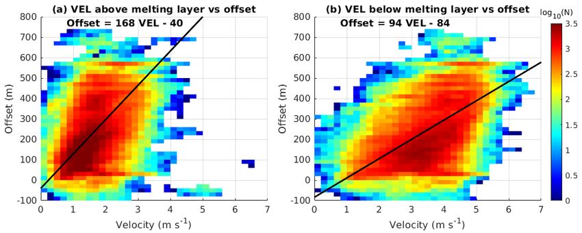
Remote Sens. 2021, 13, x FOR PEER REVIEW 4 of 19
Remote Sens. 2021, 13, 1660 4 of 17
Figure1.1.Input
Figure Inputvariables
variablesfor
forthe
themelting
melting layer
layer detection
detection algorithm:
algorithm: (a) ERA5 temperature
temperature (TEMP)
(TEMP)
with00◦ °C
with isotherm(black
C isotherm (blackline),
line), (b)
(b) linear
linear depolarization
depolarization ratio (LDR), and
and (c)
(c) radial
radial velocity
velocity(VEL,
(VEL,
positive values indicate downward motion). Times
positive values indicate downward motion). Times are in UTC.are in UTC.
We
Toneed
narrowto be
thecareful
searchtoarea,
remove artifacts
we make an that could
initial lead to erroneous
approximation results,
of where i.e., false
we expect the
detections. The biggest suspect in that regard is back-lobe echo, which
melting layer to be by simply applying an offset to the ERA5 0 °C isotherm, so that the occurs when HCR
isapproximate
pointing at the zenith,
melting andaltitude
layer the aircraft is flying
is located justnear
below thethe
ocean
0 °Cor land surface.
isotherm. In such
The initial off-
cases, the back
set value lobe m
was ~200 of for
the SOCRATES
radar is occasionally
and CSETreflected
and ~400offmthe forsurface
OTREC.and Thedetected
exact num-by
the
bersreceiver.
are notBack-lobe
importantecho is typically
as they characterized
are adjusted throughoutby a band of low reflectivity,
the processing steps. For highly
more
variable
details onradial velocity,
the offset and high
between spectrum
the model 0 °Cwidth.
isothermIt appears
and theatmelting
a radarlayer,
rangeseeequal to
Section
twice
4.2. the height of the aircraft above the surface, and it recedes and approaches in range as
the aircraft ascends
The best HCRor descends.
fields for ourApurpose
mechanismare to detect
LDR, whichthe back-lobe echo was developed
shows a maximum at the melt-
by [2], but because the LDR of the back-lobe echo strongly
ing layer (Figure 1b), and VEL, which shows a discontinuity as hydrometeors resembles the characteristics
increase
oftheir
the fall
melting
speedlayer,
whenthe thresholds
changing fromused
the by [2] were
frozen to thetightened
liquid phaseto remove
(Figurethe
1c).echo
These more
two
aggressively.
fields stand out We as
reject
primedatacandidates
where DBZ is lessthey
because thanboth −18 show
dBZ (as opposed
a strong to −20 at
signature dBZthe
inmelting
[2]) andlayer
WIDTH is greater than 1 m s −1 (1.4 m s−1 ). These new thresholds successfully
and have already been used by previous studies, e.g., [9,22]. Adding the
identified
DBZ field, thewhich
majority of the back-lobe
sometimes shows a echo,
brightexcept
band for a few cases
signature which
at the willlayer
melting be discussed
altitude,
indid
Section 3.5. In addition to removing the back-lobe echo,
not yield additional benefits. Both LDR and VEL are generally more sensitivewe remove all data that is
to the
identified as something other than cloud echo in the FLAG field, such as ocean or landRemote Sens. 2021, 13, 1660 5 of 17
surface echo, radar burst echo, etc. (see [2] for details). We also set thresholds on the LDR
data itself and use only data between −16 and −7 dB. Observations that are close to the
aircraft also proved to be unsuitable, and we removed all data within 150 m of the aircraft
in both the LDR and VEL fields.
After applying the quality checks described above, we search for a melting layer
signature in the LDR field. We constrain the search to within +/− 350 m, in range, from
the approximate altitude of the 0 ◦ C isotherm. The maximum LDR values detected within
this range indicate possible melting layer altitudes. Several checks of their validity are
performed. First, we calculate the 30 s moving average and moving standard deviation
in the time dimension. Detections for which the standard deviation exceeds 100 m are
removed because we do not expect the melting layer to vary significantly in altitude over
short distances. Then, we calculate the difference between the originally detected altitudes
and the moving average and remove those outliers where the difference exceeds 50 m.
Only those detections that pass these tests are retained as valid.
The next step is to adjust the model-approximated 0 ◦ C isotherms up or down to
match the results obtained from the LDR signature. We then search for a discontinuity
in the VEL field, within 960 m of the 0 ◦ C isotherm altitudes that were adjusted using
LDR. We smooth the VEL data in range using a 10-gate moving average, to reduce the
likelihood of identifying minor discontinuities. We then use the ischange MATLAB function
(https://www.mathworks.com/help/matlab/ref/ischange.html, accessed 28 April 2020),
which is based on [23], to identify the location of an abrupt change, i.e., a discontinuity in
VEL in the range direction. We interpret the altitude of the detected discontinuity as a proxy
for the melting layer altitude. The ischange function also provides the mean and variance of
the velocity above and below the melting layer. We use those in later processing steps.
An example of the detected velocity discontinuity is shown as the black line in Figure 2.
Once again, we verify these detections using a number of checks. A 100 s moving average is
computed in the time dimension. If the difference between the unsmoothed detections and
the moving average exceeds 100 m, the detection is discarded (purple dots in Figure 2b).
Similarly, the results are discarded if the 30 s moving standard deviation exceeds 35 m
(green dots). Results are also discarded if the difference between the LDR result and VEL
result exceeds 200 m (yellow dots). We also discard times where the mean VEL above
or below the melting layer indicates upward hydrometeor motion (red dots) because
this upward motion is only expected in updrafts that inhibit the formation of a readily
identifiable melting layer. In general, liquid hydrometeors below the melting layer exhibit
larger downward motion than frozen particles above the melting layer. Therefore, it is
reasonable to assume that the difference between the mean velocity above the melting layer
and the mean velocity below the melting layer must exceed a certain number, and indeed
it turns out that setting a threshold of 0.7 m s−1 is a good quality control step (not shown
in Figure 2b because no such cases were found in this specific example).
For the final melting layer altitude, we combine the LDR- and VEL-based estimates. If
the melting layer is detected in both the LDR and VEL fields, we use the LDR-based result.
Remaining outliers are removed by calculating the difference between the detected altitudes
and a 3 s moving average in time and excluding cases where the absolute difference exceeds
50 m. A 2 s moving average filter is applied. As a final quality control check, we exclude
results that lie more than 100 m above the model-derived 0 ◦ C isotherm as the model has
proven to be very accurate (see Section 4.2). It is important to note that the melting layer
altitudes detected in VEL are sometimes somewhat lower than those detected in LDR, as
has been observed in previous studies, e.g., [22], but the difference was not significant,
i.e., less than the overall noise, and therefore merging them into the same data field
seemed justified.it is reasonable to assume that the difference between the mean velocity above the melting
Remote Sens. 2021, 13, 1660 layer and the mean velocity below the melting layer must exceed a certain number, 6 ofand
17
indeed it turns out that setting a threshold of 0.7 m s−1 is a good quality control step (not
shown in Figure 2b because no such cases were found in this specific example).
Figure2.2.(a)
Figure (a)Smoothed
Smoothedradial
radialvelocity
velocity (color
(color shading) and detected discontinuity
discontinuity (black
(blackline).
line).(b)
(b)
Discontinuity(black
Discontinuity (blackline).
line).Color
Colordots
dotsindicate
indicateresults
resultsthat
thatwere
wereremoved
removedforforthe
thefollowing
followingreasons:
reasons:
red—upwardmotion
red—upward motionwas wasdetected;
detected;yellow—the
yellow—thedistance
distance to
to the
the melting
melting layer
layer altitude
altitude detected
detected inin
LDR exceeds 200 m; purple—the distance between the raw result and the 100 s movingaverage
LDR exceeds 200 m; purple—the distance between the raw result and the 100 s moving average
exceeds 100 m; green—the 30 s standard deviation exceeds 35 m. Times are in UTC.
exceeds 100 m; green—the 30 s standard deviation exceeds 35 m. Times are in UTC.
ItFor the final melting
is important to point layer altitude,
out that all thewe combine
constants andthe LDR- andused
thresholds VEL-based estimates.
in the processing
If thewere
steps melting layer ischosen
empirically detected in both
to work the LDR
for HCR 10 Hz and VEL
data andfields,
are notwe use thetoLDR-based
intended translate
toresult.
other Remaining outliers are
radar data without removed by
adjustments. In calculating
fact, when we thetried
difference between
to process HCRthe2 Hzdetected
data
altitudes and a 3 s moving average in time and excluding cases where
with the same algorithm, the results were not satisfactory. Instead, we decided to run the the absolute differ-
ence exceeds
algorithm at 1050Hzm.and
A 2interpolate
s moving average
the resultsfilter
tois2 applied.
Hz. As a final quality control check,
we exclude results that lie more than 100 m above the model-derived 0 °C isotherm as the
3.2. Melting
model has Layer
proven Interpolation
to be veryinaccurate
Time (see Section 4.2). It is important to note that the
melting layer altitudes
It is desirable to notdetected in VEL
only provide theare sometimes
users with thesomewhat
melting layerlower than those
altitude at timede-
tected
steps whenin LDR, as haslayer
a melting beenwas
observed in previous
identified in the LDR studies, e.g.,fields
or VEL [22], by
butthe
thealgorithm,
differencebut was
not to
also significant, i.e., less than
give an indication of itsthe overall
altitude whennoise, andno
either therefore
meltingmerging them into
layer signature the same
is detected
data field seemed justified.
or no clouds are observed at all. Of course, one may ask why we even provide melting
It is important
layer data where notocloudspoint out
are that all the constants
observed. and thresholds
We can envision severalused in the where
scenarios processing
an
steps weremelting
estimated empirically
layerchosen
might to workuseful
prove for HCReven 10outside
Hz dataofand are not
cloud intended
areas. to trans-
For example,
late to other
someone may radar
want to data without
combine HCRadjustments. In fact, when
data with satellite we triedand
observations to process
the HCRHCR 2 Hz
melting
layer estimate could be used for a satellite detected cloud in close proximity. We would also
like to point out that NCAR/EOL provides a combined data set that includes both HCR
and High Spectral Resolution Lidar (HSRL) data on the same grid. Having an estimate of
the melting layer altitude may prove useful in areas where HSRL observes clouds but HCR
does not (because of the different capabilities of the instruments).Remote Sens. 2021, 13, 1660 7 of 17
To fill in the missing time periods, we use different methods depending on the length
of the missing time interval. When a gap between two detected data points is shorter than
20 min, a simple linear interpolation between the detected data points is performed, and
we retain these interpolated points as a high-quality proxy for the actual melting layer
altitude. If the gap exceeds 20 min, we estimate the melting layer altitude by applying a
constant offset to the 0 ◦ C isotherm so that the estimated altitudes follow the 0 ◦ C isotherm.
To avoid jumps where the estimated altitudes join the detected altitudes, we define a
10 min transition period where a linear interpolation between the detected and estimated
altitudes is applied. Even though an interpolation is applied in the transition period, it is
still considered as part of the estimated data and not to be confused with the interpolated
points that fill the short gaps described above. The offset used for the estimated melting
layer is calculated in different ways for each field campaign. For SOCRATES and OTREC,
detected melting layer points were obtained in each flight. Therefore, the offset is calculated
as the mean offset over the respective flight. During CSET, cloud tops rarely exceeded the
altitude of the melting layer and, therefore, the melting layer could only be detected in
four flights. Calculating the offset on a flight by flight basis was therefore not possible and
we chose to use the mean offset calculated from the whole project (i.e., all four flights). A
detailed analysis of the offsets is presented in Section 4.2.
3.3. The Icing Level
For many applications, the actual altitude of the melting layer is not as important as
the question of whether a specific point in a cloud is located above or below the melting
layer, i.e., if it is part of a cold or warm cloud. Therefore, we would like to flag each 2D
(time range) data point as either warm or cold. However, before we can do that, we need to
decide how to handle situations where several melting layers are staggered on top of each
other (see Section 3.5). We clarify the meaning of “warm” and “cold” flags by introducing
the icing level. The American Meteorological Society [24] defines the icing level as the
“Lowest height above sea level at which an aircraft in flight may encounter icing” which
we interpret to coincide with the lowest melting layer found or estimated in HCR data.
3.4. The Melting Layer Product
The melting layer product comprises three temporal categories (Section 3.2): (1)
detections: times for which a melting layer altitude was actually detected in the LDR or VEL
field (dark blue in Figure 3); (2) interpolations: times with interpolated altitudes bridging
shorter gaps (light blue); (3) estimates: times with altitudes estimated from the 0 ◦ C isotherm
with an appropriate offset (green). We flag each separately. We also indicate whether the
melting layer coincides with the icing level (i.e., whether it is the lowest melting layer) or if
it is above the icing level, and we flag the icing level itself (red). In addition, we flag the
0 ◦ C isotherm for the users’ convenience (black), again indicating whether it is above or
below the icing level. Data points that are not flagged as a melting layer point are flagged
as being either in the warm (below the icing level, pink in Figure 3b) or cold (above the
icing level, yellow in Figure 3b) region. The actual flag values are stored in the metadata of
the distributed CfRadial NetCDF files. The altitude of the icing level is provided as a 1D
(time dimension) data field.
3.5. Product Quality Assessment
When developing algorithms for product creation, it is often relatively easy to write
code that gives the desired results for a few selected cases. The real challenge is to de-
velop an algorithm that is robust enough to handle at least the majority of highly diverse
conditions. Tuning an algorithm for conditions as different as, for example, OTREC and
SOCRATES, inevitably requires some compromise and finding the right balance between
missed detections and false positives. We decided to err on the side of missing some
detections because we believe that the interpolations, and, to a lesser degree, the estimates,
can serve as a high-quality substitute when detections are missed. An example in whichshorter gaps (light blue); (3) estimates: times with altitudes estimated from the 0 °C iso-
therm with an appropriate offset (green). We flag each separately. We also indicate
whether the melting layer coincides with the icing level (i.e., whether it is the lowest melt-
ing layer) or if it is above the icing level, and we flag the icing level itself (red). In addition,
Remote Sens. 2021, 13, 1660 we flag the 0 °C isotherm for the users’ convenience (black), again indicating whether it 8isof 17
above or below the icing level. Data points that are not flagged as a melting layer point
are flagged as being either in the warm (below the icing level, pink in Figure 3b) or cold
(above the icing level, yellow in Figure 3b) region. The actual flag values are stored in the
short time periods are easily assessed visually but missed by the algorithm is shown in
metadata of the distributed CfRadial NetCDF files. The altitude of the icing level is pro-
Figure
vided as3 at 17:28
a 1D (timeUTC.
dimension) data field.
Figure 3. Example
Figure Exampleofof thethe
melting layer
melting product:
layer (a) radial
product: velocityvelocity
(a) radial and (b) and
melting
(b) layer fieldlayer field
melting
where yellow (pink) indicates data above (below) the icing level (red line). Detections
where yellow (pink) indicates data above (below) the icing level (red line). Detections (dark(dark blue),blue),
interpolations (light blue), and estimates (green) are marked with dots. Times are in UTC.
interpolations (light blue), and estimates (green) are marked with dots. Times are in UTC.
3.5. Product Quality Assessment
As the melting layer is relatively easy to identify visually in the radar fields, the most
straightforward
When developingway toalgorithms
evaluate the accuracycreation,
for product of the algorithm is to examine
it is often relatively easy to the results
write
code thatTo
visually. gives the desired
do this, results
we plotted thefor a few in
results selected
hourlycases. The realwhich
increments, challenge
wereis to develop
then carefully
an algorithm
screened for that
bothismissed
robust enough
events to handle
and falseatdetections.
least the majority
From of thehighly diverse
visual condi- we
inspection,
tions. Tuning an algorithm for conditions as different
concluded that, overall, the algorithm performs very well. as, for example, OTREC and SOC-
RATES, inevitably requires some compromise and finding the right balance between
Even if the melting layer is detected in the correct gates, in principle there could still be
missed
an error detections and false
in the melting layerpositives.
altitude ifWethedecided to err is
gate altitude onincorrect.
the side ofHCRmissing
gate some de- are
altitudes
tections from
derived because we believe
a global that thesystem
positioning interpolations,
(GPS) and and, to a lesser
inertial degree,system
navigation the estimates,
(INS) unit,
can serve
which as a high-quality
is mounted substitute
in the nose when pod.
of the radar detections are missed.
The GPS/INS An example
altitudes in which for
are corrected
short time periods
gravitational effectsare easily
on the assessed
Earth’s visually
surface usingbut
the missed by the algorithm
Earth Gravitation Modelis shown in see
(EGM2008,
Figure 3 at 17:28 UTC.
https://earth-info.nga.mil/GandG/wgs84/gravitymod/egm2008/, accessed 8 December
2019). The altitudes can easily be verified by comparing the gate altitude of the ocean’s
surface with the GPS/INS altitude. Such a comparison was carried out for all three field
campaigns (not shown) and shows agreement within +/− 20 m, which also happens to
be the gate spacing of HCR. We therefore conclude that accurately detected melting layer
altitudes have an uncertainty of ~20 m.
The algorithm was originally developed for the OTREC data set, which has many
suitable clouds with clear melting layer structures. Generalizing the algorithm to work well
for CSET but especially SOCRATES proved more complicated. During SOCRATES, flight
plans were designed to zigzag vertically through the near-surface cloud layer, which often
coincided with the melting layer altitude, leading to multiple melting layer crossings by the
aircraft. During these zigzag maneuvers, HCR pointing regularly switched between zenith
and nadir, which led to additional difficulties for the algorithm. An example of a situationRemote Sens. 2021, 13, 1660 9 of 17
where the identification of the icing level is not straightforward is shown in Figure 4a.
Remote Sens. 2021, 13, x FOR PEERAnother
REVIEW challenge came from the fact that during the southernmost parts of the 10
SOCRATES
of 19
flights, air temperature often dropped below 0 ◦ C at the surface so the intersection of the
melting layer with the surface needed to be handled appropriately (Figure 4b).
FigureFigure 4. Melting
4. Melting layerlayer product
product forfor
(a)(a) a situationwhere
a situation where the
the flight
flightpattern
patternintersects
intersectsseveral melting
several layers,
melting (b) a situation
layers, (b) a situation
where the melting layer intersects the surface. (c,d) LDR and the melting layer data product for a case where the back-lobe
wherefilter
the melting layer intersects the surface. (c,d) LDR and the melting layer data product for a case where the back-lobe
did not capture all of the back-lobe data (see text for details). Colors in (a,b,d) as in Figure 3b. Times are in UTC.
filter did not capture all of the back-lobe data (see text for details). Colors in (a,b,d) as in Figure 3b. Times are in UTC.
During SOCRATES, we found several cases in which the back-lobe echo was not
Duringfiltered
properly SOCRATES, we found
and removed several
(Section 3.1),cases in which
leading to falsethe back-lobe
positive echo was
detections not prop-
(Figure
erly filtered
4c,d). and removed
Fortunately, (Section
these cases proved3.1),
rare,leading
and were tounique
false positive detections
to SOCRATES. We must(Figure
also 4c,d).
Fortunately,
point out that these
the cases proved
algorithm was rare, and were
developed unique
for zenith andto SOCRATES.operations
nadir-pointing We must onlyalso point
outand thatis,the algorithm
therefore, was developed
unreliable for zenith
during sea surface and nadir-pointing
calibration operations
events during which only and
the radar
is, istherefore,
scanning 20° off nadirduring
unreliable perpendicular to thecalibration
sea surface aircraft for several
eventsminutes
during for reflectivity
which the radar is
calibration
scanning 20◦monitoring
off nadir purposes [2]. As to
perpendicular seathe
surface calibration
aircraft eventsminutes
for several are generally per-
for reflectivity
formed in clear air conditions, this problem has little relevance. In addition,
calibration monitoring purposes [2]. As sea surface calibration events are generally per- the algorithm
is designed
formed in clearto detect a single melting
air conditions, layer in the
this problem hasvicinity of the model
little relevance. 0 °C isotherm
In addition, the and,
algorithm
therefore, does not properly handle cases in which the melting layer splits into two (see
is designed to detect a single melting layer in the vicinity of the model 0 ◦ C isotherm and,
Section 4.1 below). In these situations, it tends to jump from one to the other, or misses
therefore, does not properly handle cases in which the melting layer splits into two (see
both.
Section 4.1 below). In these situations, it tends to jump from one to the other, or misses both.
4. Discussion of the Identified Melting Layer
4. Discussion of the Identified Melting Layer
4.1. Special Observations
4.1. Special Observations
It is expected but nonetheless interesting to observe how strongly the melting layer
It is expected
altitude but
varies, even nonetheless
within interesting
an individual to observe
cloud. This howtrue
is especially strongly theofmelting
in regions strong layer
altitude varies,
convection evenareas
where within
withanstrong
individual
meltingcloud. This is especially
layer signatures true inby
are interrupted regions of strong
updrafts.
convection
An example where areas
of such with is
a region strong
shown melting layer
in Figure signatures
5a, where are interrupted
the melting layer on onebyside
updrafts.
Anofexample
an updraft of region
such a(~12:27
regionUTC)is shown
is 200inmFigure
higher 5a,
thanwhere
on thethe melting
other side oflayer on one side
the updraft
of region (~12:29
an updraft UTC).(~12:27
region Even inUTC)regionsis where
200 m the melting
higher thanlayer is not
on the interrupted
other by an
side of the updraft
updraft,
region we sometimes
(~12:29 UTC). Evenobserve strong variability
in regions where the in the melting
melting layerisaltitude
layer (Figure 5b) by an
not interrupted
updraft, we sometimes observe strong variability in the melting layer altitude (Figure 5b)Remote Sens. 2021, 13, 1660 10 of 17
or even jumps (just after 16:18 UTC, Figure 5c) as the melting layer is modified by storm
internal processes.
We also observe several cases where the melting layer altitude is lower in the center
of a cloud feature (01:55 UTC, Figure 6a; 13:53 UTC and 14:10 UTC, Figure 6b) in areas of
increased fall speeds. We speculate that the melting layer is either pushed lower in the
center of a strong downdraft as cold air is transported downward or it only appears lower
as larger particles with higher fall speeds take longer to melt and therefore stay frozen
to lower altitudes. An analysis of the connection between particle fall speed and vertical
offset between the 0 ◦ C isotherm and the melting layer is presented in Section 4.2.
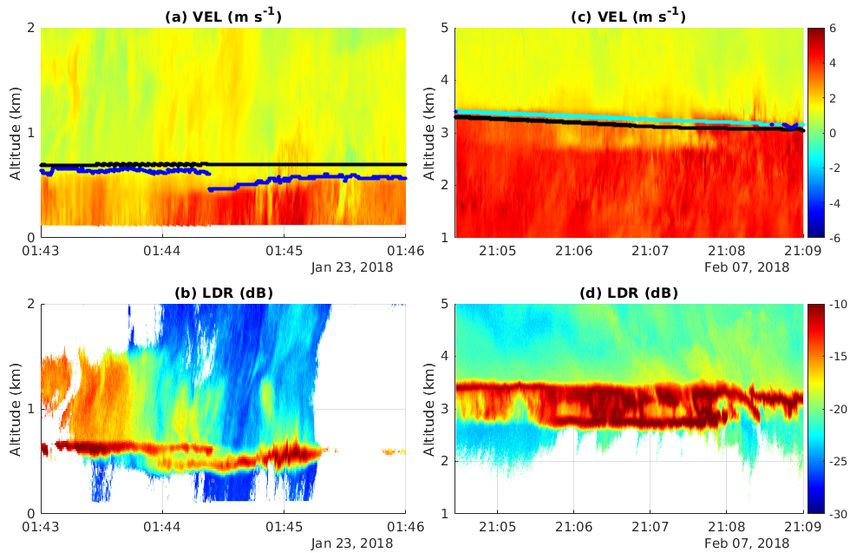
Of special interest are regions with what we refer to as split melting layers, where two
vertically staggered melting layer signatures are observed in the VEL and LDR fields in very
close proximity to each other (Figure 7). Note that this phenomenon indicates a splitting of
one distinct melting layer and is not to be confused with cases of several staggered melting
layers caused by temperature inversions (Section 3.5). The split melting layer phenomenon
was also recently observed and described by [22] and was attributed to the melting of two
distinct populations of ice particles. The fact that we observed split melting layers over the
Southern Ocean during the SOCRATES field campaign (Figure 7) confirms
Remote Sens. 2021, 13, x FOR PEER REVIEW
that the authors
12 of 19
of [22] were correct to conclude that “more reports of this phenomenon are expected in
the future”.
Figure 5.5.Radial
Figure Radial velocity (color(color
velocity shading) and melting
shading) andlayer detections
melting layer(dark blue), interpolations
detections (dark blue), interpolations
(light blue), estimates (green), and model 0 °C isotherm
◦ (black) for examples of strong variability
(light blue), estimates (green), and model 0 C isotherm (black) for examples of strong variability of
of the melting layer within short time periods, collected in 2019 during OTREC on (a) September
the melting
21, (b) Augustlayer within
16, and short25.
(c) August time periods,
Times collected in 2019 during OTREC on (a) September 21, (b)
are in UTC.
August 16, and (c) August 25. Times are in UTC.Figure 5. Radial velocity (color shading) and melting layer detections (dark blue), interpolations
Remote Sens. 2021, 13, 1660 11 of 17
(light blue), estimates (green), and model 0 °C isotherm (black) for examples of strong variability
of the melting layer within short time periods, collected in 2019 during OTREC on (a) September
21, (b) August 16, and (c) August 25. Times are in UTC.
Remote Sens. 2021, 13, x FOR PEER REVIEW 13 of 19
Figure 6. Radial velocity and melting layer data for examples where the melting layer is lowered towards the center of
Figure 6. Radial velocity and melting layer data for examples where the melting layer is lowered towards the center of
storms, collected during (a) SOCRATES and (b) OTREC. Colors as in Figure 5. Times are in UTC.
storms, collected during (a) SOCRATES and (b) OTREC. Colors as in Figure 5. Times are in UTC.
Figure 7.
Figure 7. Radial
Radial velocity
velocity and
and melting
melting layer
layer data
data (a,c) and linear
(a,c) and linear depolarization
depolarization ratio
ratio (b,d)
(b,d) for two cases
for two cases (left
(left panels
panels and
and
right panels) where a split melting layer was observed. Colors in (a,c) as in Figure 5. Times are in UTC.
right panels) where a split melting layer was observed. Colors in (a,c) as in Figure 5. Times are in UTC.
4.2. Offset between the Melting Layer and the 0 °C Isotherm
In Section 4.1, we have shown that the altitude of the melting layer not only depends
on the properties of the particles, such as their type or size, and external factors, such as
temperature gradient and air motion, but is also determined by cloud physical and dy-
namical processes.
One factor that seems of particular importance in determining the vertical offset be-
tween the 0 °C isotherm and the melting layer is the fall speed of the particles. To investi-
gate its role, the mean radial velocity of the ten gates above and ten gates below each
melting layer detection is computed and compared with the vertical offset at that specific
time (Figure 8). Both the velocity above (Figure 8a) and below the melting layer (Figure
8b) show a clear correlation with the offset. A geometric mean regression [25] is performedRemote Sens. 2021, 13, 1660 12 of 17
4.2. Offset between the Melting Layer and the 0 ◦ C Isotherm
In Section 4.1, we have shown that the altitude of the melting layer not only depends
on the properties of the particles, such as their type or size, and external factors, such
as temperature gradient and air motion, but is also determined by cloud physical and
dynamical processes.
One factor that seems of particular importance in determining the vertical offset
between the 0 ◦ C isotherm and the melting layer is the fall speed of the particles. To
investigate its role, the mean radial velocity of the ten gates above and ten gates below
each melting layer detection is computed and compared with the vertical offset at that
specific time (Figure 8). Both the velocity above (Figure 8a) and below the melting layer
(Figure 8b) show a clear correlation with the offset. A geometric mean regression [25] is
performed between the offset and velocity points, and the resulting regression lines and
coefficients are shown in Figure 8. The slope of the regression line is steeper for velocities
above the melting layer as fall speeds are smaller in the frozen region. The correlation
Remote Sens. 2021, 13, x FOR PEER REVIEW 14 of 19
between velocity and offset suggests that velocity either above or below the melting layer
◦
can potentially be used to estimate the altitude of the melting layer from the 0 C isotherm
in datasets where no melting layer altitude is provided.
Figure
Figure8.8.Scatter
Scatterplot
plotof
of10
10 gate
gate mean
mean radial
radial velocity above (a)
velocity above (a) and
and below
below(b)(b)the
themelting
meltinglayer
layervs.
vs.offset
offsetbetween
betweenthe
the0 0◦ C°C
isotherm
isothermandandthe
themelting
melting layer
layer with
with geometric
geometric regression line (black).
regression line (black). Color
Color shading
shadingshows
showsthe
thenumber
numberofofdata
datapoints
pointsinin
logarithmic units.
logarithmic units.
Due
Due toto the
the many factors influencing
many factors influencing the the offset
offset between
betweenthe the00◦ C
°Cisotherm
isothermand andthethe
melting
melting layer,
layer, especially the fall
especially the fall speed
speed of
of the
theparticles,
particles,ititisisnot
notsurprising
surprisingthat
thatthe
thedistance
distance
between
between the
the detected
detected melting layer
layer and the 00 ◦°C
and the isotherm varies
C isotherm varies between
betweenfield
fieldcampaigns,
campaigns,
between
between individual
individual flights
flights of a specific
specific field
field campaign,
campaign, and andalso
alsowithin
withineach
eachflight
flightand
and
indeed
indeed within
within each
each cloud. These variations are generally
generally on onthe
theorder
orderofofaafew
fewhundred
hundred
meters. Mean
meters. Mean offsets between the 0 ◦°C
offsets between C isotherm,
isotherm, which
which isisgenerally
generallyvery
veryaccurate
accurate(see(see
below), and
below), and the
the melting layer per flight
flight and
and perperfield
fieldcampaign
campaignare areshown
shownininTable
Table1.1.
Table 1. Offset (in m) between the 0 °C isotherm and the detected melting layer for all three field
campaigns. Positive offsets indicate that the melting layer was located below the 0 °C isotherm.
CSET SOCRATES OTREC
(m) (m) (m)
Mean 169.83 156.44 322.91
St Dev 138.98 52.63 115.00
RF01 326.15 140.52 248.44
RF02 115.10 441.43
RF03 19.19 115.13 383.69Remote Sens. 2021, 13, 1660 13 of 17
Table 1. Offset (in m) between the 0 ◦ C isotherm and the detected melting layer for all three field
campaigns. Positive offsets indicate that the melting layer was located below the 0 ◦ C isotherm.
CSET SOCRATES OTREC
(m) (m) (m)
Mean 169.83 156.44 322.91
St Dev 138.98 52.63 115.00
RF01 326.15 140.52 248.44
RF02 115.10 441.43
RF03 19.19 115.13 383.69
RF04 172.68 134.93
RF05 110.60 95.91
RF06 134.09 326.40
RF07 249.11
RF08 210.99 383.64
RF09 76.73 364.44
RF10 213.33 518.08
RF11 211.04 345.36
RF12 93.50 194.66 190.12
RF13 152.76 364.60
RF14 76.67 192.24
RF15 173.20 288.07
RF16 240.48 383.75
RF17 364.65
RF18 364.45
RF19 172.71
RF20 489.71
RF21 440.80
RF22 287.79
The offset in OTREC is, on average, 323 m and twice as big as the 156 m offset observed
in SOCRATES. We speculate that this difference is the result of the very different types of
cloud observed during these two field campaigns. The tropical convective systems sampled
during OTREC likely contain larger particles with higher fall speeds than the shallow cloud
layers observed in SOCRATES. Clouds sampled in CSET were also mostly shallow in
nature, which may explain the smaller offset of 170 m; however, because of the limited
number of detections and the large variability, we cannot draw definitive conclusions for
CSET. It is remarkable that individual flights in OTREC show offsets of up to, and in one
case (RF10) even above, 500 m, which underlines the importance of using the melting layer,
as opposed to the model temperature, to delineate warm from cold clouds.
The offsets listed in Table 1 and the conclusions derived from them depend on the
accuracy of the ERA5 temperature data, specifically the altitude of the 0 ◦ C isotherm. To
assess the quality of the 0 ◦ C isotherm model data, we compare them with temperature
data from dropsondes that were launched from HIAPER during all three field campaigns.
For each dropsonde profile, we find all altitudes where a change in sign is reported, identify
the one that is closest to the 0 ◦ C isotherm in the ERA5 data, and calculate the difference
between the two. It is important to use the 0 ◦ C point that is closest to the melting layer
because the dropsonde data shows even more structure in the temperature profile than the
model data, as expected (Figure 9).
Overall, the comparisons for all three field campaigns show excellent agreement
between the dropsonde and ERA5 0 ◦ C levels (Figure 10). The mean altitude difference
between the two is 78 m for CSET, 32 m for SOCRATES, and 27 m for OTREC. The better
agreement for SOCRATES and OTREC is likely due to the fact that the dropsonde data
was assimilated into the ERA5 model for these two field campaigns, but not for CSET. It
is interesting to note that in all three field campaigns the dropsonde 0 ◦ C isotherm was
observed slightly above the ERA5 0 ◦ C isotherm, which means that the model is generally
reporting slightly lower temperatures than the dropsondes. From the slightly negative biasRemote Sens. 2021, 13, 1660 14 of 17
in the model, one would expect the actual offset between the melting layer and the 0 ◦ C
isotherm to be slightly larger than that reported in Table 1. To confirm this assumption, we
calculate the offset using dropsonde data. We distinguish between offsets calculated with
detected, interpolated, and estimated melting layer altitudes. Indeed, the offset calculated
from dropsonde data is, at just more than 200 m, slightly larger than the 156 m calculated
from ERA5 temperatures (Table 1) for SOCRATES. For OTREC, which has not only the
Remote Sens. 2021, 13, x FOR PEER REVIEW
smallest temperature bias between the dropsondes and the ERA5 data but also the largest
variability in the offset calculation, there is no significant difference between the offsets
calculated with dropsonde vs. ERA5 temperatures.
Figure 9.9.Example
Figure Example comparing
comparing melting layer layer
melting (colors(colors
as in Figure
as in5)Figure
and ERA5 temperature
5) and with
ERA5 temperature
dropsonde temperatures. Vertical columns show dropsonde temperatures with the
dropsonde temperatures. Vertical columns show dropsonde temperatures with black dots within black dots
vertical columns indicating 0 ◦ C data points. Background fields are (a) radial velocity and (b) ERA5
the vertical columns indicating 0 °C data points. Background fields are (a) radial velocity a
temperatures. Times are in UTC.
ERA5 temperatures. Times are in UTC.Remote Sens. 2021, 13, x FOR PEER REVIEW 17 of 1
Remote Sens. 2021, 13, 1660 15 of 17
Figure10.
Figure 10.HCR
HCRidentified
identifiedmelting
melting layer altitude
layer vs. vs.
altitude dropsonde
dropsonde 0 ◦ C0 isotherm for the
°C isotherm for(a)
theCSET,
(a) CSET, (b)
SOCRATES,
(b) SOCRATES,and and(c)
(c)OTREC
OTREC field campaigns.Shown
field campaigns. Shownare are comparisons
comparisons of detected
of detected (dark(dark
blue),blue), in-
terpolated (light
interpolated (lightblue),
blue),estimated
estimated (green)
(green) melting
melting layer,layer, 0 ◦ C isotherm
and ERA5
and ERA5 0 °C isotherm (black)
(black) data. Thedata. The
identityline
identity line is shown
is shown in red.
in red. Offsets
Offsets and standard
and standard deviations
deviations areinlisted
are listed in the
the upper leftupper left corners.
corners.
5. Conclusions
5. Conclusions
We developed a melting layer detection algorithm for HCR data. The algorithm uses
the LDRWeand
developed
VEL fieldsa from
melting layer detection
the radar. algorithm
The final product for HCR
combines data. The
confirmed algorithm use
detections,
the LDR
values and VEL in
interpolated fields
timefrom the radar.
between Theevents,
detection final product combines
and estimated confirmed
values where nodetection
values interpolated
detections are availableinintime
closebetween detection
time proximity. ERA5 ◦
events, and estimated
0 C isotherm values
values are where no de
provided
as well. The
tections are icing level in
available is defined
close timeas the lowest melting
proximity. ERA5 0layer in each vertical
°C isotherm valuesray,
areand
provided a
data points are flagged as above or below the icing level so that it is
well. The icing level is defined as the lowest melting layer in each vertical ray,easy for the users to and dat
determine whether a specific location is in the warm or cold region of the atmosphere.
points are flagged as above or below the icing level so that it is easy for the users to deter The
algorithm was applied to observations from three fundamentally different field campaigns;
mine whether a specific location is in the warm or cold region of the atmosphere. Th
algorithm was applied to observations from three fundamentally different field cam
paigns; the results were carefully checked for accuracy and found to be very reliable. A
the algorithm shows excellent capabilities in both tropical regions and at high latitudeRemote Sens. 2021, 13, 1660 16 of 17
the results were carefully checked for accuracy and found to be very reliable. As the
algorithm shows excellent capabilities in both tropical regions and at high latitudes, we are
confident that it will translate to other regions of the world without major adjustments.
The melting layer is highly variable on very short scales and strongly modified by
storm internal processes. We found cases with sudden jumps in the melting layer altitude,
wave-like structures within single storms, and strong altitude differences on opposite sides
of updraft regions. The melting layer sometimes has a tendency to be lower towards the
middle of cloud features with strong downdrafts. In some cases, the melting layer splits
into two horizontal layers.
The magnitude of the downward offset of the melting layer from the model 0 ◦ C
isotherm depends on the type of storm sampled. In tropical storms, as sampled in the
OTREC field campaign, it can exceed 500 m, while in regions with shallow clouds, such
as those observed during SOCRATES and CSET, it tends to be less than a few hundred
meters. The offset calculations were verified with dropsonde data, which show excellent
agreement with the ERA5 model. A relationship between the offset and the particle fall
speed both above and below the melting layer could be established. As expected, velocities
in the frozen region above the melting layer were generally smaller than those in the liquid
region below the melting layer, which resulted in a steeper regression line in the frozen
compared to the liquid region.
Funding: This material is based upon work supported by the National Center for Atmospheric
Research, which is a major facility sponsored by the National Science Foundation under Cooperative
Agreement No. 1852977.
Data Availability Statement: HCR data are available at https://doi.org/10.5065/D6CJ8BV7 [11]
(CSET), https://doi.org/10.5065/D68914PH [13] (SOCRATES), and https://doi.org/10.26023/V9
DJ-7T9J-PE0S [15] (OTREC). AVAPS data are available at https://doi.org/10.5065/D67H1GSR [18]
(CSET), https://doi.org/10.5065/D6QZ28SG [19] (SOCRATES), and https://doi.org/10.26023/EHRT-
TN96-9W04 [20] (OTREC).
Acknowledgments: I would like to thank Mike Dixon and Holger Vömel for helpful discussions
and comments.
Conflicts of Interest: The author declares no conflict of interest. The funders had no role in the design
of the study; in the collection, analyses, or interpretation of data; in the writing of the manuscript, or
in the decision to publish the results.
References
1. Vivekanandan, J.; Ellis, S.; Tsai, P.; Loew, E.; Lee, W.-C.; Emmett, J.; Dixon, M.; Burghart, C.; Rauenbuehler, S. A Wing Pod-Based
Millimeter Wavelength Airborne Cloud Radar. Geosci. Instrum. Methods Data Syst. 2015, 4, 161–176. [CrossRef]
2. Romatschke, U.; Dixon, M.; Tsai, P.; Loew, E.; Vivekanandan, J.; Emmett, J.; Rilling, R. The NCAR Airborne 94-GHz Cloud Radar:
Calibration and Data Processing. arXiv 2021. [CrossRef]
3. Brandes, E.A.; Ikeda, K. Freezing-Level Estimation with Polarimetric Radar. J. Appl. Meteorol. Climatol. 2004, 43, 1541–1553.
[CrossRef]
4. Lee, J.-E.; Jung, S.-H.; Kwon, S. Characteristics of the Bright Band Based on Quasi-Vertical Profiles of Polarimetric Observations
from an S-Band Weather Radar Network. Remote Sens. 2020, 12, 4061. [CrossRef]
5. Sanchez-Rivas, D.; Rico-Ramirez, M.A. Detection of the Melting Level with Polarimetric Weather Radar. Atmos. Meas. Tech. 2021,
14, 2873–2890. [CrossRef]
6. Massmann, A.K.; Minder, J.R.; Garreaud, R.D.; Kingsmill, D.E.; Valenzuela, R.A.; Montecinos, A.; Fults, S.L.; Snider, J.R. The
Chilean Coastal Orographic Precipitation Experiment: Observing the Influence of Microphysical Rain Regimes on Coastal
Orographic Precipitation. J. Hydrometeorol. 2017, 18, 2723–2743. [CrossRef]
7. Awaka, J.; Le, M.; Chandrasekar, V.; Yoshida, N.; Higashiuwatoko, T.; Kubota, T.; Iguchi, T. Rain Type Classification Algorithm
Module for GPM Dual-Frequency Precipitation Radar. J. Atmos. Ocean. Technol. 2016, 33, 1887–1898. [CrossRef]
8. Haynes, J.M. CloudSat 2C-PRECIP-COLUMN Data Product Process Description and Interface Control Document. Available
online: http://www.cloudsat.cira.colostate.edu/sites/default/files/products/files/2C-PRECIP-COLUMN_PDICD.P1_R05.
rev1_pdf (accessed on 21 April 2021).
9. Le, M.; Chandrasekar, V. Hydrometeor Profile Characterization Method for Dual-Frequency Precipitation Radar Onboard the
GPM. IEEE Trans. Geosci. Remote Sens. 2013, 51, 3648–3658. [CrossRef]Remote Sens. 2021, 13, 1660 17 of 17
10. Albrecht, B.; Ghate, V.; Mohrmann, J.; Wood, R.; Zuidema, P.; Bretherton, C.; Schwartz, C.; Eloranta, E.; Glienke, S.; Donaher, S.;
et al. Cloud System Evolution in the Trades—CSET. Bull. Am. Meteorol. Soc. 2019, 100, 93–121. [CrossRef] [PubMed]
11. NCAR/EOL Remote Sensing Facility. CSET: NCAR HCR Radar Moments Data. Version 2.1; UCAR/NCAR-Earth Observing
Laboratory: Boulder, CO, USA, 2021.
12. McFarquhar, G.M.; Bretherton, C.; Marchand, R.; Protat, A.; DeMott, P.J.; Alexander, S.P.; Roberts, G.C.; Twohy, C.H.; Toohey, D.;
Siems, S.; et al. Observations of Clouds, Aerosols, Precipitation, and Surface Radiation over the Southern Ocean: An Overview of
CAPRICORN, MARCUS, MICRE and SOCRATES. Bull. Am. Meteorol. Soc. 2020, 1, 1–92. [CrossRef]
13. NCAR/EOL Remote Sensing Facility. SOCRATES: NCAR HCR Radar Moments Data. Version 2.1; UCAR/NCAR-Earth Observing
Laboratory: Boulder, CO, USA, 2021.
14. Fuchs-Stone, Ž.; Raymond, D.J.; Sentić, S. OTREC2019: Convection Over the East Pacific and Southwest Caribbean. Geophys. Res.
Lett. 2020, 47, e2020GL087564. [CrossRef]
15. NCAR/EOL Remote Sensing Facility. OTREC: NCAR HCR Radar Moments Data. Version 2.2; UCAR/NCAR-Earth Observing
Laboratory: Boulder, CO, USA, 2021.
16. Allabakash, S.; Lim, S.; Jang, B.-J. Melting Layer Detection and Characterization Based on Range Height Indicator–Quasi Vertical
Profiles. Remote Sens. 2019, 11, 2848. [CrossRef]
17. Li, L.; Sekelsky, S.M.; Reising, S.C.; Swift, C.T.; Durden, S.L.; Sadowy, G.A.; Dinardo, S.J.; Li, F.K.; Huffman, A.; Stephens, G.; et al.
Retrieval of Atmospheric Attenuation Using Combined Ground-Based and Airborne 95-GHz Cloud Radar Measurements. J.
Atmospheric Ocean. Technol. 2001, 18, 1345–1353. [CrossRef]
18. UCAR/NCAR-Earth Observing Laboratory. NSF/NCAR GV (HIAPER) QC Dropsonde Data. Version 4.0; UCAR/NCAR-Earth
Observing Laboratory: Boulder, CO, USA, 2016.
19. UCAR/NCAR-Earth Observing Laboratory; Voemel, H. NCAR/EOL Quality Controlled Dropsonde Data. Version 1.1; UCAR/NCAR-
Earth Observing Laboratory: Boulder, CO, USA, 2018.
20. UCAR/NCAR-Earth Observing Laboratory; Voemel, H. NCAR/EOL AVAPS Dropsonde QC Data. Version 1.0; UCAR/NCAR-Earth
Observing Laboratory: Boulder, CO, USA, 2019.
21. Vömel, H.; Goodstein, M.; Tudor, L.; Witte, J.; Fuchs-Stone, Ž.; Sentić, S.; Raymond, D.; Martinez-Claros, J.; Juračić, A.; Maithel, V.;
et al. High-Resolution in Situ Observations of Atmospheric Thermodynamics Using Dropsondes during the Organization of
Tropical East Pacific Convection (OTREC) Field Campaign. Earth Syst. Sci. Data Discuss. 2021, 17, 1107–1117. [CrossRef]
22. Li, H.; Moisseev, D. Two Layers of Melting Ice Particles Within a Single Radar Bright Band: Interpretation and Implications.
Geophys. Res. Lett. 2020, 47, e2020GL087499. [CrossRef]
23. Killick, R.; Fearnhead, P.; Eckley, I.A. Optimal Detection of Changepoints With a Linear Computational Cost. J. Am. Stat. Assoc.
2012, 107, 1590–1598. [CrossRef]
24. American Meteorological Society Icing Level-Glossary of Meteorology. Available online: https://glossary.ametsoc.org/wiki/
Icing_level (accessed on 9 March 2021).
25. Trujillo-Ortiz, A. Gmregress. MATLAB Central File Exchange 2018. Available online: https://www.mathworks.com/matlabcentral/
fileexchange/27918-gmregress (accessed on 18 March 2018).You can also read


