A workflow for seismic imaging with quantified uncertainty
←
→
Page content transcription
If your browser does not render page correctly, please read the page content below
A workflow for seismic imaging with quantified uncertainty

                                                   Carlos H. S. Barbosaa,b,1 , Liliane N. O. Kunstmannd,2 , Rômulo M. Silvaa,b,3 , Charlan D. S. Alvesa,4 ,
                                                   Bruno S. Silvab,5 , Djalma M. S. Filhoe,6 , Marta Mattosod,7 , Fernando A. Rochinhac,1 , Alvaro L.G.A.
                                                                                                Coutinhoa,7,∗
                                                               a High-Performance Computing Center, COPPE, Federal University of Rio de Janeiro, Brazil
                                                                  b Departmentof Civil Engineering, COPPE, Federal University of Rio de Janeiro, Brazil
                                                              c Department of Mechanical Engineering, COPPE, Federal University of Rio de Janeiro, Brazil
                                                                 d Department of Computer Science, COPPE, Federal University of Rio de Janeiro, Brazil
                                                                                                  e CENPES, Petrobras
arXiv:2001.06444v1 [physics.geo-ph] 17 Jan 2020

                                                  Abstract

                                                  The interpretation of seismic images faces challenges due to the presence of several uncertainty sources.
                                                  Uncertainties exist in data measurements, source positioning, and subsurface geophysical properties.
                                                  Understanding uncertainties’ role and how they influence the outcome is an essential part of the decision-
                                                  making process in the oil and gas industry. Geophysical imaging is time-consuming. When we add
                                                  uncertainty quantification, it becomes both time and data-intensive. In this work, we propose a workflow
                                                  for seismic imaging with quantified uncertainty. We build the workflow upon Bayesian tomography, re-
                                                  verse time migration, and image interpretation based on statistical information. The workflow explores
                                                  an efficient hybrid parallel computational strategy to decrease the reverse time migration execution time.
                                                  High levels of data compression are applied to reduce data transfer among workflow activities and data
                                                  storage. We capture and analyze provenance data at runtime to improve workflow execution, monitor-
                                                  ing, and debugging with negligible overhead. Numerical experiments on the Marmousi2 Velocity Model
                                                  Benchmark demonstrate the workflow capabilities. We observe excellent weak and strong scalability, and
                                                  results suggest that the use of lossy data compression does not hamper the seismic imaging uncertainty
                                                  quantification.
                                                  Keywords: uncertainty quantification, seismic imaging, reverse time migration, high-performance
                                                  computing, data compression, data provenance

                                                    ∗ Corresponding    author:
                                                       Email address: alvaro@nacad.ufrj.br (Alvaro L.G.A. Coutinho)
                                                       URL: https://orcid.org/0000-0002-4764-1142 (Alvaro L.G.A. Coutinho)
                                                     1 Drafting the manuscript, coding the scientific workflow, and analysis of the seismic images and uncertainty maps.
                                                     2 Drafting the manuscript, provenance coding, and analysis of the provenance results.
                                                     3 HPC optimization and performance analysis.
                                                     4 Coding the Bayesian Eikonal tomography and analysis of the results.
                                                     5 Provided the necessary data, and seismic data analysis.
                                                     6 Revising the manuscript critically for important intellectual content.
                                                     7 Analysis and interpretation of data, drafting the manuscript, and revising the manuscript critically for important

                                                  intellectual content.

                                                  Preprint submitted to Computers & Geosciences                                                        January 20, 2020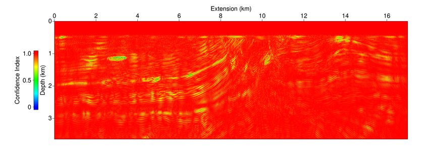
1. Introduction

   An application of seismic imaging is delineating the structural geologic aspects of the subsurface.
A migrated image is inferred from seismic data after careful processing and migration that intends
to collapse diffraction and relocates seismic reflections events to their correct position in depth. The
generation of images for seismic interpretation needs a migration tool, which has as inputs seismograms
and an estimation of the spatial velocity distribution. This data is acquired from seismic measurements
with appropriated pre-processing and velocity analysis techniques, like Normal Move-Out, tomography,
or full-waveform inversion (FWI).
   In seismic exploration, many decisions rely on interpretations of seismic images, which are affected by
multiple sources of uncertainty. The leading causes of uncertainty in seismic imaging are the geometry
survey, source signature, data noise, data processing, parameters, and model and numerical errors [1, 2].
Such procedures lead, unavoidably, to uncertainties on the data that propagate to the velocity analysis
and migration process. The effects of such uncertainties are hard to quantify. Thus, fundamental to the
decision-making process is understanding uncertainties and how they influence the outcomes. Building a
depth seismic migrated image is challenging due to the non-uniqueness of the inverse problem to estimate
the uncertain velocity parameters.
   Several works discuss how to express the uncertainty related to velocity-model building and measure
the impact on the migration techniques [1, 2, 3, 4, 5, 6]. Typically, uncertainties are characterized
through a probabilistic perspective and expressed as an ensemble of possible realizations of a random
variable, making the Monte Carlo (MC) method the standard tool to manage and quantify uncertainties
[7, 8, 9, 10, 11, 12]. Furthermore, these works emphasize the computational difficulties in quantifying
the uncertainties, particularly those associated with the high dimensionality of the data. For instance,
[3] and Poliannikov and Malcolm [4] choose smart sampling strategies to overcome the computational
limits of calculating posteriors for more realistic problems. We recall that to access uncertainties is
necessary to migrate the recorded data in several hundreds of samples. Migrating the samples makes
the computational algorithms not only time but also data intensive. Even in today’s supercomputers,
their implementation and data management become critical for the effective implementation of seismic
imaging with quantified uncertainty.
   To tackle the computational and data management challenges on seismic imaging with quantified
uncertainty, we introduce a workflow built upon three sequential stages: (i) Bayesian tomography to
estimate the seismic velocity from first arrival travel times, where the forward modeling relies on the
Eikonal equation (called here Bayesian Eikonal Tomography - BET), and the Reversible Jump Monte
Carlo Markov Chain (RJMCMC) algorithm [13, 14, 9]; (ii) Seismic migration using Reverse Time Mi-
gration (RTM) wrapped in a Monte Carlo algorithm; (iii) Image interpretation supported by statistical
information. The BET inversion for velocity estimation offers the flexibility of treating any prior informa-
tion, like a reasonable initial velocity estimation, and it has the advantage of providing results that help

                                                     2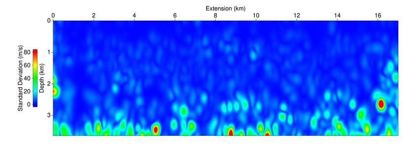
to quantify the uncertainties associated with the solutions [9]. RTM migrates the seismograms for the
velocity models from the first stage (BET) to generate the corresponding set of migrated seismic images.
Lastly, we expose the uncertainty maps that give a global representation of the ensemble of velocity fields,
and images produced respectively by BET and RTM.
   Model-selection strategies [3] can decrease the number of models for the migration stage. Neverthe-
less, even in this case, RTM migration wrapped into the Monte Carlo method is still challenging due
to the high dimensional uncertain inputs, the amount of data to manage, and computational costs as-
sociated with imposing the Courant-Friedrichs-Lewy (CFL) condition for the two-way wave equation.
Therefore, we present a parallel solution for RTM with quantified uncertainty to mitigate the compu-
tational costs. Our implementation explores MPI to manage each RTM among distributed platforms,
and OpenMP+vectorization to explore parallelism in hybrid architectures. Besides, data compression
[15] improves data transfer through the workflow stages, to read the seismogram from disk, to manage
temporary files, and to store the results in the final stage. Data compression is necessary because the
workflow generates a large amount of heterogeneous data. Finally, to manage and track data exchange
among the stages, we capture provenance data to monitor the several file transformations in addition to
registering CPU, file paths, and relationships among files.
   This work is organized by initially briefly reviewing the essential components to build the workflow.
After that, we detail the workflow with an emphasis on providing uncertainty estimations on the results.
We discuss in the sequence high-performance computing improvements for RTM, and the additional data
management tools for data compression and provenance. The paper ends with a summary of our main
conclusions.

2. Bayesian Eikonal Tomography

   In this section, we present the main concepts supporting our probabilistic framework for seismic
imaging with quantified uncertainty. Bayesian inference states the solution of an inverse problem as a
posteriori probability distribution (pdf) [16] of a random variable (often random fields), which in our case
is a function that describes the spatial distribution of the heterogeneous subsurface velocity given the
observed data. However, the posterior distribution cannot be expressed in a convenient analytical form
[7]. Hence, to address this problem, we use a Markov Chain Monte Carlo (MCMC) method to generate
samples of the stochastic field. The samples ensemble serves as input data for generating seismic images,
producing a migration with quantified uncertainty.

2.1. Migration with Quantified Uncertainty
   Seismic tomography is an inversion tool that aims to identify physical parameters (velocity, anisotropy,
among others) given a set of observations (measurement data). Parameters and the data are related by
the following equation:

                                          dobs = F(m) + ,                                              (1)

                                                     3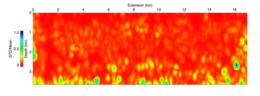
where is an additive noise including modeling and measurements errors. Here, the operator F is the
Eikonal equation, that connects the velocity with first arrival travel times [17]. The high-dimensional
parameter vector m = (V, U, n), where n is the number of grid points, the n-dimensional vector U = {ui },
contains the grid positions, and the vector V = {vi }, i = 1, 2, . . . n, the velocity of the compressional
wave in the i-th computational grid point.
Iterative linearized approaches for seismic tomography have problems related to non-linearity and ill
- posedness. These methodologies usually produce inaccurate parameters due to local minimum conver-
gence. Besides, iterative linearized methods are not able to properly quantify the uncertainty associated
with their solution. To address this issue, we have chosen a Bayesian formulation to aggregate as infor-
mation as possible to yield a better parameter estimation and the associated uncertainties. A Bayesian
approach aims at estimating the parameters conditional distribution with respect to known data, through
a combination of prior knowledge regarding the velocity model and information provided by such data.
Thus, to define the posterior distribution P (m|dobs ), we use Bayes’ theorem:
P (dobs |m)P (m)
P (m|dobs ) = , (2)
P (dobs )
where P (dobs |m) is the likelihood function, P (m) is the a priori parameter density distribution, and
P (dobs ) is the evidence.
The likelihood represents how well the estimated travel times fits the measurements. Assuming that
the additive noise in Equation 1 is Gaussian with zero mean and variance σd2 the likelihood is:
2
obs
1 F (m) − d
P (dobs |m) = exp − , (3)
2 σd2
where k · k is the standard l2 -norm.
To explore the posterior distribution and deal with the space parameter dimension, we employ the
Reversible Jump Markov Chain Monte Carlo (RJMCMC) method [13, 14, 7, 9]. The MCMC method is
an iterative stochastic approach to generate samples according to the posterior probability distribution.
A generalized version, called Reversible Jump, allows inference on both parameters and its dimensionality
[7]. Thus, following [9], we employ a Voronoi’s tesselation with Gaussian kernels as basis functions to
constrain the inverse problem solution and reduce the parameter dimensionality. Such parametrization
works as a prior that embodies the expected velocity field non-stationary character, displaying localized
abrupt changes with a continuous variation. Hence, the number of Voronoi cells n0
n. Therefore, given
the current state of the chain mi , three perturbations are possible, that is, the probability of adding (pa )
new cell nuclei, probability of deleting (pd ) one existing cell nuclei, and the probability of moving (pm )
selected cell nuclei. Hence, the acceptance probability of the three perturbations depends on the ratio
of their likelihoods. After a burn-in phase, the process iterates, eventually reaching the total number
of pre-defined iterations. By attributing a constant velocity magnitude inside each Voronoi cell, we put
a probabilistic structure in the prior, assuming that such velocity values follow independent uniform
4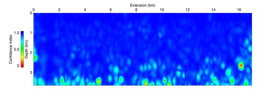
variables. Playing with the bound of the random variables, we can incorporate in the priors spatial
trends learned by experts by different data sources, like the deposition history.

2.2. Reverse Time Migration
   Reverse Time Migration (RTM) is a depth migration approach based on the two-way wave equation
and an appropriate imaging condition. Restricting ourselves to the acoustic isotropic case, the wave
equation is,
                                                          1    ∂ 2 p(r, t)
                                     ∇2 p(r, t) −                          = 0,                                (4)
                                                     v 2 (r)       ∂t2
where r = (rx , ry , rz ) is the position vector, v is the compressional wave velocity, and p(r, t) the hydrostatic
pressure in the position r and time t.
   The RTM imaging condition [18] is the zero-lag cross-correlation of the forward-propagated source
wavefield (S) and the backward-propagated receiver wavefield (R) normalized by the square of the source
wavefield,
                                                 R
                                                     T
                                                         S(r, t)R(r, t)dt
                                        I(r) =           R                .                                    (5)
                                                          T
                                                            S 2 (r, t)dt
   The source wavefield is the solution of equation 4 with the seismic wavelet treated as a boundary
condition. Similarly, the receiver wavefield is the solution of the same equation 4 with the observed
data (seismograms) as a boundary condition. The normalization term in equation 4 produces a source-
normalized cross-correlation image that has the same unit, scaling, and sign as the reflection coefficient
[18]. Therefore, within the MC method, RTM migrates the near-surface recorded signals for the ensemble
of BET-generated velocity samples.

2.3. Uncertainty in Images
   To reach a global representation of the solution variability within the ensemble of plausible velocity
fields and images produced by the workflow, we follow [19]. They proposed a confidence index, that
normalizes the uncertainty map explored by Li et al. [3], that assigns at each spatial point an evaluation
of the degree of uncertainty expressed by the standard deviation σ(r), where low values represent regions
where there are high variabilities, and high values the regions where there are small variabilities. The
confidence index is expressed by,
                                                         σmax − σ(r)
                                           c(r) =                    ,                                         (6)
                                                         σmax − σmin
where c(r) is the confidence in position r, and σmin , σmax and are the minimum, maximum and standard
deviations in the r position, respectively.
   An alternative measure is the ratio between standard deviation and average, that is,
                                                              σ(r)
                                                 r(r) =            ,                                           (7)
                                                              µ(r)
where, µ represents the average map of the data. In this case, Equation 7 measures the variations among
the samples with the mean as reference.

                                                               5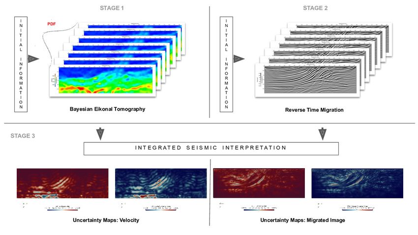
3. A Workflow for Seismic Imaging

    In this section, we present the components of our workflow for seismic imaging with quantified uncer-
tainty. We have chosen a particular set of chained components that provide a comprehensive probabilistic
framework for seismic imaging. Nevertheless, we recognize that different components could be chained
in a similar form to provide other possible workflows. Thus, a workflow is an abstraction that represents
stages of computations as a set of activities and a data flow among them. Each activity can be a software
that performs operations on an input data set, transforming it into an output data set. A workflow can
represent the whole seismic imaging stages as a chain of activities. Stages of seismic imaging (or workflow
activities) can be replaced or extended to build a different viewpoint of the outcomes, such as statistic
information for uncertainty quantification.
    Figure 1 shows the three workflow stages. BET produces an ensemble of velocity fields (stage 1),
RTM generates the corresponding seismic images (stage 2), and stage 3 builds the uncertainty maps
for the velocity and migrated images from the results of stages 1 and 2. To efficiently implement this
workflow, we address three computational aspects: parallelism, data transfer, and data management.
Figure 2 describes how the workflow produces the ensemble of velocities and migrated images for posterior
uncertainty quantification, the hybrid parallelism in the RTM stage, and where data compression is used
to reduce storage and network data transfer.

Figure 1: Results of BET (Stage 1), and RTM for each velocity field (Stage 2) built-in Stage 1. Stage 3 shows the uncertainty
maps for velocities and migrated images. The maps can guide interpreters to potential areas with low/high uncertainty in
velocities and structures.

    Stage 1 aims to build a probabilistic density function for the velocity encompassing feasible solutions

                                                             6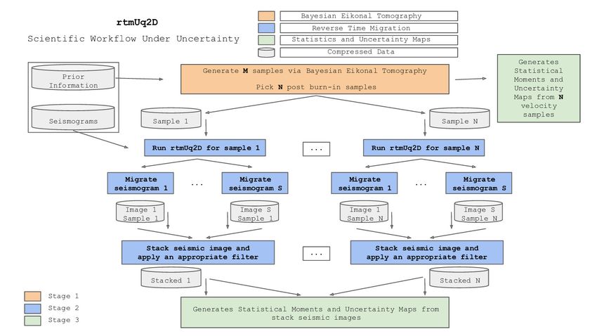
that fit the calculated travel times to the data and provides enough information for the next two stages.
To generate samples of the stochastic field, BET needs to run thousands of RJMCMC iterations. In the
Voronoi’s tessellation within RJMCMC the number of cells, their position and size vary. This strategy
produces a number of Voronoi cells smaller than the velocity parameters, as a cell might contain many
computational grid points. We use a KD-tree [20] to reduce the searching cost in the Voronoi’s tessellation
updating. Solving the Eikonal wave equation in each iteration dominates BET costs. We use here the
open-source software FaATSO8 to solve the Eikonal wave equation.

Figure 2: Stage 1 provides a probabilistic distribution of velocity using BET. Stage 2 migrates the seismograms for all
velocity parameters, generating, thus, a set of stacked seismic sections. Finally, Stage 3 extracts statistical information from
velocity parameters and migrated images. Compression is used to transfer the data among the stages. Step 2 uses rtmUq2D
a hybrid parallel RTM code.

    At the end of stage 1, we select a set of velocities for the migration based on the variance of successive
batches of the post-burn-in samples. Thus, when the stochastic process converges, the variance among
the samples stabilizes. In the second stage, RTM migrates the seismograms for the sub-set of velocity
fields. These migrations produce the corresponding set of seismic images, where each one has a direct
relation with one velocity sample coming from stage 1. To attenuate low-frequency artifacts in the brute
stack images, we apply a Laplacian filter. The RTM kernel, that is, the second-order wave equation,
is discretized with a second-order finite difference scheme in time and an eighth-order scheme in space.
The reverse problem implementation explores the technique proposed by [21]. This technique guarantees
the coercivity of the adjoint problem. Furthermore, the RTM code, rtmUq2D, takes advantage of the

   8 Fast   Marching Acoustic Emission Tomography using Standard Optimization: https://github.com/nbrantut/FaATSO

                                                               7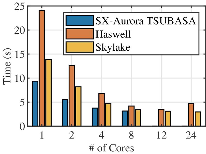
Single-Instruction-Multiple-Data (SIMD) model and memory alignment allocation to ensure vectoriza-
tion. rtmUq2D also contains OpenMP directives to explore multiple cores parallelism. To complete our
hybrid RTM solution, we apply MPI to manage the execution of multiple migrations and shots. Thus, we
broke the total number of migrations into subgroups, and each subgroup is assigned to an MPI process,
as exemplified in Figure 2. When a subgroup finishes its workload, the next one starts immediately.
The batch execution (an RTM for each subgroup) is repeated until exhausting the number of samples.
Besides, each RTM verifies its own CFL condition to guarantee the stability of the discrete solution of
the two-way wave equation for each sample.
   Once stages 1 and 2 produce ensembles of velocity fields and seismic images, a condensed repre-
sentation of this information can be calculated. In stage 3, velocity uncertainty maps are obtained as
soon as we accept BET solutions. The same procedure is valid for generating migrated images. Hence,
stage 3 generates uncertainty maps representing variability in velocity, and reflectors amplitudes. These
outcomes give to geoscientists extra information to guide the seismic interpretation.
   However, to better support interpretation and improve confidence, it is essential to register relation-
ships between data produced at each workflow stage. For example, the uncertainty maps of stage 3 are
related to the velocity fields and statistics, which are also related to the seismic images. Tracking these
data derivations among the stages at runtime, combined with the procedures’ execution time, can sup-
port workflow parameters debugging and fine-tuning. Provenance data [22] represents the data derivation
path of the data transformations during the stages. Provenance data capture and storing in a prove-
nance database while the workflow executes can add an overhead to the workflow execution. We choose
DfAnalyzer as a provenance asynchronous data capture software library because it can be used by high
performance computing (HPC) workflows to provide for runtime data analysis with negligible overhead
[23]. While monitoring the workflow execution, users submit queries to the travel time matrix during
the migration or go directly from an input velocity model file to the corresponding files that have their
statistics obtained after all samples were aggregated. DfAnalyzer has been successfully used for other
HPC applications [24, 25].
   Data transfer is also a concern when each stage in the workflow has to manage its information and
send it to the next workflow stage. The amount of data transfer can increase drastically, given the
number and size of the samples in the ensemble of velocities and migrated images. Data compression
can reduce persistent storage and data transfer throughout the chain [15]. The ZFP library is an open-
source C/C++ library for compressing numerical arrays. To achieve high compression rates, ZFP uses
lossy but optionally error-bounded compression. Although bit-for-bit lossless compression of floating-
point data is not always possible, ZFP also offers an accurate near-lossless compression [15]. We employ
ZFP to compress the numerical arrays that store the velocity parameters, imaging conditions, and the
seismograms. This use is linked to the workflow stages to reduce the pressure on the network data transfer
among the workflow stages and to reduce I/O to persistent storage. However, lossy compression has to
be managed carefully, and with safe error-bounds. We test both lossy and lossless compression, and we

                                                    8
measure the error on the final results.
4. Computational Experiments
We designed some computational experiments to assess the overall workflow behavior and perfor-
mance. They consist of verifying RTM strong and weak scalability, measuring the numerical errors on
the final results after applying data compression, and discussing the workflow uncertainty quantification
outcomes using the data analysis tools. We choose two datasets: a two-layer constant velocity field for
scalability analysis, and one based on the 2-D Marmousi2 benchmark [26] for applying data compression
and running the full workflow.
4.1. Scalability Analysis
We choose a two-layer constant velocity model that is 3.0 km depth and 9.2 km in the horizontal
direction for the scalability tests. The velocities for the two layers are 2000 m/s, and 3000 m/s. We
generate the reference data set for RTM based on the true velocity field. The reference data set is the
wavefield recorded by near-surface hydrophones (one seismogram) with a cutoff frequency of 30 Hz. The
input velocity field for RTM is a smooth version of the synthetic velocity model.
Figure 3 shows the RTM strong scalability considering a migration of one shot for an increasing number
of cores. We run the tests on different platforms: 1 vector processor (NEC SX-Aurora TSUBASA TypeB),
and 2 multi-cores CPUs (Intel Xeon E5-2670v3 (Haswell) and Intel Xeon Platinum 8160 (Skylake) CPUs).
The vector processor available has its minimum configuration, that is, 8 cores, while Haswell and Skylake
have 24 cores each.
Figure 3: RTM scalability analysis on different platforms. The tests consist of a migration for one seismogram. The vector
processor available has 8 cores, while Haswell and Skylake have 24 cores each.
9The code is portable across the different platforms requiring only the necessary compiler options for
each system to enable aggressive optimization. Compiler flags are invoked for NEC vector instructions
in SX-Aurora TSUBASA, Intel AVX2 vector instructions in Haswell, and Intel AVX512 instructions in
Skylake. In all systems, the wave-equation kernels are 100% vectorized. We can see that RTM on the
vector processor runs faster than in Haswell and Skylake platforms, without a specific optimization effort
for SX-Aurora TSUBASA.
Now we investigate the weak scalability. Due to our need to run the RTM n times to build the
statistics outcomes, the hybrid RTM has to run n times in n nodes. In this case, the CPU time for each
node has to be approximately the same. Assuming the same parametrization of the strong scalability
test, we run the RTM code for an increasing number of nodes and measure the CPU time for each one.
We note that the RTM takes, on average, 3.281s with standard deviation 0.0578s to execute one RTM
per node on the Haswell cluster. Thus, the CPU time for running one RTM in one node is approximately
the same as running five RTM in five nodes. We observe the same pattern for the other platforms.
4.2. Data Compression
We select the 2-D Marmousi2 velocity model benchmark [26] for the data compression experiments.
The benchmark is 3.5 km depth and 17.0 km in the horizontal direction and has parameters models
(p-wave velocity and density), and other data sets related to its acquisition. However, we generate the
seismograms solving the two-way wave equation with true velocity. Near-surface hydrophones record the
seismogram with a cutoff frequency of 45 Hz. Thus, we have 160 seismograms to be used in the migration
stage. In the BET stage, the reference data set is 34 travel-time panels obtained from solving the Eikonal
equation with true velocity.
After BET, we pick 5000 post-burn-in velocity models for migration. Thus, the RTM produced 5000
seismic images that corresponding with each velocity model from stage 1. Hence, we use 5000 velocity
models, 5000 seismic migrations, and 160 seismograms to test the lossy and lossless rate compression.
Table 1 shows the results related to compression efficiency for the velocity models and seismic images.
The compression efficiency for the seismograms are in Table 2.
Table 1: Fixed accuracy lossy and lossless compression comparison. The error tolerances for lossy compression are 10−4 ,
and 10−1 . Each value is the average of the 1000 compressed matrices (velocity fields, and seismic images).
Compression Velocity (MB) Image (MB)
None 6.10 6.10
Lossless 4.78 5.34
Lossy (10−4 ) 4.77 3.65
−1
Lossy (10 ) 2.98 1.83
Each velocity model and the seismic image without compression has 6.1 MB. The values in the columns
”Velocity” and ”Image” represent, respectively, the average size of 1000 matrices for the velocity models
10and seismic images without compression (first line), and with lossless and lossy compression. We apply
three compression types: the first one is lossless compression, the second one is lossy compression with an
absolute error of 10−4 , and the last one is lossy compression with an absolute error of 10−1 . We can see
that the lossy compression achieves the best compression rate, reaching about 51.1% of compression for
the velocity models (2.98 MB), and about 70.0% of compression for the seismic images (1.83 MB). Note
that the compression rates for each matrix are different since ZFP explores the structure of the data.
Although less efficient, the lossless compression reaches about 21.6% of compression for the velocity
models (4.78 MB) and about 12.5% of compression for the seismic images (5.34 MB). This efficiency rate
for lossless compression is compatible with its purpose, which is to preserve the original information.
We also apply lossless and lossy compression to the 160 seismograms. Each seismogram has 76.20
MB. The error tolerance for lossy compression is to 10−4 . Compression rates reach a minimum of 13.38
MB and a maximum of 8.38 MB, as we can see in Table 2. These values represent 82.4%, and 89.0% less
than the original data, respectively.
Table 2: Seismograms fixed accuracy lossy and lossless compression comparison. The error tolerance for lossy compression
is set to 10−4 . The values represent the minimum and maximum compression among the 160 seismograms.
Compression Type Minimum (MB) Maximum (MB)
None 76.20 76.20
Lossless 59.28 48.46
Lossy 13.38 8.38
The results from Table 1, and Table 2 suggest that we can use compressed data on the workflow and,
thus, reduce the storage and network data transfer. However, we need to measure the error propagation
due to compression on the final seismic images. Therefore, to measure the compression errors, we run RTM
to migrate the seismograms without compression with an uncompressed velocity model as a parameter.
Figure 4(a) shows the migration of the uncompressed seismograms, and Figure 4(d) shows the 2D Fourier
spectra of the two white boxes shown in Figure 4(a). The described outcomes are the reference once
we do not use ZFP compression. The same procedure is applied using the lossless compression of the
velocity model and seismograms as entries for RTM migration, and the lossy compression (tolerance error
of 10−4 ) of the velocity model and seismograms as entries for RTM migration. These results can be seen
in Figures 4(a)(e), and Figures 4(c)(f), respectively.
We calculate the normalized root mean square (NRMS) error among the RTM results from Figure 4(a),
and the RTM results from Figures 4(b), and 4(c). The NRMS errors are 2.0 × 10⁻⁶ % and 4.3 × 10⁻⁵ %,
respectively. The NRMS errors among the spectra from the left white box regions in Figures 4(a), 4(b)
and 4(c) are 1.1 × 10⁻⁶ %, and 1.97 × 10⁻⁵ %, respectively. Moreover, the NRMS errors among the spectra
from the right white box regions in Figures 4(a), 4(b) and 4(c) are 1.3 × 10⁻⁶ %, and 2.6 × 10⁻⁵ %,
respectively. The results from Figure 4 and the NRMS errors show that the chosen compression levels
11for the velocity models and seismograms lead to migrated images with errors of order 10−5 %. The
compression strategy allows to reduce 85% in storage, and, consequently, improves network data transfer
without compromising accuracy.
Figure 4: RTM outcomes after migrating the (a) reference seismograms, seismograms with (b) lossless compression, and
seismograms with (c) lossy compression. The velocity field inputs are not compressed for migration in Figure (a), losslessly
compressed for migration in Figure (b), and lossy compressed for Figure (c). Figures (d), (e), and (f) represent the 2D
Fourier spectra of the white box regions shown in Figures (a), (b), and (c), respectively.
4.3. Provenance Data Queries
Provenance data is captured to analyze data from the several workflow stages by DfAnalyzer and
stored in a columnar database using the MonetDB system9 . The workflow needs to have a definition
of which data should be part of the provenance database. Then, DfAnalyzer calls are inserted in the
workflow code to capture data provenance, as shown in Listing 1. We run a series of RTMs with and
without DfAnalyzer calls. In all tests, the overhead of provenance data capture and storage remains
below 2.95%, as shown in Table 3. Also, the overhead rate decreases as the number of nodes increases.
During and after the workflow executions, queries can be submitted to the provenance database using
filters or data aggregations over the workflow stages data derivation path, as shown in Figure 5.
4.4. Seismic Imaging Uncertainty Quantification
We discuss here the results of sequentially applying BET and RTM to the raw data provided by
seismograms generating images with quantified uncertainty. The ensemble of uncertain velocity fields
9 https://www.monetdb.org
12Table 3: RTM overhead with DfAnalyzer calls. Each node executes two RTMs.
# of Nodes # of RTMs Overhead (%)
1 2 2.95
2 4 2.63
4 8 1.26
5 10 1.02
shot shot
shot Location Location seismogram path cross correlation path
(x) m (z) m
1 25.00 25 ./.../seisNorm 001.bin ./.../crossCorre 001X001.bin
2 131.25 25 ./.../seisNorm 002.bin ./.../crossCorre 002X001.bin
3 237.50 25 ./.../seisNorm 003.bin ./.../crossCorre 003X001.bin
4 243.75 25 ./.../seisNorm 004.bin ./.../crossCorre 004X001.bin
5 450.00 25 ./.../seisNorm 005.bin ./.../crossCorre 005X001.bin
6 556.25 25 ./.../seisNorm 006.bin ./.../crossCorre 006X001.bin
7 662.50 25 ./.../seisNorm 007.bin ./.../crossCorre 007X001.bin
8 768.75 25 ./.../seisNorm 008.bin ./.../crossCorre 008X001.bin
9 875.00 25 ./.../seisNorm 009.bin ./.../crossCorre 009X001.bin
10 981.25 25 ./.../seisNorm 010.bin ./.../crossCorre 010X001.bin
Figure 5: Provenance query result showing the shots with their (x, z) location and the path of their corresponding seismogram
image file and the cross correlation file, filtered by a shot location where z = 25 and 0 < x < 1000.
resulting from BET is assessed through primary statistics, such as velocity mean and standard deviation.
In the sequence, we compute uncertainty maps. After the RTM migrates the seismograms for each
velocity field, we analyze the impact of the inversion uncertainties in the seismic images. Note that in
this stage, we choose to work on the compressed seismograms and velocity fields to reduce the storage and
network transfer. As we show in Figure 4, the lossy compression for both velocity and seismograms, with
an error tolerance of 10−4 , does not produce migrated seismic images with poor quality. Hence, we use
them in the whole workflow. Besides, the Marmousi2 benchmark, as specified in Sub-section 4.2, is used
to demonstrate the outcomes of the workflow. To keep track of the impact of each uncertainty source, we
restrict the analysis in this particular example to the noise associated with monitoring the data, defined
by σd2 in equation 1. The other component that would induce uncertainty would be the scarcity of data
promoted by acquiring signals only on the surface. That is circumvented by collecting the synthetic data
13in all grid points. We anticipate facing a lower degree of uncertainty in the final images due to such a
choice.
1 int task_id = 1;
2 Task task_runrtm = Task ( dataflow . get_tag () , runrtm . get_tag () , task_id ) ;
3
4 vector < string > irun rtm_val ues = { velocityFile , waveletFile , std :: to_string ( Nx ) , std :: tostring ( Nz ) };
5 Dataset & ds_irunrtm = task_runrtm . add_dataset ( irunrtm . get_tag () ) ;
6 ds_irunrtm . a d d _ e l e m e n t _ w i t h _ v a l u e s ( ir unrtm_va lues ) ;
7
8 // rtm per shot
9 for ( shotID = 1; shotID i s e i s m o g r a m _ v a l u e s = { s e i s m o g r a m F i l e _ 0 2 };
20 Dataset & ds_iseis mogram = task_runrtm . add_dataset ( iseismogram . get_tag () ) ;
21 ds_iseismogr am . a d d _ e l e m e n t _ w i t h _ v a l u e s ( i s e i s m o g r a m _ v a l u e s ) ;
22
23 task_runrtm . begin () ;
24 // end input registration
25
26 reading_file ( seismogramFile_02 , seismogram , numberOfReceivers , n u m be r O f T i m e S t e p ) ;
27
28 // backward modeling
29 adjoint M od el in g ( shotID , shotLocation , velocityModel , wavelet , seismogram ) ;
30
31 // begin DfAnalyzer output registration
32 if ( shotID == numberOfShots )
33 task_runrtm . end () ;
34 else task_runrtm . save () ;
35 // end output registration
36 }
Listing 1: This workflow code shows DfAnalyzer calls inserted before RTM stage runrtm.begin to capture and register the
input: velocityFile; wavelet and seismogram path with the corresponding output: cross-correlation file path after the RTM
execution runrtm.end explicitly relating input and output data in the provenance database.
Figure 6 shows the standard deviation (top), confidence index (middle), and standard deviation over
the mean value (bottom) of the velocity fields. The standard deviation field expresses the degree of
uncertainty in the velocity at each point of the domain. The minimum standard deviation values are
around 1 m/s and localized in shallow regions. On the other hand, the maximum standard deviation
values occur in deeper regions with values around 80 m/s. The confidence index (Equation 6) is the
normalized standard deviation and represents the confidence degree in the velocities [3]. We depict in
Figure 6 (middle) the confidence index within the image domain. We can see that such criterion assigns
14higher confidence (> 0.8) to shallow regions. Figure 6 (bottom) shows r(r) map. Again we observe the
same trends.
Figure 6: Figures show the standard deviation (top), confidence index (middle) and r(r) map (bottom) of the Marmousi
velocity fields.
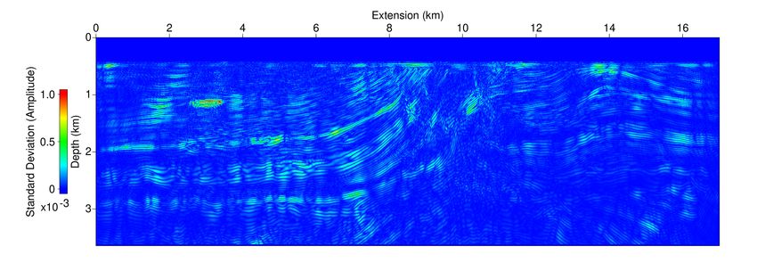
We plot in Figure 7 (top) the standard deviation for a representative image computed as an average
amongst those of the ensemble. Besides, we plot the confidence index (middle) and r(r) map (bottom)
of the seismic images obtained from RTM wrapped on the MCMC. In this case, the observed variations
are related to the amplitude of the reflections instead of p-wave velocity. That is the variability of
the amplitude intensity. This one is maximum in the interface between two rocks with different physical
properties. However, if an estimated p-wave velocity differs from the exact p-wave velocity of the medium,
the amplitude intensity is misplaced. Hence, the high standard deviation, low confidence index, and low
standard deviation over the mean values are highlighted in the interfaces and predominant in the middle
region.
15Figure 7: Figures show the standard deviation (top), confidence index (middle) and r(r) map (bottom) of the migrated
seismic images. RTM migrates 160 seismograms for each velocity field.
5. Conclusions
We proposed a new scientific workflow that supports uncertainty quantification in seismic imaging.
Our stochastic perspective to handle uncertainties is composed of three sequential stages: inversion,
migration, and interpretation. A Bayesian tomography (Stage 1) provides the input data for the RTM
wrapped on the MCMC (Stage 2). The workflow deploys means to end-users to explore uncertainty in
the final images through maps computed in Stage 3.
The workflow execution requires significant computing power and generates a huge amount of data.
Thus, we use optimized hybrid computing solutions that explore vectorization, data compression, and
advanced data management tools. These tools allow us to obtain a scalable solution for the Marmousi
Velocity Model benchmark with quantified uncertainty. ZFP compression has been used to transfer
information among the stages and to store the final images. High levels of compression have been
observed for the ensembles of velocities and migrated images. The compression strategy improves the
network data transfer and reduces the amount of data up to 85%, assuming a tolerance error of 10−4
without affecting the quality of the final result. The provenance database keeps a record of the workflow
16execution stages enriching the seismic data analysis quality. We observed that capturing and storing
provenance data during the workflow execution is inexpensive.
Acknowledgements
This study was financed in part by CAPES, Brasil Finance Code 001. This work is also partially
supported by FAPERJ, CNPq, and Petrobras. Computer time on Stampede is provided by TACC, the
University of Texas at Austin. The US NSF supports Stampede under award ACI-1134872. Computer
time on Lobo Carneiro machine at COPPE/UFRJ is also acknowledged. We are also indebted to NEC
Corporation.
Computer Code Availability
The codes can be downloaded at the repository https://github.com/Uncertainty-Quantification-Project.
The repository provides three opensource codes (bayes-tomo, rtmUq2D, and rtmUq2D-Prov). The user
guide describes the software and hardware requirements, and directs to complementary opensource soft-
ware used in the paper.
References
[1] J. Caers, Modeling uncertainty in the earth sciences, John Wiley & Sons, 2011.
[2] S. Fomel, E. Landa, Structural uncertainty of time-migrated seismic images, Journal of Applied
Geophysics 101 (2014) 27–30.
[3] L. Li, J. Caers, P. Sava, Assessing seismic uncertainty via geostatistical velocity-model perturbation
and image registration: An application to subsalt imaging, The Leading Edge 34 (2015) 1064–1070.
[4] O. Poliannikov, A. Malcolm, The effect of velocity uncertainty on migrated reflector: Improvements
from relative-depth imaging, Geophysics 81 (2016) S21–S29.
[5] J. Messud, M. Reinier, H. Prigent, P. Guillauma, T. Coléou, S. Masclet, Extracting seismic uncer-
tainty from tomography velocity inversion and their use in reservoir risk analysis, The Leading Edge
36 (2017) 127–132.
[6] G. Ely, A. Malcolm, O. Poliannikov, Assessing uncertainty in velocity models and images with a
fast nonlinear uncertainty quantification method, Geophysics 83 (2018) R63–R75.
[7] T. Bodin, M. Sambridge, Seismic tomography with reversible jump algorithm, Geophysical Journal
International 178 (2009) 1411–1436.
[8] A. Botero, A. Gesret, T. Romary, M. Noble, C. Maisons, Stochastic seismic tomography by inter-
acting markov chains, Geophysical Journal International 207 (2016) 374–392.
17[9] J. Belhadj, T. Romary, A. Gesret, M. Noble, , B. Figliuzzi, New parametrizations for bayesian
seismic tomography, Inverse Problems 34 (2018) 33.
[10] D. G. Michelioudakis, R. W. Hobbs, C. C. S. Caiado, Uncertainty analysis of depth predictions
from seismic reflection data using bayesian statistics, Geophysical Journal International 213 (2018)
2161–2176.
[11] J. Martin, L. C. Wilcox, C. Burstedde, O. Ghattas, A stochastic newton mcmc method for large-
scale statistical inverse problems with application to seismic inversion, SIAM Journal on Scientific
Computing 34 (2012) A1460–A1487.
[12] N. Rawlinson, A. Fichtner, M. Sambridge, M. K. Young, Chapter one - seismic tomogra-
phy and the assessment of uncertainty, volume 55 of Advances in Geophysics, Elsevier, 2014,
pp. 1 – 76. URL: http://www.sciencedirect.com/science/article/pii/S0065268714000028.
doi:https://doi.org/10.1016/bs.agph.2014.08.001.
[13] P. J. Green, Reversible jump markov chain monte carlo computation and bayesian model determi-
nation, Biometrika 82 (1995) 711–732.
[14] P. J. Green, D. I. Hastie, Reversible jump mcmc, Genetics 155 (2009) 1391–1403.
[15] P. Lindstrom, P. Chen, , E.-J. Lee, Reducing disk storage of full-3d seismic waveform tomography
(f3dt) through lossy online compression, Computers & Geosciences 93 (2016) 45–54.
[16] A. F. M. Smith, Bayesian computational methods, Philosophical Transactions: Physical Sciences
and Engineering 337 (1991) 369–386.
[17] N. Brantut, Time-resolved tomography using acoustic emissions in the laboratory, and application
to sandstone compaction, Geophysical Journal International 213 (2018) 2177–2192.
[18] H.-W. Zhou, H. Hu, Z. Zou, Y. Wo, O. Youn, Reverse time migration: A prospect of seismic imaging
methodology., Earth-Science Reviews 179 (2018) 207–227.
[19] Y. Li, J. Sun, 3d magnetization inversion using fuzzy c-means clustering with application to geology
differentiation, Geophysics 81 (2016) J61–J78.
[20] M. B. Kennel, KDTREE 2: Fortran 95 and C++ software to efficiently search for near neighbors in
a multi-dimensional Euclidean space (2004). arXiv:0408067.
[21] D. Givoli, Time reversal as a computational tool in acoustics and elastodynamics, Journal of
Computational Acoustics 22 (2014) 45–54.
[22] S. B. Davidson, J. Freire, Provenance and scientific workflows: challenges and opportunities, in: in
Proceedings of the 2008 ACM SIGMOD International Conference on Management of Data, 2008,
pp. 1345–1350.
18[23] V. Silva, D. de Oliveira, P. Valduriez, M. Mattoso, Dfanalyzer: runtime dataflow analysis of scientific
applications using provenance, Proceedings of the VLDB Endowment 11 (2018) 2082–2085.
[24] J. J. Camata, V. Silva, P. Valduriez, M. Mattoso, A. L. G. A. Coutinho, In situ visualization and
data analysis for turbidity currents simulation, Computers & Geosciences 110 (2018) 23–31.
[25] V. Silva, J. Camata, D. De Oliveira, A. Coutinho, P. Valduriez, M. Mattoso, In situ data steering on
sedimentation simulation with provenance data, in: SC: High Performance Computing, Networking,
Storage and Analysis, 2016.
[26] R. Wiley, M. K. J., Marmousi2: An elastic upgrade for marmousi, The Leading Edge 25 (2006)
156–166.
19You can also read