Google Earth Engine Tools for Long-Term Spatiotemporal Monitoring of Chlorophyll-a Concentrations

Open Water Journal – Volume 7, Issue 1, Article 4

Google Earth Engine Tools for Long-Term
Spatiotemporal Monitoring of Chlorophyll-a
Concentrations
Research Article
Anna Cardall1, Kaylee Tanner2, Gustavious Williams3
1
 Undergraduate student, Chemical Engineering, Brigham Young University, Provo, Utah 84602,
anna.cardall@gmail.com
2
 Graduate student, Civil and Environmental Engineering, Brigham Young University, Provo, Utah 84602
3
 Associate Professor, Civil and Environmental Engineering, Brigham Young University, Provo, Utah 84602

Abstract
 We present a set of Google Earth Engine (GEE) tools to process long-term satellite imagery to analyze the
time history of algal concentrations in a lake or reservoir. We demonstrate these tools with a case study on Utah
Lake, Utah, USA. Our tools collect and process Landsat surface reflectance images from three different Landsat
missions: Landsat 5, Landsat 7, and Landsat 8. These satellites represent data from 1984 until the present at 16-
day intervals: over 1,000 images, though not all images are usable due to weather, ice, and other issues. We
present the GEE commands or tools to mask these images to only include pixels in a selected region around a
selected water body (spatial masking); pixels that represent the water, as most water bodies change size due to
fluctuating water levels (classification masking); and pixels that meet a quality threshold to exclude pixels with
issues that affect model accuracy (quality masking). The quality masking excludes pixels that contain clouds,
significant atmospheric moisture, or other issues that would affect the accuracy of the data. We perform quality
masking based on metadata included in the Landsat level 2 data quality band. After masking, the remaining pixels
represent the extent of the visible water body at the time of the image. We use GEE to implement an empirical
model from the literature to estimate the chlorophyll-a (chl-a) concentration in each pixel for each image over the
entire 40-year history. The model is slightly different for different satellite collections. To determine if there are
trends in the data, we implemented the nonparametric Mann-Kendall test and applied it to the computed chl-a
concentration images. The Mann-Kendall test determines the presence, magnitude, and statistical significance of
algal growth trends. To demonstrate the Mann-Kendall test, we used a subset of 31 images from the month of
July over a 16-year period—1999 to 2015—and determined algal growth trends for each pixel during this period.
For our case study of Utah Lake, we found that there was no statistically significant trend in the majority of the
lake, with only the Provo Bay area, a hydrologically isolated bay, demonstrating a small statistically significant
upward trend. While the GEE tools we implemented have inputs specific to Utah Lake, Landsat data, and chl-a
concentrations, these tools can be easily modified and be applied to other lakes, satellites, and water quality

Open Water Journal – Volume 7, Issue 1, Article 4 2
parameters. If different satellites, lakes, or water quality parameters are used, then our empirical models and
spatial boundaries would need to be modified for the selected satellite, lake, and parameter.
Keywords: Earth Observation Data, Remote Sensing, Chlorophyll, Google Earth Engine, Automated Tools

1.0 Introduction
 Landsat data have been used extensively to assess algal blooms since the mid-1970s, with Utah Lake, the
location of our case study, being one of the first locations studied using these data (Strong, 1974). Since that time,
many other studies have followed (Klemas, 2012; Richardson, 1996; Stumpf, 2001). Earth observation data from
satellites allows us to easily examine spatial distributions of algae growth (Nelson et al., 2003; Olmanson et al.,
2008) by estimating chl-a concentrations, which indicate algal blooms (Brivio et al., 2001b; Ma & Dai, 2005;
Mayo et al., 1995; Wheeler et al., 2012). Some researchers have extended these studies to produce time-history
studies using Landsat images to study the time history of chl-a concentrations (Allan et al., 2015; Bonansea et al.,
2015; Ho et al., 2017; Yip et al., 2015), which yield a better understanding of spatial distributions and temporal
trends of algae growth in a lake or reservoir (Nelson et al., 2003; Olmanson et al., 2008).
 The Landsat satellites were specifically designed to monitor ecosystems by acquiring multispectral images
with spectral image bands selected to evaluate plant growth, water quality, and other parameters (Landsat—Earth
observation satellites, 2016). Data from the Landsat satellites are available starting in the 1970’s, with more useful
data starting with Landsat 5 in 1984. This makes Landsat data particularly valuable for evaluating long-term
trends and the health of ecosystems.
 Google Earth Engine (GEE) greatly simplifies the work required to download and process satellite images
(Hansen, 2015).(Hansen, 2015). Prior to the availability of GEE, a researcher would need to download and process
individual images, then use the resulting data to evaluate long-term trends. While software packages have
improved over the years, in most cases the user must still download individual images, calibrate each image before
analysis, and then process the resulting set of images to examine changes over time. Because of the amount of
work involved, our research group typically limited our data to a few images per year, and, based on our reading
of the literature, this approach seems typical. With GEE tools, the image acquisition, preparation, masking, and
empirical modeling can all be automated, allowing researchers to easily analyze more detailed long-term data.
GEE provides ready access to Level 2 data, which provide calibrated “surface reflectance” data or pre-calibrated
images. NASA defines “Level 2” data as “derived geophysical variables at the same resolution” as the source
data. For our studies, the derived value is the surface reflectance.
 To use Landsat data, researchers traditionally collected in-lake chl-a measurements co-incident with satellite
imaging (Robert M Cox Jr et al., 1998). That is, they took water samples for ground truth at the same time the
satellite acquired an image of the lake. These samples were then used to develop an empirical model which
estimated the spatial chl-a distribution of the lake for the image taken on that date (Brivio et al., 2001a; Robert M
Cox Jr et al., 1998). Hansen and Williams (2018) showed that accurate models could be developed with near non-
coincident data, which is field data that were not collected at the same time as the satellite overpass and apply
these models to accurately estimate chl-a concentrations in historical satellite images collected out-of-sample.
Hansen and Williams (2018) also demonstrated that seasonal models were more accurate for this process, rather
than using a single model for the entire growing season. This is because different algal populations dominate at
different times during the season and exhibit different spectral signatures (or color) (Castenholz, 1960; Hansen et
al., 2013; Hansen, Williams, Adjei, et al., 2015). This work has since been extended by other researchers to
produce data that provides information on long-term histories of chl-a concentrations and the resulting trends
(Hansen et al., 2013; Hansen et al., 2017, 2020; Hansen & Williams, 2018; Hansen, Williams, & Adjei, 2015;

© Copyright owned by the authors unless otherwise noted. OpenWaterJournal.org

Open Water Journal – Volume 7, Issue 1, Article 4 3
Hansen, Williams, Adjei, et al., 2015).The GEE platform further simplifies the process of accessing and using
satellite data (Tate, 2019). GEE accesses and processes satellite data on the Google servers, only downloading or
displaying the result. This is a significant improvement, as downloading and processing over 40 years of Landsat
data taxes computer systems and requires enough human time to make the process impractical. With GEE, it is
possible to develop tools to access, process, and analyze data very efficiently. For example, we can access every
image the Landsat 7 satellite has taken of Utah Lake (425 images) with a single line of code that runs on the
Google servers in a few seconds. Using GEE, we implemented tools to use these image data to compute useful
information, such as chl-a content, and run statistical tests on the full time-series of images. This makes it practical
to access satellite imagery, extract the desired data, and analyze trends in the data over space and time within a
single environment.
 We present a tool for downloading satellite imagery and generating a time-history of algae concentration. We
used Utah Lake, Utah, United States of America, as a case study. We selected Utah Lake because there is interest
in achieving a better understanding of the lake’s historical water quality and associated trends (Olsen et al., 2018;
Randall et al., 2019; Williams et al., 2010). Currently, there is a debate over whether algal blooms on Utah Lake
are driven by nutrient inflows from wastewater treatment plants (WWTPs) or by natural phosphate sources such
as sediment and dust (Olsen et al., 2018; Randall et al., 2019; Williams et al., 2010). The population of Utah
County, which is roughly the area served by the WWTPs that discharge into Utah Lake, has tripled since the
1980s, driving a corresponding increase in WWTP discharge, to which many attribute to long-term changes of
water quality in the lake (U. S. Census Bureau Administration, 2011). Developing a long-term history of algal
concentrations in Utah Lake over the period from 1984 to the present will provide insight into the question of
whether trends in WWTP outfall volumes are correlated with algal bloom trends. In addition to providing a time
history of algal concentrations, represented by chl-a concentrations, we developed GEE tools to apply the non-
parametric Mann-Kendall test to each pixel in the lake to determine the presence, magnitude, and statistical
significance of algal growth trends. By computing trends in Utah Lake water quality, we can gain some insight
into whether water quality is correlated with the increased WWTP discharge over time.
 Given the challenges associated with quantifying and analyzing long-term trends in water quality, our research
goal was to develop and test a GEE tool that could compute information to support these analysis. This paper
presents the implementation specifics of our GEE tool. The tool is applicable to other satellites and lakes or
regions, though changes may need to be made to empirical models and spatial selections. For this case study, we
processed images from the Landsat 5, 7, and 8 missions, with data from 1984 to the present. For some of the
analysis methods, we only used data from the Landsat 7 mission over a limited time (16 years) due to processing
constraints. We computed estimates of the spatial distribution of chl-a concentrations over the entire period, we
show an example of the spatial distribution at a single point in time, we present the median chl-a concentration
for the entire lake as a time-series graph, and we present an image that shows the spatial distribution of the median
chl-a concentrations of the limited 16-year period. Over the limited 16-year period, we applied the non-parametric
Mann-Kendall test (Mann, 1945a) to determine the presence, magnitude, and statistical significance of algal
growth trends for each 30-meter pixel in the lake. We discuss the issues involved in expanding this analysis of a
limited 16-year period of only July images to the full Landsat record – almost 40 years of data.
2.0 Methods
2.1 Satellite Data
 The Landsat satellites, designed to monitor ecological conditions on the earth’s surface, are ideal candidates
for long-term studies such as this one: their 16-day coverage cycle, 30 meter spatial resolution, combined range
of 37 years (1984-present) allow us to develop a detailed time history of algal concentrations in waterbodies such
as Utah Lake (Landsat—Earth observation satellites, 2016). We used data from the Landsat 5, 7, and 8 satellites

© Copyright owned by the authors unless otherwise noted. OpenWaterJournal.org

Open Water Journal – Volume 7, Issue 1, Article 4 4
for this study. Landsat 5 and Landsat 7 have the same band designations, or numbered ranges of wavelengths on
the electromagnetic spectrum (Landsat—Earth observation satellites, 2016). However, Landsat 8 has different
band designations shown in Table 1, which requires empirical models, such as the chl-a models used in this study,
to be modified for each satellite. The empirical models are also dependent on the water body’s optical
characteristics, so to apply this tool to other water bodies, region-specific models should be developed, though an
appropriate model may be found in the literature. For this study, we used an empirical model from the literature
that was developed for Utah Lake (Tate, 2019).

 Table 1. Band designations relevant to this study, varying by satellite (Masek,
 Vermote et al. 2006; 2016).

 An advantage of the Landsat satellite data is the availability of Level 2 image collections that have been
corrected and calibrated to represent “surface reflectance”. Calibrated surface reflectance data are obtained from
raw Landsat data that have been adjusted to account for various sensor and atmospheric effects to accurately best
represent the spectral data that are reflected from the earth surface. Level 2 surface reflectance image collections
remove the need to perform image calibration before processing.
 GEE provides ready access to Level 2 images. These Level 2 images contain a quality assessment (QA) band,
which flags pixels that are heavily clouded, have cloud shadows, or are otherwise contaminated and should not
be used for calculations (Masek et al., 2006). We used this band to create pixel quality masks that exclude “bad”
pixels from our analysis.
2.2 Process Overview
 We implemented the following process to calculate chl-a concentrations over time and performed statistical
tests on the resulting data to determine if statistically significant trends in water quality were present. We
demonstrate this process using a case study of Utah Lake. The following steps are general, though some variable
values might be specific to the Utah Lake case study.
 Broadly, the steps are:
 1. Create a time-series image collection of Landsat images;
 2. Develop a new time-series image collection of chl-a concentration distributions by applying the following
 functions over each image:
 2.1. Apply a land mask function to restrict the analysis to pixels representing water;
 2.2. Apply a data quality mask function to eliminate pixels with cloud cover, sensor failure, or other issues;
 2.3. Apply a mathematical chl-a model function to each image pixel to estimate chl-a concentration; and
 2.4. Preserve the image timestamp function so the time history of the data can be analyzed;
 3. Compute images that represent various statistical properties of the chl-a images such as median values,
 standard deviations, or other parameters;

© Copyright owned by the authors unless otherwise noted. OpenWaterJournal.org

Open Water Journal – Volume 7, Issue 1, Article 4 5
 3.1. Use these images to produce time-series graphs, or single images over selected periods;
 4. Apply the Mann-Kendall trend test to the chl-a image collection and create two new images that show:
 4.1. The sign and magnitude of the long-term trend in chl-a in each pixel, and
 4.2. The statistical significance of the trend.
 Figure 1 summarizes these steps, and we will present each step in more detail in the following sections. All
the example code presented in this paper is focused on Landsat 7 data and written in the GEE Java Script
environment. Extending this code to Landsat 5 or Landsat 8 data is relatively straightforward.

 Figure 1. Process flow chart for evaluating long-term trends in water quality
 using Landsat data.

2.3 Image Collection Creation
 For this long-term study, we first created an image collection that contains every image that the Landsat
mission have taken of Utah Lake. GEE makes this relatively easy. First, we call the data source, which is an
existing global image collection, that we want to use (e.g., Landsat 7 Level 2, Tier 1 Surface Reflectance). Then,
we apply a spatial filter to that global image collection to only select images for our collection that contain Utah
Lake. We do this by providing a variable containing the coordinates of the approximate center of the lake. In our
example code we called this variable “utahLakeCoords” (Figure 2).

© Copyright owned by the authors unless otherwise noted. OpenWaterJournal.org

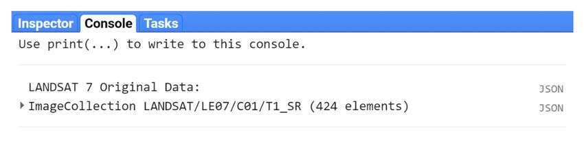
Open Water Journal – Volume 7, Issue 1, Article 4 6
 Example code that selects the Landsat 7 Tier 1 surface reflectance data and filters it by the spatial location is
shown in Figure 2.

 Figure 2. Code to create an image collection labeled “L7” of Landsat 7 images that
 contain Utah Lake.

 Figure 1: Console output presenting information on the resulting image collection,
 consisting of 424 Landsat 7 images of Utah Lake.

 The result is an image collection containing only the images from Landsat 7 at the location we selected. For
our location, Utah Lake, this collection contains 424 images. In the last line of code shown in Figure 2, we print
the results of this process, which is a description and metadata associated with our new image collection to the
console shown in Figure 3, so we can view the description and verify that we selected the correct images. The
interface allows selection of the image collection listing shown in Figure 3 to look at metadata describing for each
image in the collection .
 Each image in the L7 collection we created contains 7 different spectral bands which can be processed to infer
information about the water level, cloud cover, and chl-a concentrations of the lake at the time the image was
taken. For our case study, we only process the images to estimate chl-a concentrations. In addition to the spectral
bands, which were measured by the satellite, each image contains other bands such as the QA/QC band previously
discussed.
2.4 Chl-a Concentration Function
 Next, we processed each image in the L7 collection by using an empirical model to exclude all pixels except
those representing water in Utah Lake and removing the pixels that have quality issues. After masking off pixels
that do not represent lake pixels, we used an empirical equation to estimate chl-a concentrations for the remaining
pixels. To perform these tasks, we created a set of functions which pass over each image in the L7 image collection
and generate results for each image. These results are stored in a new collection of images that represents the chl-
a concentration of Utah Lake over time. The following sections detail each of these steps.

© Copyright owned by the authors unless otherwise noted. OpenWaterJournal.org

Open Water Journal – Volume 7, Issue 1, Article 4 7
2.4.1 Land Mask
 Only water pixels should be analyzed for chl-a concentration, so it is necessary to “mask,” or exclude, land
pixels from each image. To perform this masking, we first manually created a polygon outlining the general area
of the lake using GEE’s geometry tool. This polygon is shown in Figure 4. The code, shown in Figure 5, then
clips the larger Landsat image to this polygon area. Further calculations will only be performed on those pixels
inside the polygon.

 Figure 4. Rough polygon to outline the water body and to roughly select the pixels
 that represent Utah Lake.

 Figure 5. Code to preserve only the image pixels inside the polygon shown in
 Figure 4.

 To refine this selection, we needed to differentiate between the water and land within the polygon. To separate
water pixels from those that contain land, we used the Modified Normalized Difference Water Index (MNDWI)
(Donchyts et al., 2016; Gulácsi & Kovács, 2020; Singh et al., 2015; Sun et al., 2012; Szabó et al., 2020). The
MNDWI classifies pixels containing water, and it works even in the lake areas that have high algal growth (Rokni
et al., 2014; Tate, 2019). The MNDWI algorithm uses the green and first short-wave infrared (SWIR1) bands to
differentiate between the water and land within the polygon. The equation for the MNDWI in terms of the green
and first short-wave infrared (SWIR1) bands is:The MNDWI classifies pixels containing water, and it works even
in the lake areas that have high algal growth (Rokni et al., 2014; Tate, 2019). The MNDWI algorithm uses the
green and first short-wave infrared (SWIR1) bands to differentiate between the water and land within the polygon.
The equation for the MNDWI in terms of the green and first short-wave infrared (SWIR1) bands is:

 Green − SWIR1 Eq 1
 MNDWI =
 Green + SWIR1

© Copyright owned by the authors unless otherwise noted. OpenWaterJournal.org

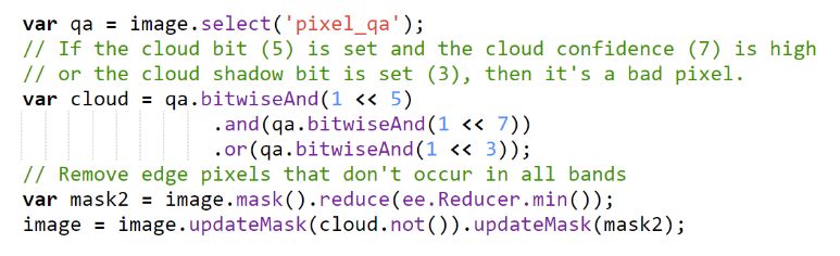
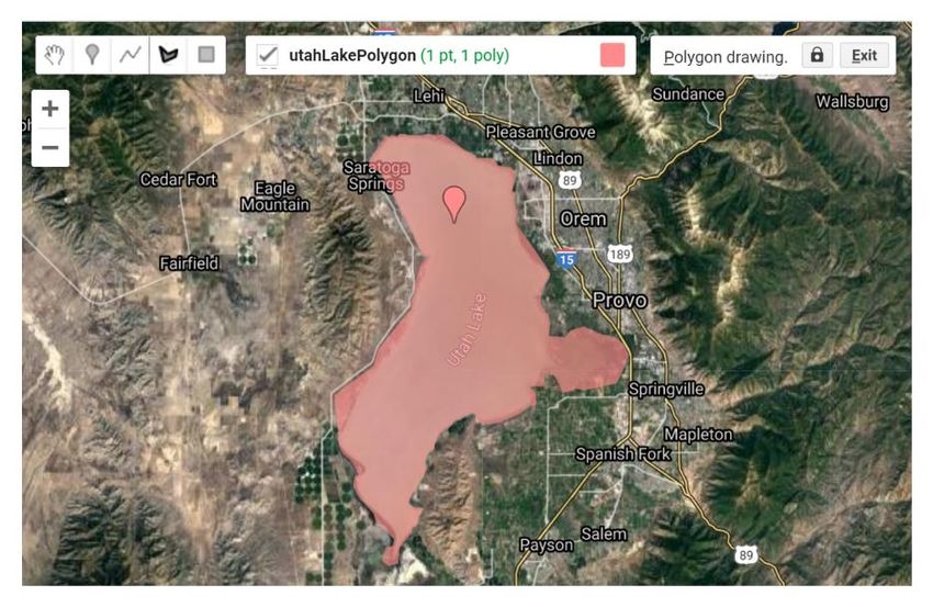
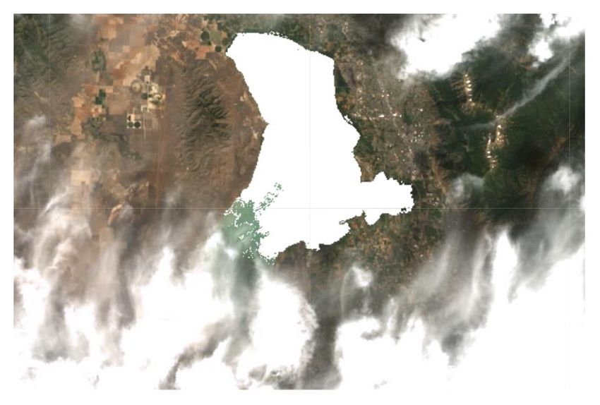
Open Water Journal – Volume 7, Issue 1, Article 4 8
 In GEE, to mask the pixels representing land (land mask) we applied the MNDWI expression to each image,
only using the pixels within the spatial polygon. We then created the land mask by selecting the pixels that have
a MNDWI value greater than 0.95 (i.e., are not water). We selected the threshold of 0.95 based on visual analysis
of a small number of images. The code to generate this mask is shown in Figure 6, where B2 is the band in the
green spectral region and B5 is the first SWIR band; these are Landsat 7 bands 2 and 5, respectively.

 Figure 6. Creating and applying a land mask.

 The function produces a land mask for each image with values of 1 and 0 for pixels representing water and
land, respectively. The result is a “dynamic shoreline” where the lake boundary can change with each image
because each image now consists only of pixels representing water on the day the image was acquired. The extent
of Utah Lake changes over time because of water level changes. Using this MNDWI approach, we can determine
which pixels makeup the lake area for each image in the time history. Figure 7 shows an example of this mask
for a specific image, in this image the white pixels represent water and are included in further analysis. Other
water bodies in the image, such as rivers and ponds, are excluded by the rough polygon we drew around the lake.

 Figure 7. Image showing the computed water mask for the image. The white pixels
 represent the areas with water and are included in the analysis. The other pixels are
 masked from the analysis.

2.4.2 Pixel Quality Mask
 We applied a pixel quality mask to eliminate cloudy and other pixels with poor data from analysis. The Level
2, Tier 1 Landsat data includes a band that has a pixel quality value. This band consists of several different
integers, each representing a different quality issue. Figure 8 presents the code we used to mask out pixels

© Copyright owned by the authors unless otherwise noted. OpenWaterJournal.org

Open Water Journal – Volume 7, Issue 1, Article 4 9
contaminated by clouds or clouds shadows. We used the following bits: bit 5 to represent clouds, bit 7 to represent
cloud confidence, and bit 3 to represent cloud shadows or pixel saturation. The code can be read to say: if bits 5
and 7 are set, i.e., there are clouds and confidence in there being clouds is high, or if bit 3 is set, i.e., there is a
cloud shadow, then mask the pixel. Figure 9 shows an example of an image that includes both a water mask and
a quality mask. Only the solid white pixels are used in the calculation—those obscured by clouds or land are not
included as they have been masked. The image shows how this approach masks even wispy clouds in the bottom
portion of the Lake. While we can “see” water in these pixels, the spectral signature is contaminated with clouds
and is not used in the calculations.

 Figure 8. Pixel quality mask code based on a tutorial provided by Google Earth
 Engine. (https://developers.google.com/earth-
 engine/datasets/catalog/LANDSAT_LE07_C01_T1_SR)

 Figure 9. A cloud masked image. The “white” pixels are used in further
 calculations, the other pixels have been masked from consideration. This image
 also includes the spatial mask, the water mask, and the quality mask.

2.4.3 Computing Algae Concentrations
 Algal concentrations can be estimated by measuring the concentration of chl-a, the green pigment in plants,
present in the water. Remotely measured surface reflectance data can be used to estimate chl-a concentrations by
developing an empirical model that relates image band intensities to the unique spectral signature of chl-a (Hansen
& Williams, 2018). We applied a chl-a concentrations model taken from the literature that was developed for
Utah lake. This model consists of a mathematical expression that uses various image bands from the Landsat data.
The chl-a model we used for this case study was the late season model of Utah Lake from (Hansen & Williams,
2018). The model is presented in Equation 2. Algal concentrations can be estimated by measuring the

© Copyright owned by the authors unless otherwise noted. OpenWaterJournal.org

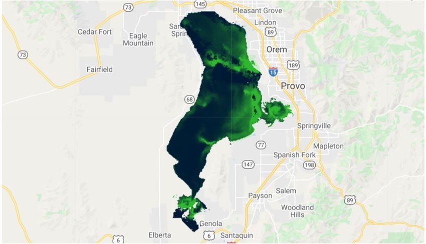
Open Water Journal – Volume 7, Issue 1, Article 4 10
concentration of chl-a, the green pigment in plants, present in the water. Remotely measured surface reflectance
data can be used to estimate chl-a concentrations by developing an empirical model that relates image band
intensities to the unique spectral signature of chl-a (Hansen & Williams, 2018). We applied a chl-a concentrations
model taken from the literature that was developed for Utah lake. This model consists of a mathematical
expression that uses various image bands from the Landsat data. The chl-a model we used for this case study was
the late season model of Utah Lake from (Hansen & Williams, 2018). The model is presented in Equation 2.

 2 3 Eq 2
 chl-a = (7.33−0.004b1−0.05b7+0.01b5)

 The result of applying this equation to the bands of a pixel in an image is the estimated concentration of chl-a
in µg/L for each pixel. Figure 10 shows the code to implement this model, while Figure 11 graphically shows the
results. In this image chl-a concentrations range from low to high represented by the dark-blue and green pixels,
respectively. The image also shows pixels not included in the calculations because of quality issues, mostly
clouds, these pixels are shown in light blue.

 Figure 10. Code to apply the chl-a model.

 Figure 11. A visual representation of the chl-a concentration in an image with dark-
 blue or black representing low chl-a concentration and light green representing high
 concentrations. The light blue area in the bottom of the lake are pixels not included
 in the computation because of quality issues, mostly clouds.

© Copyright owned by the authors unless otherwise noted. OpenWaterJournal.org

Open Water Journal – Volume 7, Issue 1, Article 4 11
2.4.4 Preserving Timestamps
 A small but important coding step necessary to analyze and evaluate chl-a trends is the preservation of
timestamps, which would otherwise be lost in processing. This is done by creating a new property for the new
image that contains the chl-a data that is identical to the Landsat image’s ‘system:time_start’ property. For ease
of use, we kept the time in the same format as the parent ‘system:time_start’ property. This format can also be
converted to a more standard year-month-day format for convenience. The code to preserve the time stamp and
convert it to a standard form is shown in Figure 12.

 Figure 12. Image timestamp preservation.

2.5 Analyzing Trends/Statistical Tests
 The main goal of this project is to identify and quantify the trends in algal concentrations over the study period.
We used the nonparametric Mann-Kendall test to determine the magnitude and sign of the trends for each pixel,
as well as the statistical significance of those trends (Hamed, 2009; Helsel & Hirsch, 1992; Mann, 1945b). We
adapted code from GEE documentation to perform these calculations (Google Earth Engine Tutorials, Non-
Parametric Trend Analysis). Unfortunately, due to the processing time and memory limits on Google’s Servers,
GEE was not able to process the entire time series, so the case study, presented later, uses a limited number of
images. These limits exist because we are using the free version of Google Earth Engine.
 The Mann-Kendall test is commonly employed to detect monotonic trends in series of environmental data and
is recommended by the US EPA National Nonpoint Source Monitoring Program (Meals et al., 2011). The
following discussion follows the EPA guidance (Meals et al., 2011).
 For the Mann-Kendall test, the null hypothesis, H0, is that the data come from a population with independent
realizations and are identically distributed. The alternative hypothesis, HA, is that the data follow a monotonic
trend.
 The Mann-Kendall test statistic is calculated according to:
 −1 

 = ∑ ∑ ( − ) Eq 3
 =1 = +1

 With:
 1 > 0
 ( ) = { 0 = 0 Eq 4
 −1 < 0
 When S is a large positive number, later-measured values tend to be larger than earlier values and an upward
trend is indicated. When S is a large negative number, later values tend to be smaller than earlier values and a
downward trend is indicated. When the absolute value of S is small, no trend is indicated.
 The test statistic, to determine if the indicated trend is statistically significant, is computed as:

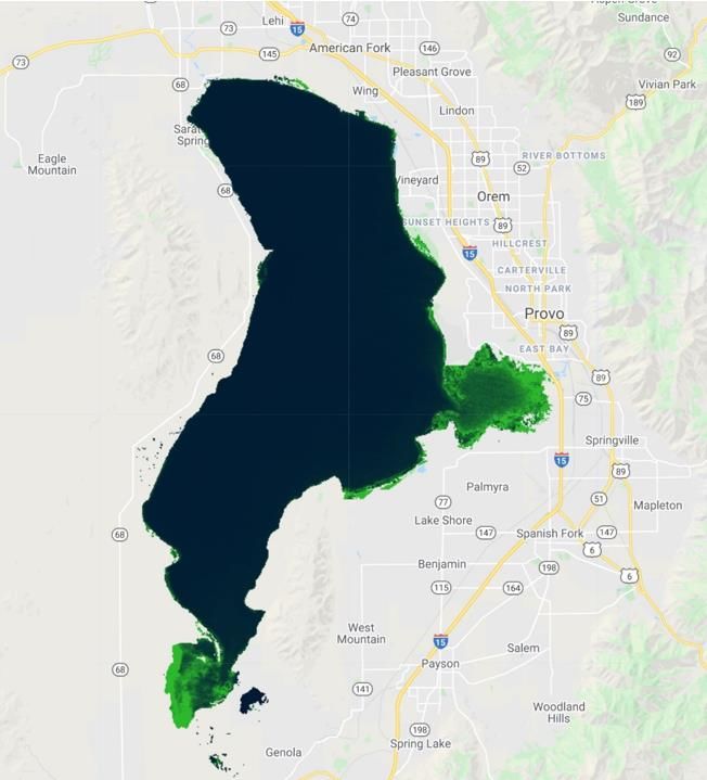
© Copyright owned by the authors unless otherwise noted. OpenWaterJournal.org

Open Water Journal – Volume 7, Issue 1, Article 4 12
 
 = Eq 5
 ( − 1)⁄
 2
which has a range of –1 to +1 and is similar to the correlation coefficient. computed in regression analysis (Meals
et al., 2011). The null hypothesis of no trend is rejected when S and τ are significantly different from zero.
 If a significant trend is found, the rate of change can be estimated using the Sen slope estimator (Helsel &
Hirsch, 1992):
 − 
 1 = ( ) Eq 6
 − 
for all i < j and i = 1, 2, …, n-1 and j = 2, 3,…, n. The Sen slope estimator is the median slope for all data pairs
used to compute S. The slope can also be estimated using standard linear least squares analysis.
 The Mann-Kendall test statistics are invariant to transformations such as logs (i.e., the test statistics will be the
same value for both raw and log-transformed data), the test does not require the data to be evenly spaced and
makes no assumptions on the distribution of the data, so it is applicable in many situations.
3.0 Results
3.1 Overview
 While we will only present results for a limited set of images for most analysis examples in this case study.
We computed the chl-a concentration in each pixel of each image for the entire time series in the Landsat
collection using the process described in section 2.4.3 above. This data set consisted of 1,003 images over a 37-
year period. However, due to processing constraints, we were limited in the number of images we could process
for the Mann-Kendall parameters, as this is a computationally intensive calculation. Using trial and error, we
found that we could only compute the Mann-Kendall results for about 30 images. For the Mann-Kendall analysis
we decided to process the July images from 1999-2015, which represent 16 years of data and contains 31 images.
We selected the July data for this case study as this time of the year has traditionally had large algal blooms. This
time of year is the height of the algal growing season and is of concern to water quality managers and regulators.
In the example figures in this section we will use data from this limited period. We do show all the data in a time
series plot of the median chl-a concentration for the lake. For the remainder of the analysis examples, we show
results for the shorter period.
3.2 Algae concentrations
 We used equation 2 (Section 2.4.3) to calculate the chl-a concentration for each pixel in the 1,003 images
acquired of Utah Lake by the three Landsat mission from 1984 to 2021. These calculations resulted in a set of
images that represent the chl-a concentration spatial distribution on a given date. These images are geo-referenced
and scaled, which means that we can compare the results at a single spatial location over time and compute
statistics for each pixel such as average, median, or standard deviation values for the chl-a data.
 Figure 13 is example that shows the spatial chl-a concentration distribution for March 29, 2013. In this image,
the light green and black representing high and low chl-a concentrations, respectively. These results show that on
March 29, 2013, Provo Bay on the central east side of the lake, and the region around Provo Harbor (near the
outlet of the bay), exhibited high chl-a concentrations. Just north of this area, there is an algal bloom that extends
from the east shore to the west shore. There is also an extensive bloom in Goshen Bay at the south end of the lake.
While maps of the spatial distribution of chl-a concentrations are very useful, they do not provide insight into

© Copyright owned by the authors unless otherwise noted. OpenWaterJournal.org

Open Water Journal – Volume 7, Issue 1, Article 4 13
long-term trends or typical lake conditions, but rather snap shots of the spatial distribution at a given point in
time.

 Figure 13. Algae concentrations in Utah Lake for March 29, 2013.

 We used GEE tools to summarize the data. There are various statistics or other methods available. Figure 14
represents the data summarized as median chl-a concentration values in Utah Lake from 1984-2021 shown as a
line graph. This graph presents water quality over the entire lake over the entire 37-year data set. Figure 14 has a
data point approximately every 16 days during the growing season. In some cases, there is less time between
images because of overlap between the satellites, and the graph does not include data from November, December,
January, or February, as there is little algae during these months and ice or snow results in unreliable estimates.
Any given image most likely has pixels that are masked because of clouds, being outside the lake on that date
(e.g., soil pixels), or have other quality issues. There may be complete cloud cover for some images, meaning
these data are also not included. These masked pixels are not included in the calculation of the median value for
that date. If all the data for a given date is missing, the graph linearly connects the data points on either side. This
can happen when clouds cover the region. In Figure 14, each point on the graph represents the median value for
an entire lake. Graphs such as this provide managers with a better understanding of the lake processes and how
they change over time. While we could not run the Mann-Kendall test of the data in each individual pixel, we did
run the Mann-Kendall test on the data shown in the graph. While visually there is a slight apparent upward trend
in the graph, the Mann-Kendall results indicate this trend is not statistically significant. These data show that algal
concentrations typically peak in July, which is why we selected July data for the other examples. This is an
example of the types of information that can be obtained from this analysis.

© Copyright owned by the authors unless otherwise noted. OpenWaterJournal.org

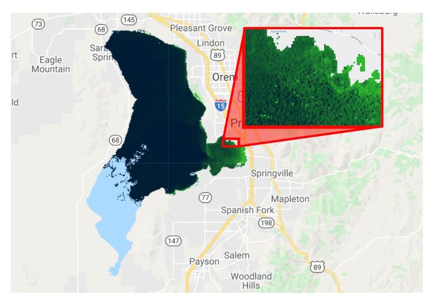
Open Water Journal – Volume 7, Issue 1, Article 4 14

 Figure 14 Median chl-a values for the entire Utah Lake from 1984–2021. This
 chart does not include data for November, December, January, or February. The
 figure shows that chl-a levels typically peak in July, just after the tic-mark.

 Figure 15 shows another way to evaluate the data. It presents the median chl-a concentration in each pixel over
the shorter 16-year test period using data from the month of July. In most years, this is two data points per year,
but in some years, it is only one. This visualization can help answer some of the questions raised by Figure 12,
such as whether the regions west of Orem or the Goshen Bay area generally have higher chl-a concentrations than
the rest of the lake, or whether this spatial distribution only representative of that day. Figure 15 shows that, in
the month of July, both Provo Bay and Goshen Bay typically do have algal blooms. However, this is not the
condition for the remainder of the lake, the bloom shown in the top third of Figure 12 that crosses the lake is not
the average condition. Figure 15 shows that except for Provo Bay and Goshen bay, the remainder of the lake does
not exhibit high median chl-a concentrations over the month of July. Figure 15 shows that there are shoreline
areas that do exhibit high median chl-a values, but this might be the result of having only a few data points because
these pixels are very near the shore, they may not be classified as water pixels in many of the images leaving only
a minimum number of images to compute the median. The high median chl-a values in these shore-line pixels
might also be the result of part of the pixel including shoreline plants. For lake management, these data would
need additional analysis before managers could conclude that these areas typically have blooms in July.

© Copyright owned by the authors unless otherwise noted. OpenWaterJournal.org

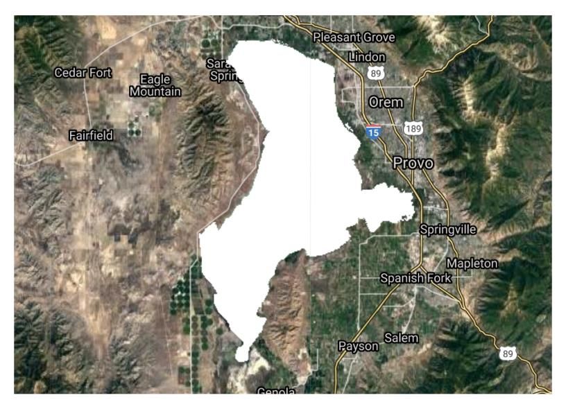
Open Water Journal – Volume 7, Issue 1, Article 4 15

 Figure 15 The spatial distribution of median chl-a values for July during the period
 from 1999-2015. This map presents the median chl-a concentration of 31 images.

3.3 Algae Concentration Trend Analysis
 Figure 16 visualizes the chl-a trend over the 16-year period for the month of July, as determined by the 31
images used in the analysis. This visualization demonstrates the power of using this approach and GEE to better
understand the trends in algal growth in Utah Lake. Figure 16, Panel (a) shows the sign of the chl-a trend’s slope
for the July chl-a concentrations across the 16-year period, with green and red representing positive and negative
slopes, respectively. Figure 16, Panel (b) shows the magnitude of the trend or slope, with blue and red representing
maximum negative and maximum positive trends of -0.1 and +0.1, respectively. Figure 16, Panel (c) indicates
which pixels have statistically significant trends, with white and black pixels representing a statistically significant
and non-statistically significant trends, respectively. This figure shows that in general, pixels with the largest
apparent upward or downward trend were more likely to be statistically significant. However, there are areas in
which pixels with smaller slopes also demonstrated statistical significance.

© Copyright owned by the authors unless otherwise noted. OpenWaterJournal.org

Open Water Journal – Volume 7, Issue 1, Article 4 16

 Figure 16. Chl-a trend maps for July images from 1999-2000. Panel (a) presents
 data trends, with red representing decreasing trends and green increasing; panel (b)
 indicates the magnitude or slope of the trend with greens and yellows indicating
 little to no slope significance, blue and orange indicating a slight down or upward
 slope, and dark blue or red indicating large downward or upward slopes,
 respectively; panel (c) presents the areas of the lake with statistically significant
 trends for July over the 20 year period, with only Provo Bay and Goshen By
 showing any statistically significant trends. In general, these correlate with areas of
 larger downward or upward slopes, but not exclusively.

 Though based on a limited amount of data, the results in Panel (c) of Figure 16 show that there is no statistically
significant trend for the majority of the lake. The Provo Bay region (middle right area) has a large positive trend
in algal growth shown in Panel (b) and the trend is statistically significant as shown in Panel (c). This means that
those areas of Provo Bay have increasingly higher chl-a concentrations during the month of July in recent years,
compared to the early 2000s.

4. Conclusion
 We have presented GEE tools that generates a time history of algal concentrations in Utah Lake using Landsat
data. We collected Landsat surface reflectance images of Utah Lake and identified the water pixels with no quality
issues. We used an empirical model to estimate the chl-a concentration in each of these suitable pixels. In the case
study for Utah Lake, we presented several ways these data could be analyzed, including single maps representing
the spatial distribution of chl-a concentrations at a single point in time, a time-series graph showing how the
median chl-a concentration for the entire lake changed over time, an image of the spatial distribution of median
chl-a concentrations over a selected time period , and the results of applying the nonparametric Mann-Kendall

© Copyright owned by the authors unless otherwise noted. OpenWaterJournal.org

Open Water Journal – Volume 7, Issue 1, Article 4 17
test to a time series of spatial distribution images that identify which pixels showed increasing or decreasing, or
no trends; the magnitude of these trends; and if these trends are statistically significant.
 This tool and analysis approach is applicable to other satellites and lakes or regions, though the empirical
models may need to be adjusted to each lake. For our case study, we implemented an empirical equation from the
literature to estimate chl-a concentrations, using the Level 2 Landsat surface reflectance data. For the case study,
we used a sub-set of 31 July images from 1999 to 2015(Hansen & Williams, 2018). For the case study, we used
a sub-set of 31 July images from 1999 to 2020 to demonstrate the application of the Mann-Kendall nonparametric
test to determine a general trend in algal growth. The test indicated an upward trend in Provo Bay, but given this
limited amount of data, there are some uncertainties in the results.
 Once we can run this process over the entire 40-year image collection, we can better understand water quality
trends on Utah Lake and how various inflows might be affecting lake processes. We are currently working to
implement this functionality. It appears that we may need to implement the algorithms through another GEE
interface.
 Additional goals for future extensions for this project include:
 • Modifying the Landsat 7-pixel data to use infilling to estimate pixel values for pixels affected by the
 2003 Scan Line Corrector failure;
 • Applying season-specific chl-a models to the images, as recommended by Hansen and Williams
 (2018);
 • Using statistical significance results as a mask for other statistical results so that only statistically
 significant trend results are mapped, for example the map that shows trend magnitude would only
 include data for pixels that demonstrated a statistically significant trend;
 • Develop a method to apply the Mann-Kendall test to the entire dataset, either by fitting computation
 within allotted space on Google servers or by performing computation in a local environment; and
 • Validating our estimated chl-a concentrations against coincident field data
Acknowledgements
 This research was supported in part through the Utah NASA Space Grant Consortium, NASA Grant #
80NSSC20M0103, the BYU College of Engineering Freshman Fellowship Program, and the Cardall and Tanner
parental scholarship funds.
Software Availability
 The GEE code described in this paper is available on request. It is somewhat disorganized and not easy to
follow. Each of the functions described in this paper are fully implemented in the code, however, the code is not
designed or coded to be production ready. Each capability in the code is relatively “stand alone”; the code is not
integrated to provide a seamless tool for computing chl-a trends. For example, the code creates a complete image
collection of all the useable Landsat images from 1984 to the present. However, the Mann-Kendall code, as
discussed above, can only process a limited number of images. The code to select this subset of images, while
working well, is not well suited for regular use.
References
Allan, M. G., Hamilton, D. P., Hicks, B., & Brabyn, L. (2015). Empirical and semi-analytical chlorophyll a
 algorithms for multi-temporal monitoring of New Zealand lakes using Landsat. Environmental monitoring
 and assessment, 187(6), 1-24.

© Copyright owned by the authors unless otherwise noted. OpenWaterJournal.org

Open Water Journal – Volume 7, Issue 1, Article 4 18
Bonansea, M., Rodriguez, M. C., Pinotti, L., & Ferrero, S. (2015). Using multi-temporal Landsat imagery and
 linear mixed models for assessing water quality parameters in Río Tercero reservoir (Argentina). Remote
 sensing of Environment, 158, 28-41.
Brivio, P. A., Giardino, C., & Zilioli, E. (2001a). Determination of chlorophyll concentration changes in Lake
 Garda using an image-based radiative transfer code for Landsat TM images. International Journal of
 Remote Sensing, 22(2-3), 487-502.
Brivio, P. A., Giardino, C., & Zilioli, E. (2001b). Validation of satellite data for quality assurance in lake
 monitoring applications. Science of the total environment, 268(1-3), 3-18.
Castenholz, R. W. (1960). Seasonal changes in the attached algae of freshwater and saline lakes in the lower grand
 coulee, washington. Limnology and Oceanography, 5(1), 1-28.
Donchyts, G., Schellekens, J., Winsemius, H., Eisemann, E., & Van de Giesen, N. (2016). A 30 m Resolution
 Surface Water Mask Including Estimation of Positional and Thematic Differences Using Landsat 8,
 SRTM and OpenStreetMap: A Case Study in the Murray-Darling Basin, Australia. Remote Sensing, 8(5),
 386. https://www.mdpi.com/2072-4292/8/5/386
Gulácsi, A., & Kovács, F. (2020). Sentinel-1-Imagery-Based High-Resolution Water Cover Detection on
 Wetlands, Aided by Google Earth Engine. Remote Sensing, 12(10), 1614. https://www.mdpi.com/2072-
 4292/12/10/1614
Hamed, K. (2009). Exact distribution of the Mann–Kendall trend test statistic for persistent data. Journal of
 hydrology, 365(1-2), 86-94.
Hansen, C., Swain, N., Munson, K., Adjei, Z., Williams, G. P., & Miller, W. (2013). Development of sub-seasonal
 remote sensing chlorophyll-a detection models. American Journal of Plant Sciences, 2013.
Hansen, C. H. (2015). Google Earth Engine as a Platform for Making Remote Sensing of Water Resources a
 Reality for Monitoring Inland Waters.
Hansen, C. H., Burian, S. J., Dennison, P. E., & Williams, G. P. (2017). Spatiotemporal variability of lake water
 quality in the context of remote sensing models. Remote Sensing, 9(5), 409.
Hansen, C. H., Burian, S. J., Dennison, P. E., & Williams, G. P. (2020). Evaluating historical trends and influences
 of meteorological and seasonal climate conditions on lake chlorophyll a using remote sensing. Lake and
 Reservoir Management, 36(1), 45-63.
Hansen, C. H., & Williams, G. P. (2018). Evaluating Remote Sensing Model Specification Methods for
 Estimating Water Quality in Optically Diverse Lakes throughout the Growing Season. Hydrology, 5(4).
Hansen, C. H., Williams, G. P., & Adjei, Z. (2015). Long-term application of remote sensing chlorophyll detection
 models: Jordanelle Reservoir case study. Natural Resources, 6(02), 123.
Hansen, C. H., Williams, G. P., Adjei, Z., Barlow, A., Nelson, E. J., & Miller, A. W. (2015). Reservoir water
 quality monitoring using remote sensing with seasonal models: case study of five central-Utah reservoirs.
 Lake and Reservoir Management, 31(3), 225-240.
Helsel, D. R., & Hirsch, R. M. (1992). Statistical methods in water resources (Vol. 49): Elsevier.

© Copyright owned by the authors unless otherwise noted. OpenWaterJournal.org

Open Water Journal – Volume 7, Issue 1, Article 4 19
Ho, J. C., Stumpf, R. P., Bridgeman, T. B., & Michalak, A. M. (2017). Using Landsat to extend the historical
 record of lacustrine phytoplankton blooms: a Lake Erie case study. Remote sensing of Environment, 191,
 273-285.
Klemas, V. (2012). Remote sensing of algal blooms: an overview with case studies. Journal of Coastal Research,
 28(1A), 34-43.
Landsat—Earth observation satellites. (2015-3081). (2016). Reston, VA: U.S. Geological Survey Retrieved from
 http://pubs.er.usgs.gov/publication/fs20153081.

Ma, R., & Dai, J. (2005). Investigation of chlorophyll‐a and total suspended matter concentrations using Landsat
 ETM and field spectral measurement in Taihu Lake, China. International Journal of Remote Sensing,
 26(13), 2779-2795.
Mann, H. B. (1945a). Nonparametric Tests Against Trend. Econometrica, 13(3), 245.
Mann, H. B. (1945b). Nonparametric Tests Against Trend. Econometrica, 13(3), 245-259.
 http://www.jstor.org/stable/1907187
Masek, J. G., Vermote, E. F., Saleous, N. E., Wolfe, R., Hall, F. G., Huemmrich, K. F., et al. (2006). A Landsat
 surface reflectance dataset for North America, 1990-2000. IEEE Geoscience and Remote Sensing Letters,
 3(1), 68-72.
Mayo, M., Gitelson, A., Yacobi, Y., & Ben-Avraham, Z. (1995). Chlorophyll distribution in lake Kinneret
 determined from Landsat Thematic Mapper data. Remote Sensing, 16(1), 175-182.
Meals, D. W., Spooner, J., Dressing, S. A., & Harcum, J. B. (2011). Statistical analysis for monotonic trends.
 (Tech Notes 6). Fairfax, VA: U.S. Environmental Protection Agency Retrieved from
 https://www.epa.gov/polluted-runoff-nonpoint-source-pollution/nonpoint-source-monitoringtechnical-
 notes.
Nelson, S. A. C., Soranno, P. A., Cheruvelil, K. S., Batzli, S. A., & Skole, D. L. (2003). Regional assessment of
 lake water clarity using satellite remote sensing. Journal of Limnology, 62(1s), 27.
Olmanson, L. G., Bauer, M. E., & Brezonik, P. L. (2008). A 20-year Landsat water clarity census of Minnesota's
 10,000 lakes. Remote sensing of Environment, 112(11), 4086-4097.
Olsen, J., Williams, G., Miller, A., & Merritt, L. (2018). Measuring and Calculating Current Atmospheric
 Phosphorous and Nitrogen Loadings to Utah Lake Using Field Samples and Geostatistical Analysis.
 Hydrology, 5(3), 45. https://doi.org/10.3390/hydrology5030045
Randall, M. C., Carling, G. T., Dastrup, D. B., Miller, T., Nelson, S. T., Rey, K. A., et al. (2019). Sediment
 potentially controls in-lake phosphorus cycling and harmful cyanobacteria in shallow, eutrophic Utah
 Lake. PloS one(2). https://journals.plos.org/plosone/article?id=10.1371/journal.pone.0212238
Richardson, L. L. (1996). Remote sensing of algal bloom dynamics. BioScience, 46(7), 492-501.

© Copyright owned by the authors unless otherwise noted. OpenWaterJournal.org

Open Water Journal – Volume 7, Issue 1, Article 4 20
Robert M Cox Jr, Forsythe, R. D., Vaughan, G. E., & Olmsted, L. L. (1998). Assessing water quality in Catawba
 River reservoirs using Landsat thematic mapper satellite data. Lake and Reservoir Management, 14(4),
 405-416.
Rokni, K., Ahmad, A., Selamat, A., & Hazini, S. (2014). Water Feature Extraction and Change Detection Using
 Multitemporal Landsat Imagery. Remote Sensing, 6(5), 4173-4189. https://www.mdpi.com/2072-
 4292/6/5/4173
Singh, K. V., Setia, R., Sahoo, S., Prasad, A., & Pateriya, B. (2015). Evaluation of NDWI and MNDWI for
 assessment of waterlogging by integrating digital elevation model and groundwater level. Geocarto
 International, 30(6), 650-661.
Strong, A. E. (1974). Remote sensing of algal blooms by aircraft and satellite in Lake Erie and Utah Lake. Remote
 sensing of Environment, 3(2), 99-107.
Stumpf, R. P. (2001). Applications of satellite ocean color sensors for monitoring and predicting harmful algal
 blooms. Human and Ecological Risk Assessment: An International Journal, 7(5), 1363-1368.
Sun, F., Sun, W., Chen, J., & Gong, P. (2012). Comparison and improvement of methods for identifying
 waterbodies in remotely sensed imagery. International Journal of Remote Sensing, 33(21), 6854-6875.
Szabó, L., Deák, B., Bíró, T., Dyke, G. J., & Szabó, S. (2020). NDVI as a Proxy for Estimating Sedimentation
 and Vegetation Spread in Artificial Lakes—Monitoring of Spatial and Temporal Changes by Using
 Satellite Images Overarching Three Decades. Remote Sensing, 12(9), 1468. https://www.mdpi.com/2072-
 4292/12/9/1468
Tate, R. S. (2019). Landsat Collections Reveal Long-Term Algal Bloom Hot Spots of Utah Lake.
U. S. Census Bureau Administration, C. S. D. (2011). US Census Bureau Publications - Census of Population and
 Housing. In.
Wheeler, S. M., Morrissey, L. A., Levine, S. N., Livingston, G. P., & Vincent, W. F. (2012). Mapping
 cyanobacterial blooms in Lake Champlain's Missisquoi Bay using QuickBird and MERIS satellite data.
 Journal of Great Lakes Research, 38, 68-75.
Williams, G. P., Casbeer, W., Nelson, E. J., & Borup, B. (2010, 2010-05-14). Phosphorus Distribution in
 Reservoir Sediments: Implications for Groundwater Transport. Paper presented at the World
 Environmental and Water Resources Congress 2010.
Yip, H., Johansson, J., & Hudson, J. (2015). A 29-year assessment of the water clarity and chlorophyll-a
 concentration of a large reservoir: Investigating spatial and temporal changes using Landsat imagery.
 Journal of Great Lakes Research, 41, 34-44.

© Copyright owned by the authors unless otherwise noted. OpenWaterJournal.org