Tangled String for Multi-Timescale Explanation of Changes in Stock Market - MDPI
←
→
Page content transcription
If your browser does not render page correctly, please read the page content below
Article
Tangled String for Multi-Timescale Explanation of
Changes in Stock Market
Yukio Ohsawa 1,*, Teruaki Hayashi 1 and Takaaki Yoshino 2
 1 School of Engineering, The University of Tokyo, Tokyo 113-8656, Japan; hayashi@sys.t.u-tokyo.ac.jp
 2 Nissei Asset Management Corp., Tokyo 100-8219, Japan; gk13471@ro.bekkoame.ne.jp
 * Correspondence: info@panda.sys.t.u-tokyo.ac.jp; Tel.: +81-3-5841-2908

 Received: 26 January 2019; Accepted: 13 March 2019; Published: 22 March 2019

 Abstract: This work addresses the question of explaining changes in the desired timescales of the
 stock market. Tangled string is a sequence visualization tool wherein a sequence is compared to a
 string and trends in the sequence are compared to the appearance of tangled pills and wires
 bridging the pills in the string. Here, the tangled string is extended and applied to detecting stocks
 that trigger changes and explaining trend changes in the market. Sequential data for 11 years from
 the First Section of the Tokyo Stock Exchange regarding top-10 stocks with weekly increase rates
 are visualized using the tangled string. It was found that the change points obtained by the tangled
 string coincided well with changes in the average prices of listed stocks, and changes in the price of
 each stock are visualized on the string. Thus, changes in stock prices, which vary across a mixture
 of different timescales, could be explained in the time scale corresponding to interest in stock
 analysis. The tangled string was created using a data-driven innovation platform called Innovators
 Marketplace on Data Jackets, and is extended to satisfy data users here, so this study verifies the
 contribution of data market to data-driven innovation.

 Keywords: multi-timescale analysis; change explanation; stock market; data market

1. Introduction: Problem Definition
     Stock analysts are often classified simply into fundamentalists and technical analysts, i.e.,
chartists. The former considers the basic effects of events that significantly affect stock investors’
decisions, whereas the latter analyze charts, i.e., the time series of stock prices. Although these two
groups tend to be regarded differently, it is quite natural that a chartist may also consider the effects
of social events not shown in charts [1] and that a fundamentalist may also refer to sequential data
regarding stock prices [2,3]. The existence of these two approaches is partially analogous to the
positioning of real (human) analysts and machine learning. Machine learning tools have been
recently adopted to forecast market demand [4–7] from data, and this can be regarded as the partial
automation of the thoughts of a technical analyst. However, changes in the market due to external
events are hard to explain by learning from data, because the consideration of external events
indicates that these fundamental causes of investor behaviors are not included in available data. Not
only investors, but also policy-makers related to the market need to explain the changes in the
market resulting from external events.
     The main goal of this study is to enable the detection and the explanation of changes in the stock
market from available sequential data on stock prices. We aim to detect changes in investor
preferences that influence the market and to explain the associated causality, i.e., why investors
showed positive preference for a certain group of stocks, and why the positive attitude was
subsequently overwhelmed by the appearance of a new trend. Here, we define a trend as the
enhancement of various investor preferences for a certain set of stocks for a certain period. We
simply regard the stock market as a place where the trends of investor preferences compete, which

Information 2019, 10, 118; doi:10.3390/info10030118                         www.mdpi.com/journal/information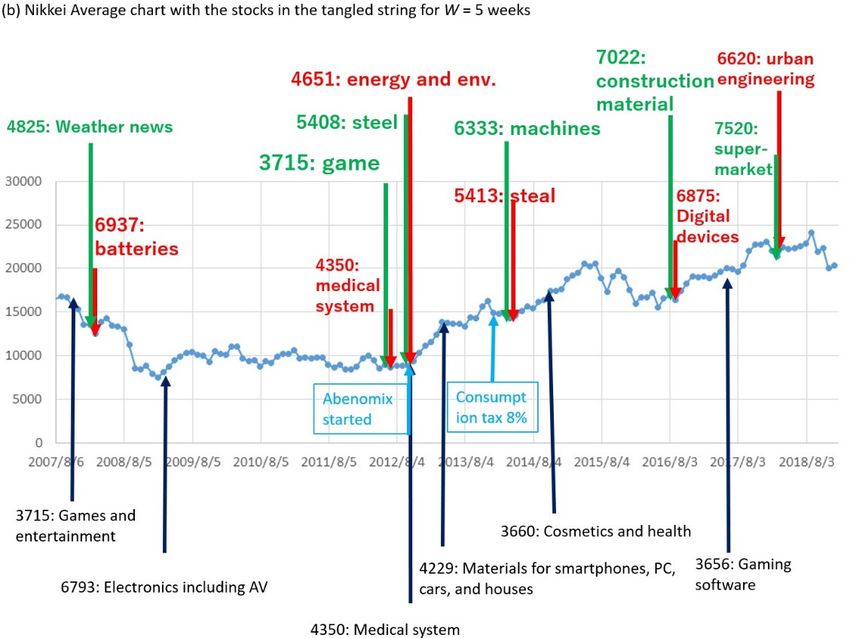
Information 2019, 10, 118                                                                            2 of 21

reflects complex social dynamics because each trend is a mixture of various causalities across
different timescales. On the other hand, negative effects such as the downpricing/disappearance of
stocks, or chained downpricing/bankruptcies are excluded from our scope in order to reduce the
complexity in modeling the interaction of both positive (to buy stocks) and negative (to sell or not to
buy) motivations.
      So far, event studies have been applied to validate the effects of focused information generating
events such earnings announcements or discount rate changes, estimates of earnings, and news events
[8,9] on the changes in stock prices in the period following the events. Machine learning was also
applied for the prediction of changes using the results of event studies as teaching signals [10]. On the
other hand, in this study we aim to aid analysts in the detection and explanation of changes in the
market and in the price of each stock, in such a long-term sequence of 10 years or more. Furthermore,
we aim to enable the explanation based on real and available data that includes events occurring under
the action of several different causalities. Regarding the availability of data, professional analysts
working for asset companies may have elaborate data that are classified into categories of stocks and
also include downpriced stocks that may not be listed anymore in the stock exchange market. We, on
the other hand, use the sequential data on stock prices, which is available to the public, where
timescales are mixed and information about the worst companies are typically unavailable.
      Suppose we have data D on the increase in stock prices designated as { | 0 < ≤ }, where Bt
stands for a basket, i.e., a set of members of itemset I, forming a co-occurring set of top-rank, up-pricing
stocks. D is regarded as the data corresponding to the high-rank preference of investors at time t,
which corresponds to the research interest in the positive preference of investors as mentioned above,
and T is the sequence length of the data. This type of basket data has been used for explaining patterns
and changes in the market [11–13]. For example, suppose the weekly average stock prices of firms in
healthcare businesses show the greatest increase for a month, whereas those in electronics registered a
greater increase last year. The cause of this new trend may be the interest intensified by investors in
healthcare due to a famous movie at the end of the previous year that dealt with the negative effect of
daily foods on human health. This causality may be explained if stock analysts, who broadcasted the
analysis to investors, were also interested in the movie (certainly not in the set I) during the
corresponding period. Furthermore, policy-makers can plan ahead to support healthcare businesses if
the new trend is regarded as sustainable on a long timescale.
      Using machine learning, change points of the features (parameters in parametric models) of time
series models have also been detected. By projecting the data to the principal components, for example,
the sensitivity of change detection was improved using the method for detecting the changes in the
correlation, variance, and mean of the components with time [14]. Changes in model parameters that
capture the structure of the latent causality have been detected in discrete [15–17] and continuous [18]
time series. Here, suppose the changes in the values of the parameter set Θ from time t−δt to t is
learned as Θ [t−Δt, t]−Θ [t−δt−Δt, t−δt], where Δt is the length of the training time of the data to learn Θ
from and δt is the given time step from before (t−δt) to the present (t). The precision of change
detection is expected to improve for larger values of Δt that can be regarded as a part of the tolerant
delay, i.e., the length of time that analysis should wait to detect a change. In [12], the author pointed
out that a large value of Δt is not convenient for capturing the variations accurately. On the other hand,
the focus of this study is to detect events that explain the changes in the timescale that is in accordance
with the interest of the analyst or investor. This corresponds to the detection of change points for δt
that fits the users’ purpose, to relate with external information that can explain the changes in a time
scale corresponding to δt. In machine learning for price forecasting using an adaptive timescale, a
mixture of patterns across various timescales has been fitted to real data to analyze the price dynamics
on different granularities and different abstraction levels and a high accuracy classification into
patterns of decision opportunities in stock investment was realized [7]. On the other hand, in this
paper we aim to aid an analyst’s explanation of a complex, mixed timescale sequence. Like a tangle on
a string (to be illustrated as “a complex part” in Figure 1), the complexity of each subsequence where
the behavior of different investors are mixed may be grasped without separating or reducing into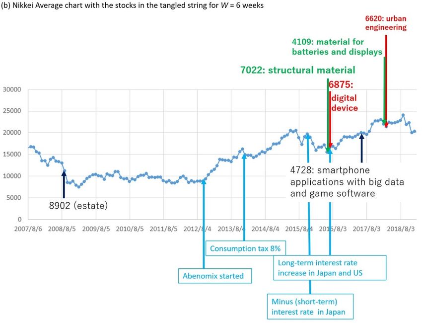
Information 2019, 10, 118                                                                                   3 of 21

simple patterns, as long as the abstract of each complex part and the ending/starting points of each
complex part can be used for explaining the changes in the sequence.

                    Figure 1. Visualization of a sequence by a string with complex tangled parts.

      In order to explain a change, in addition to detecting it, we may consider employing methods to
learn latent topics from sequential data. Consecutive time segments, each of which corresponds to a
vector in the space of a limited dimension of latent topics (without labels corresponding to the
meaning of the topics) are obtained by the dynamic topic model (DTM) [19]. By applying DTM to sales
data, the changes in consumers’ interests can be detected as the boundaries between the obtained time
segments corresponding to discontinuous changes in the topic vector. The topic tracking model (TTM)
has been also presented to analyze the change in each consumer if consumer behavior c is reflected on
the data of Bt,c, instead of Bt above [13]. The hierarchical structure of topics has also been learned [20],
which indicates the potential to explain the changes behind observed events by considering latent
events, i.e., deep causes not covered by the data in hand. On the other hand, we aim to obtain different
explanations where trends (corresponding to topics in the sequence) in the explained scenarios change
at different times, and for different timescales, by introducing external information about latent events.
For example, the sequence of stock prices for a decade can be explained as the shifts in trending
business domains if we think in terms of an annual timescale, but we may observe different change
points such as the effects of analysts’ or firm managers’ predictions if we consider a monthly timescale.
Thus, we regard D as { , | ∈ [1, ], ∈ [1, ]} in place of { | 0 < ≤ } mentioned above, where i
stands for a timescale and Bt is the union of Bi,t for all i in {1, 2, …, n}, where n is the number of mixed
timescales. To further the understanding, the problem here is to obtain {                   , | ∈ [1, ], ∈ [1, ]}
and {      , |  ∈  [1, ], ∈ [1,    ]}, where enti,t and ext i,t represent events at time t that play the role of an
entrance to and exit from a trend in the i-th timescale considered, respectively. If no event at time t
plays the role, enti,t and exti,t should take a null value.
      In this study, for the main goal mentioned above, we consider the subgoal of aiding the human in
linking parts of a sequence that is difficult to explain, to other parts and external information. Here we
assume that an essential part of the difficulty in explanation comes from the complexity of
event-to-event causality, where an event may occur in the mixture of various subsequences. From this
assumption, we extend the tangled string (TS), as in Section 2, which deals with a sequence where
patterns of different timescales coexist. Such a sequence is usual for data on the behavior of
participants in a society who may not share the same interest in topics or trends. Behind the sequence
of stock prices, various investors really have different reasons for buying and/or selling stocks,
reflecting their various interests in the market dynamics in various timescales. In TS, a sequence is
visualized as a string as in Figure 1 where a node and an edge represent an event and the temporal
order of events, respectively, and each tangled part corresponds to a complex mixture of different
subsequences in various timescales corresponding to the different interests of investors if applied to a
stock price sequence shown in Section 2.1. Each tangled part corresponds to a trend of included stocks,
and the multiple paths meet at entrances (stocks A and E) and exits (stocks E and F) of a tangled part,
as stated above regarding enti,t and exti,t. The choice of method for data visualization becomes key for
integrating the approaches of fundamentalist and technical analysts, by providing both classes of (if
we can so classify) investors with links to information that they should refer to via the procedure to be
shown in Section 2.3. For example, a simple stock price chart may turn out to be a useful visualization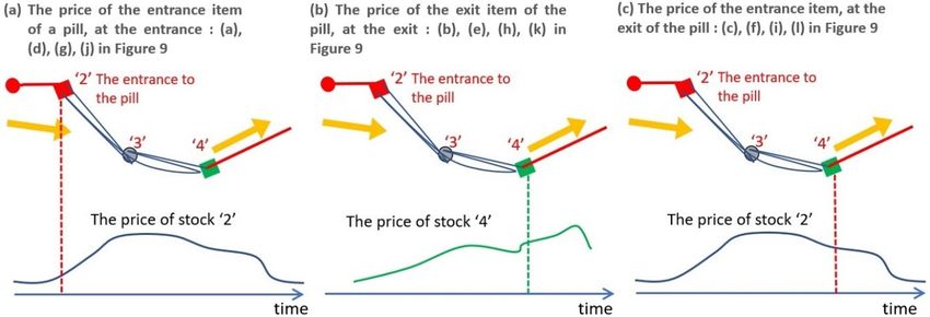
Information 2019, 10, 118 4 of 21
if the essential tipping points of price transition are marked so that an investor can link them with
external information about events affecting the stock market. In addition, the graphical visualization of
the map of stocks and the news provide hints about sentiments in the market relevant to stocks [21,22].
In Section 3, we show the coincidence found in the results of TS with the beginning of the increasing
value of stocks in the market and with major changes in stock prices. In Section 4, we discuss the
qualitative explanations of trend shifts given by stock analysis experts based on the output of TS. The
conclusions relate these results to our future work.
2. TS for a Stock Price Sequence
In this section, we introduce the tangled string (TS hereafter [23,24]) as a method for the
analysis and visualization of sequential data. This tool is expected to fulfill the purpose stated in the
previous section, i.e., to explain the changes in a sequence where different timescales coexist.
2.1. Origins of TS and the Data Market
The original version of TS was a product of the Innovators Marketplace on Data Jackets (IMDJ),
a market-like creativity support system [25,26]. On IMDJ, data providers make available the data
that they have and/or possible methods for data analysis, while data users post requirements for
data and analysis technologies or methods. Events in the given sequential data are analyzed and
visualized by TS as nodes on a string, where the importance of each event is computed according to
their positions on the string. This visualization has been designed to fit the user’ requirements
presented in IMDJ; that is, in order to realize the method M1 below for satisfying the requirement R1.
TS was originally invented for detecting the message with the highest social impact from a log of
human communication (DJ1) by considering the trends of topics in the preceding and subsequent
messages. After choosing such words, additional information about disasters (DJ2) should be used
for validating the credibility of the message corresponding to the chosen messages.
Requirement R1: collect information useful for decision making
Method M1: obtain a high impact message in a sequence and relate it to external information
Data for realizing M1: {DJ1: log text of communication, DJ2: information about disasters}
The performance of TS has been shown to satisfy the requirement R1 above and others in the
analysis of the text in timelines and the sensor-based log of human’s movements in office [23]. After
TS was invented as a response to R1, it came to be required in the following set.
Requirement R2: explain events in the tipping points of consumer behaviors in the market
Method M2: detect a high impact event by TS and relate it with external information to explain
the causality
Data for realizing M2: {DJ3: log of consumptions or purchase history, DJ4: social events and news}
In this paper, we take the stock market as the target market in R2 and investors as consumers.
That is, R2, as listed above, is expected to be solved by TS in this paper (challenged since [24]), by an
analogy from R1, as shown in the Discussions section of this paper, where the detected events are
explained by an expert with links to external information and news such as Prime Minister Abe’s
policy for the national economy. Although the obtained explanation is not guaranteed to be the only
one or the best, we can say that the changes corresponding to the complex parts in the sequence
came to be linked to real social events in the explanations, as illustrated in Figure 1. The novelty here
is that we introduce the analogy from DJ1 (log text of communication) to DJ3 (log of consumptions or
purchase history) and from the relation of requirement(R1)-method(M1)-data(DJ1, DJ2) to
requirement(R2)-method(M2)-data(DJ3, DJ4).
2.2. TS Algorithm
As shown in Figure 1, the tangled string (TS) visualizes a string corresponding to a sequence,
where each complex part corresponds to a tangled substring as in Figure 2. In TS, a sequence is
modeled by a string of which each tangled substring is called a pill. A pill is defined as a sequence of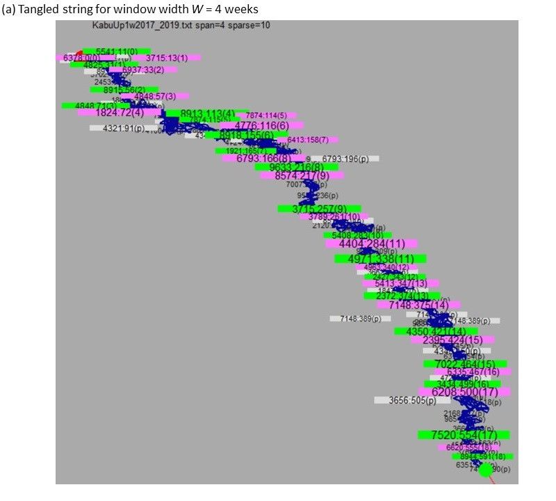
Information 2019, 10, 118 5 of 21
events beginning from a particular event to the appearance of the same event in the sequence. Events
in the sequence are classified into two components: (1) events in pills and (2) others on wires that are
substrings connecting pills.
Figure 2. Tangled string TS applied for String. si is the i-th event in the sequence, corresponding to
the token “x” beside it.
In order to reduce ambiguity, the symbol expressing an event (in this study, the pricing up of a
stock) is called a token. In natural language, the same token may mean different items, and the same
item may be represented by different tokens. On the other hand, the token representing a stock ID (a
number representing a unique stock) is the event that the increase in the stock price ranked in the
top-10 (or top-5, depending on the target data) in the market. Therefore, a token corresponds
uniquely to an event at a certain time in the target sequence. Pills formed in the sequence may meet
each other, due to their sharing the same tokens. As a result, a string having pills may cross itself to
make a larger pill. For example, in Figure 2, the pill including {s2 (=”3”), s3 (=”2”), s4 (=”3”)} and the
pill including {s5 (=”4”), s6 (=”3”)} meet at s2, s4, and s6 because they include the same token “3” and
form one pill. Thus, a pill may include other pills; a maximum pill (a pill not properly included by
any other pill) is called just a pill hereafter. The same token may appear multiple times in a pill
within a constant time window, which means that a pill corresponds to a trend where the included
items appear repeatedly.
On the other hand, events on wires represent the changes from a trend represented by a pill to
the next trend. In this sense, the connections of pills via wires are expected to be used to explain
changes in the sequence. By the connection of pills and wires, we aim to visualize sequential data to
explain the changes in the trends and their causes. The TS algorithm is given below as Algorithm 1.
Algorithm 1. Original version algorithm of TS algorithm (Revised from [23] without changing the meaning)
Initial setting:
String = {s1, …, … si, …sj, …, …, sL},
Wires = {w1-w2-w3-…-wL−1} where wi = si−si+1 represents the edge connecting the adjacent pair of tokens
for i = 1 to L: pill(si) = si where pill(s) represents the pill including event s.
weight(si) = 0
For W, a preset window, execute the cycles below:
For i = W + 1 to L:
Neighbors (si, W) = {si-W, si-W+1, …, …, si-1}
if sj(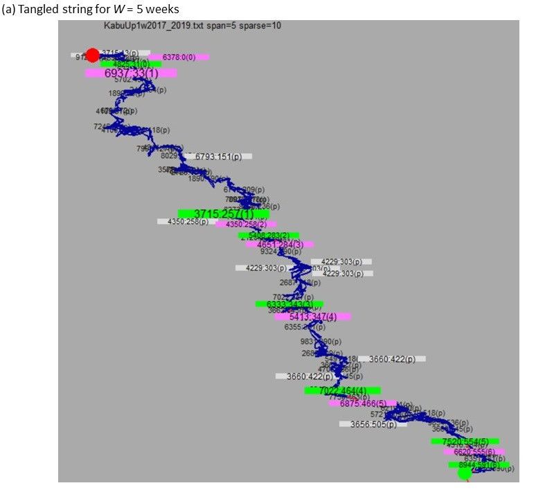
Information 2019, 10, 118                                                                                          6 of 21

      End For
      For each pill
        sent, sext = the first and the last event in pill
        weight(sent) =weight(sext) = ext – ent      # assign the pill size as the weight of each event on a wire
      End For

       Here, si denotes an event that the symbol token(si) appeared at the i-th position in the given
string String, rather than the symbol itself. That is, token(si) is unique to a symbol, and si for multiple
i’s may correspond to the same symbol. In the initial setting, no pill but only a single wire exists as a
string corresponding to the given sequence of length L. After the initial setting, each event si in the
string is considered one by one in the ascending order. For each si, the event sj of the same token as si
is searched from the events preceding si within the window of the time interval W in weeks (e.g., W =
3 implies that the interval is 3 weeks), represented by Neighbors(si) in the backward search for events,
i.e., for the time range [i−W, i−1]. If such an event sj is found, si and all the events between sj and si are
considered to belong to the same pill as sj (i.e., pill(sj) = pill(sj)); so, the trend in this pill appears as
repeated tokens (as token(si) = token(sj)). A pill may later become a part of a larger pill if a token in the
succeeding W baskets matches with a token in the pill. The substring between sj and si is pruned
from Wires, which represents the set of all the wires if sj and si join the same pill. On the other hand, if
no event such as sj for which the token (token(sj)) is equal to token(si) is found within the window of W
baskets before si, then si and all the events in Neighbors(si) stay as a wire. After the cycles, a position
(position i) is assigned to each si.
       When a new event si is added as a node in a pill, the size of the pill is increased by the number of
events added. After all the cycles are completed, the weights of sent and sext, which are the first and
last events (i.e., st of the smallest and the largest t) in each pill, denoted by weight(sent) and weight(sext),
respectively, take the values of the size of the pill. This means that the size of a pill is counted as the
weight loaded on the edges of the wires connected to the pill. We call sent the entrance to the pill and
sext the exit from the pill. The events at the entrance and the exit of a pill are visualized as a red and a
green node, respectively, on the string. Each of these events having a large value of weight is
visualized by a large letter. These events play an important role in explaining the changes in the
trends in the sequence, such as trend shifts in the market. For example, if TS is applied to the
sequence String as Equation (1).
                                     String = 1, 2, 3, 2, 3, 4, 3, 4, 5, 6, 2, 5, 6, 7.                              (1)
      In this case, as shown in Figures 2 and 3a, the event of the appearance of an item represented by
token “2” starts the first pill including itself, along with “3” and “4”, because “2” is the first token
revisited by the other nodes in the string. The first item ”1” in the sequence is assigned to the event
s0, and “2” is to s1 as well as s3. The token “3” is visited thrice, i.e., as {s2, s4, s6}, and “4” is visited twice
as {s5, s7}. In this pill, “4” is the last token repeated, so it is regarded as the exit of the pill. Then “4” is
the beginning of the wire that connects to the next pill. Here, TS visualizes the flow of the sequence,
highlighting the nodes where each wire is connected to the preceding and following pills. Events on
the wires may not look outstanding because they are not frequent in pills that are repeated.
However, an on-wire node possibly plays an essential role in the mainstream of the sequence
because the connection in the whole structure is cut off if such an event is lost. Although in this
sense, the event of token “3” in Figures 2 and 3a may be suitable to be on a wire as the structure gets
destroyed by deleting “3”; here “3” is regarded not as an on-wire, but the main event in the first pill
as the other events in the first pill are connected to “3”.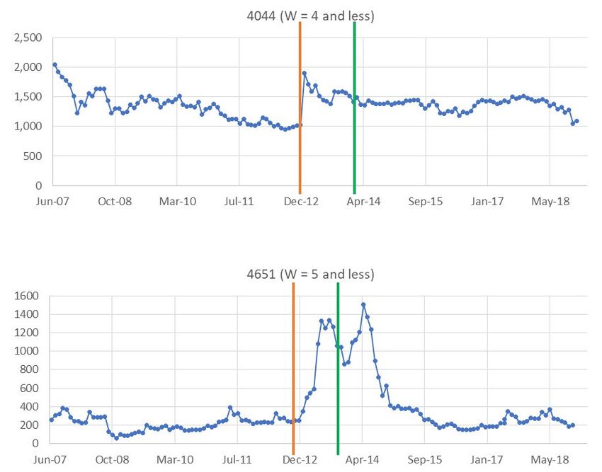
Information 2019, 10, 118 7 of 21
(a) (b)
Figure 3. TS employed for the widths (W) of 6 and 7 (the unit of W is a week). (a) is for W = 6, (b) for W = 7.
The overlapping letters are visualized as they are in order to show tokens revisited multiple times.
The window width W plays an important role because setting W to a larger value means aiming
at the detection of the entrances to and the exits from pills in a longer timescale. Although the
obtained time length of a pill is not in proportion to W, we can obtain an obvious change in the
structure of the TS by changing W and can find different change points for different timescales. In
Figure 3a, “2” appears twice because the distance from the first and the second “2” is 7 in the
sequence and the window width W is set to 5. As in Figure 3b, the change in W causes a radical
change in the structure if W is set larger than the distance between the appearances of the same item.
The structure changes considerably from Figures 3a,b, losing the wire from “4” to “3” and unifying
the two clusters in (a) into one in (b). The structure does not change more for a further increase in W.
An additional advantage of the algorithm is that the computational time is in the order of O(L), i.e.,
linear to the length of the sequence.
In the extension below (Algorithm 2), si in the initial setting denotes the i-th event in the data
except “#n” in String, where String is the given data on a sequence and “#n” denotes delimiters
between baskets. Other settings are similar to the original TS shown earlier.
Algorithm 2. An extension of TS for dealing with basket data; TS for basket-set data
Initial setting:
String = {#n1, s1, s2, …, #n2, s.., …, s.., …, #nT, …, sL}, where #n: the delimiter for each time
t.
Wires = {w1-w2-w3-…-wT} where wj is {#nj-s … -smj (just before #nj+1)}
for each s in String: pill(s) = wj where sj is a member of wj
weight(s) = 0
For W, a preset window, execute the cycles below:
For each si in String/{#n1, #n2, …, #nT}:
Neighbors (si, W) = ∪ wk-W+1, …, wk where si is a member of wk.
if sj (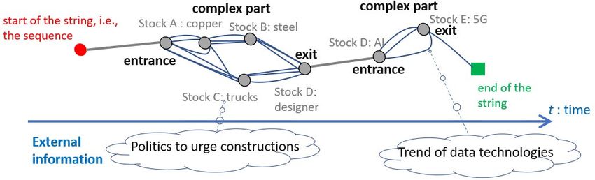
Information 2019, 10, 118                                                                                8 of 21

   real constant)
             end if
     End For
      For each pill
        sent, sext = the first and the last event in pill
        weight(sent) = weight(sext) = ext−ent # assign the pill size as the weight of each event on a wire
     End For

      In this extended TS for sequential basket data, for the newest event si, sj of the same token as si is
searched from the preceding W baskets before si. If such an event as sj is found, all the events between sj
and si and their constituent baskets form a pill. The entrance to the combined pill thus obtained is sj if sj
is the first event revisited in the pill, and si becomes the exit if sj is the last event revisited in the pill.

2.3. Explanation by TS Approach
     It is recommended that the user of the visualized string finds the association between the string
and external information about real events using the following procedure, for explaining the changes
in the sequence. It is assumed that the user is a domain expert, i.e., a stock analyst, with respect to this
study. The string is visualized, not only to obtain the entrances and exits from the pills automatically.
(1) Find nodes (s of “s : t” in Figures 4–6) at entrances or exits, shown in large letters in the string
    compared to the surrounding items, indicating that a larger letter means the entrance to or the
    exit from a larger trend of some set of stocks.
(2) From the string, choose large pills that have a tangled structure as complex parts in Figure 1.
    This is because a large complex pill corresponds to a trend that includes a set of frequent
    events occurring under various subsequences.
(3) Explain the events at the nodes found in (1) above and the complex pills chosen in (2) above,
    correlating closely located events in the string with real events in the external information such
    as the user’s experience, common sense, and news. This part should be a free externalization of
    subjective ideas, rather than adherence to objective facts, in order to collect various
    explanations of possible causalities.
      Such a simple procedure enables easy usage of the string. However, the authors assume that this
human–machine interaction process should be regarded as the essence of TS, and the high
performance of TS stated in Section 3 should be positioned as the evidence to support the user’s belief
in this procedure where TS is employed in positioning entrances and exits of pills in the explanation.

3. Results
      The performance of TS as a tool for change detection is experimentally evaluated here. In Section
3.1, the outline of the weekly data on high-rank price-increasing stocks is shown. Then, the results
presented here are two-fold. In Section 3.2, we show the coincidence of the entrances and exits of the
pills obtained by TS with the beginning of the up-pricing of stocks in the market, by setting W to
several different values. Subsequently, in Section 3.3., we show the coincidence of the entrances and
exits with the major changes in stock prices. Later in Section 4, the qualitative explanation of the
trend shifts, provided by an expert of stock analysis and approved by other analysts, is given for the
output figures of TS.

3.1. Data on Up-Pricing Stocks
     The TS method is applied to the data on stock prices, of which the stocks with the highest price
increase              rate           are             considered              every              week
(http://www.kabu-data.info/neagari/neagari_hizuke_w_1.htm). These data were taken from the
First Section of the Tokyo Stock Market for 592 weeks from 6th July 2007 till 4th January 2019. The
original data included the names of each company but here we consider just the stock ID number of
each firm as shown in Table 1. Each set of top-10 stocks per week are collected as basket data as in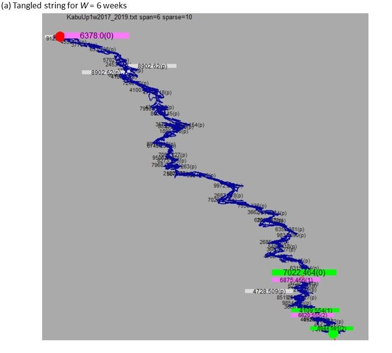
Information 2019, 10, 118                                                                            9 of 21

Table 1, and a similar collection is done for top-5 stocks per week to make a comparison. We also
used data on Japan’s stock price trend (Nikkei Average) for evaluating the performance of TS in
detecting the up/downward price changes in the entire stock market. The data on each stock were
collected as described in Data Availability in the Supplementary Materials section.
     We include experiments for only the top (up-pricing) stocks, and not for the worst
(downpricing) stocks, for three reasons. First, this study aims to enable the detection and the
explanation of changes in a sequence in available data. In comparison with data on the top five or ten
stocks, it is not easy to collect or get approval to use data on the worst stocks. Second, there are firms
in even worse situations than the worst among the listed companies in the stock market—that is,
being at the end of a list does not mean that the situation of the firm is exceptionally bad. The third
and most essential point is that, in this study, the explanation is aimed at changes in the investors’
preferences, i.e., why they preferred positively to buy some stocks rather than act upon negative
motivations to sell stocks (See Section 1).

      Table 1. Weekly data on top up-pricing stocks. The white cells show the data content, where “#n”
      represents the beginning of each basket of top up-pricing stocks for each week, and each 4-digit
      integer shows a stock ID. This table shows a sequence of top-10 up-pricing stocks. A row includes
      five stock IDs for top-5 up-pricing stocks.

                                              No. 1 No. 2   No. 3   …, …, … No. 10
                          6 July 2007    #n   6378 8061     2678    …, …, … 2687
                         13 July 2007    #n   1907 6850     6316    …, …, … 1898
                               …         #n    …     …       …       …, …   …, …
                               …         #n   1907 6378     7999    …, …, … 8934
                        4 January 2019   #n   4992 4344     6465    …, …, … 9501

3.2. TS Visualization with Changing the Window Width W
      The TS visualizations are shown in Figures 4–6. In (a) of each figure, the letters in red and green
show sent and sext, respectively, which are the events that start and end a pill. The letter size shows the
weight, i.e., the number of items in the pill that are started or ended by the event. The node other
than red or green (white node marked by “(p)”) shows the most frequent token in each pill. In each
figure, the curve in (b) shows the average price of all the stocks (Nikkei Average mentioned in Data
Availability). In (b), the larger letters of s in “s:t” in (a) is shown in larger letters at time t. This
procedure can be automatically executed, but has been executed by the authors after discarding
smaller letters such as 4825 that could not be included in (b) due to the space constraint. Note that
each (b) is just for making the discussion in Section 4 understandable and is not the result of the
procedure in Section 2.3. For example, the pill ending at 4825 in Figure 4a was discarded, although
4848 was as small as 4825 in (a). Thus, (b) of Figures 4–6 does not include sent and sext but just
relatively larger letters in (a). However, from the viewpoint of aiding the human explanation of
changes as mentioned in Section 1 with such a figure as Figure 1, the visualization of the letter sizes
together with their connections with the tangled parts is meaningful. For example, a small-sized red
token in (a) should not be ignored if it is larger than other letters nearby on the string and is an
entrance to a small but complex pill. In such a case, the human should link his/her experiences or
common sense to the entrance stock and to stocks in the pills connected to this entrance stock. The
position of nodes and edges in the output of TS are coordinated just for simplifying the string shape
[27], and the structure is not changed.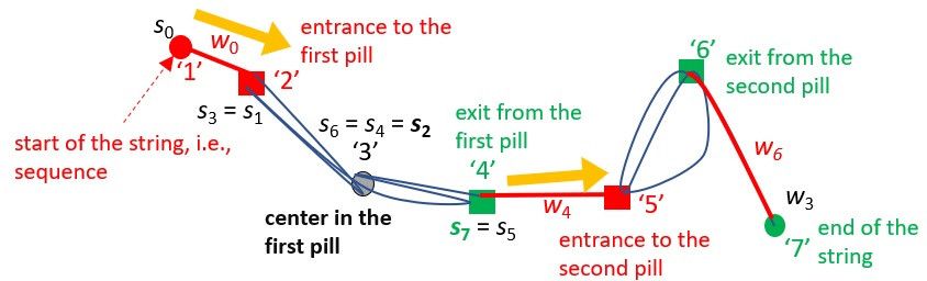
Information 2019, 10, 118 10 of 21
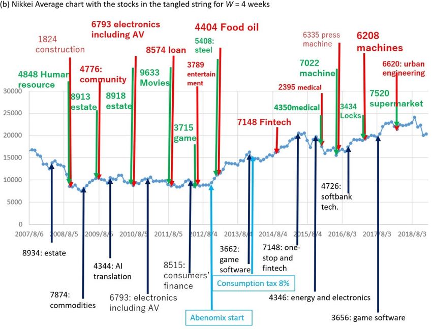
Figure 4. Results of TS for W = 4 (weeks) for the top-10 data. In (a), each red (pill entrance) or green
(pill exit) node show X:Y:Z where X, Y, and Z represent the stock ID, its time (the week counted from
the start of the sequence), and the number of pills counted from the beginning, respectively. The
white node in (a) shows the most frequent token in each pill. (b) shows the timing of the nodes in (a)
on the curve of the average price of all stocks (Nikkei Average).Information 2019, 10, 118 11 of 21
Figure 5. Result of TS for W = 5 (weeks) for the top-10 data. (a,b) mean the same as in Figure 4,
respectively.Information 2019, 10, 118 12 of 21
Figure 6. Result of TS for W = 6 (weeks) for the top-10 data. (a,b) mean the same as in Figure 4,
respectively.
For the top-10 data, in the sequence visualized by TS in Figure 4a, setting window width W to 4
corresponds to the time series of the Nikkei Average in Figure 4b. Because 19 pills were obtained by
TS here for 11 years, setting W to 4 implies investigating the pills for the timescale of approximately
0.58 y, which indicates the minimum required time resolution to distinguish two consecutive pills.Information 2019, 10, 118 13 of 21
For this W value, we do not find an obvious coincidence between the timing of the red/green nodes
and the long-term change points in the stock prices of Nikkei Average in Figure 4b as far as we view
the curve. On the other hand, the results in Figure 5a,b are for setting W to 5. Because we obtained
seven pills for the 11 y, W = 5 means the timescale of ~1.6 y. In this case, we find a substantial
coincidence between the timing of red/green nodes and the long-term changes in the Nikkei
Average. That is, five of six red nodes (except the first of the seven red nodes which turned out to be
the first of the whole sequence, because the distinction between the first node and its previous nodes
is trivial) are within 3 months before the monotonic increase for 6 months or longer in the Nikkei
Average in Figure 5b.
Including the results for other settings of W and the data for the top-5 companies, the precisions
are shown in Table 2. Here precision means the percentage of the red nodes within three months
before the monotonic increase for six months or longer in the Nikkei Average. Note that the number
of entrances and exits become larger for top-5 data than top-10 data if W is set equal. This is because
each pill becomes smaller if the first same token in [t−W, t−1] as the token at time t appears later due
to the lack of information in each basket. All the values in this table are larger than 0.52 (70 weeks
within 3 months before the monotonic increase for 6 months, among all 134 weeks) for a random
choice of alarm. Additionally, coinciding with intuition, the richer data of top-10 comments achieves
higher precision than top-5 as in Table 2.
The stock IDs and the timing of their appearance as entrances or exits of pills are shared in the
Supplementary S1_Data. For a qualitative explanation of the changes considering the red/green
nodes by experts, kindly refer to the next chapter.
Table 2. The precision of the entrances to pills in Nikkei Average.
W=7 W=8 W =9 W = 10
Top 5
0.59 (13/22) 0.67 (8/12) 0.57 (4/7) 0.6 (3/5)
W=3 W=4 W=5 W=6
Top 10
0.55 (21/38) 0.67 (12/18) 0.83 (5/6) 1.0 (2/2)
3.3. Change in Stock Price and the Two Types of Change Points in TS
Next, we evaluated the coincidence of the entrances and the exits from pills to the change, i.e.,
increase and decrease, in stock prices. As in Figure 7, the entrances and the exits are viewed
intuitively to coincide with the starting and halting of the periods of the high-price trend. Figure 7
exemplifies some of the cases where the prices of the stocks increased visually at (from before to
after) the entrance. On the other hand, the price of the stock that started (appeared at the entrance
of) a pill tended to decrease at the time of the exit from the started pill. To evaluate these tendencies,
as in the left half of Table 3, let us compare the trend of the period of length Δt before and after the
entrances of pills, for stocks that appeared as entrances (red letters in TS: see Figure 8a for an
intuitive understanding). The comparison is shown in the right half of Table 3 for stocks that
appeared at exits (green letters in TS, Figure 8b). It can be noted that we did not include cases where
W is less than 3 for top-10 data or less than 7 for top-5 data in Table 3, because the number of pills
came to 50 or more, meaning the average pill lengths were 2.8 months or shorter, i.e., shorter than
any Δt we chose (3 months at least) for this evaluation. In these results, the prices of both change
point stocks, i.e., stocks appearing as entrances and exits, tend to increase after their appearance.
Although the percentage of increase is larger for the top-5 for all Δt, the significance of the increase
(a larger increase than the standard deviation σ) is substantially smaller for top-5 than top-10. Here,
similar to the results in Section 3.2, the results for top-10 data are finer than for top-5 in detecting
high impact changes.
On the other hand, let us investigate the dependence of the precision of the detection of price
increase on the value of W. The probability of price increase of a pill entrance stock is high at (from
Δt before and Δt after) the time that it appeared at the entrance (Figure 9a,d,g,j corresponding to
Figure 8a). These probabilities tend to be higher than a pill-exit stock at the time it appears at the
exit (Figure 9b,e,h,k corresponding to Figure 8b). On the other hand, the probability by which theInformation 2019, 10, 118 14 of 21
price of the stock that appeared at an entrance increased is relatively smaller at the time of the exit
from the pill (as in Figure 9c,f,i,l corresponding to Figure 8c) than the probability at the time it
appeared at the entrance. These tendencies are found especially for larger values of W. This
tendency is interpreted as in the discussions later.
Figure 7. Examples of entrances and exits of pills for top-10 data, located on the time axis of price
changing.Information 2019, 10, 118 15 of 21
Figure 8. Price changes of stocks at pill entrance/pill-exit, at the entrance/exit. (a), (b), and (c) show
the price of an item that appeared at the entrance or the exit that changed as shown in the curve,
respectively. The price was evaluated at the time shown by the dotted vertical line.Information 2019, 10, 118 16 of 21
Figure 9. Price rates (vertical) for entrance/exit items at the entrance/exits. The horizontal axes show
the values of W. See Figure 8 and the main text for the meaning of panel (a–l), and the
Supplementary S2_Data for the real values. For example, (c,f,I,l) show the price-up rates (i.e.,
increase rate in price) of the stock item that appeared at the entrance of a pill, evaluated at the exit of
the same pill, corresponding to Figure 8c, respectively.Information 2019, 10, 118 17 of 21
Table 3. Rates (and the counted numbers in the brackets) of the in/decrease of stock prices at (i.e.,
from the period of length Δt before to Δt after each entrance/exit) the entrances or the exits of pills,
unifying the counts for W = 3, 4, 5, 6 for top-10, W = 7, 8, 9, 10 for top-5. The pair “stock ID: the time”
in a red/green node in Figures 4–6 are counted uniquely (one time for each pair). σ indicates the
standard deviation of the price of each stock for the period of length Δt before t.
Δt 3 mo. 6 mo. 12 mo. 24 mo. 3 mo. 6 mo. 12 mo. 24 mo.
Top-5 Entrances (red) Exits (green)
decrease 0 (0) 0 (0) 0 (0) 0 0.097 (3) 0 0 0
increase 1.0 (43) 1.0 (39) 1.0 (39) 1.0 (34) 0.90 (28) 1.0 (34) 1.0 (34) 1.0 (31)
increase > σ 0.16 (7) 0.18 (7) 0.18 (7) 0.18 (6) 0.097 (3) 0.12 (4) 0.059 (2) 0.16 (5)
Top-10 Entrances (red) Exits (green)
decrease 0.11 (4) 0.19 (7) 0.14 (5) 0.12 (4) 0.15 (6) 0.11 (4) 0.18 (6) 0.09 (3)
increase 0.89 (32) 0.81 (29) 0.85 (29) 0.88 (27) 0.85 (34) 0.89 (34) 0.82 (28) 0.91 (30)
increase > σ 0.75 (27) 0.72 (26) 0.79 (27) 0.71(22) 0.60 (24) 0.69 (26) 0.68 (23) 0.67 (22)
In this paper, we do not compare these results experimentally with methods for prediction
using machine learning as in [4–7], because both the aims of (1) detection of the change points based
on which the future increase/decrease trend can be forecasted in various time scales and (2) to
explain or predict the long-term (e.g., 6 months) trend from a change point both in the entire stock
market and of each stock, by the same visualization method, has not been challenged by an existing
method. Furthermore, the precisions in Table 3 are higher than those associated with the prediction
of up/downpricing by such machine learning techniques (e.g., 65% in [4]), even though changes in
the long-term trend are difficult to predict because of the uncertainty in the long-term future. In the
face of this difficulty, the precision of TS in the worst case to predict a middle/long-term (3 months
or longer) increase in Table 3 is 81% for pill entrance events, 71% for increase larger than the
standard deviation and for richer data, i.e., the top-10 up-pricing stocks. These percentages are
higher than those obtained by existing methods that achieved high accuracy in finding precursors
to drawdowns of the market average [28], or the rate of change oscillators as indicators for
buying/selling [29]. On the other hand, the precision of classification into patterns of decision
opportunities in stock investment exceeds 90% by the machine learning method [7]. Although the
performance criterion differs from ours due to the difference in the goal, we plan toward the future
to borrow this strength so that the explanation of each complex mixture can be made more efficient if
the mixture can be reduced into simple structures or patterns using machine learning.
We also checked the tolerant delay in obtaining a changing point (entrance/exit) by entering a
part of the original data, which do not include the entire target sequence of 11 y, but each tested
sequence, having all the times before the evaluated event and the subsequence of length dt following
the event, is available for various values of dt. This tolerant delay dt means the time we await after the
appearance of a token s, for distinguishing if s is in a pill or on a wire. The tolerant delay in this sense
includes both Δt and δt in the introduction. As a result, for all the pill entrances and exits for W > 3
for top-10 and W > 6 for top-5, we found the same entrances and exits are obtained for dt set to 3
months or larger. This result, however, needs no experimental verification because this is
mathematically supported. That is, we can say that dt is upper-bounded by W−1 for the following
reason. Here, let us count the time using an integer. Suppose the current time t is τ (>0) after the exit
from the last pill (i.e., t−τ). Note there is no pair of same tokens in the time range [t−τ, t] at time t
because this range is not in a pill. When a new token st+1 is added at the next time t+1, it is impossible
to find the same token as st+1 in the time range of [t−τ, t−τ] if τ > W−1, because the time range [t+1−W,
t] is the scope in searching the same token as st+1 and t+1−W is later than t−τ. That is, st−τ cannot be in
the same pill as st+1 as far as τ > W−1, which means that st−τ is on a wire (note: the exit of a pill is on a
wire linked to the next pill) forever if it is on a wire for time length W−1 after its appearance. In
addition, st−τ+1 is on a wire (note: the entrance to a pill is on a wire). Further, it is trivially true that
st−τ+1 is on a pill once it is on a pill. Thus, the tolerant delay is W−1 at the longest. From this principle,Information 2019, 10, 118 18 of 21
under the condition where the span W is set to shorter than 3 months for all the experimental cases,
the tolerant delay is shorter than 3 months.
4. Discussions
Let us discuss the meaning of the results summarized above from the perspective of attaining
the goal of this study, i.e., explanation of changes in various timescales by following the procedure
in Section 2.3. In Figures 4 and 5, an expert stock analyst, who has been a significant figure in
investors’ voting in Japan (listed by Nikkei Veritas) for 16 years (2002 through 2017), found a high
impact change in the period near December 2012 (stock no. 4404 in Figure 4 and no. 4651 in Figure 5,
viewed as large letters as in Section 2.3(1)), corresponds to the political decision by Japan’s Prime
Minister Abe who started to promote the economy for the upward trend through a policy called
Abenomics. Abenomics is a complex mixture of various strategies to activate the Japanese economy,
associated with the substrings viewed to be tangled (as in Section 2.3(2)) between 3789 and 4403 in
Figure 4 and between 4651 and 6333 in Figure 5. The following explanations are given by the same
expert. The stock IDs below were chosen as they were relatively large letters in Section 2.3(1),
tangled substrings in Section 2.3(2), or stocks relevant to them in the market in Section 2.3(3). Three
other experts also agreed with the explanations below, although they had various additional
comments. Although the comments below can be regarded as a consensus of a couple of experts, we
position this section as a discussion about the subjective explanation given by humans regarding
visualized strings rather than objective facts, mainly because it is difficult to collect a sufficiently
large number of experts to obtain statistically significant explanation.
After December 2012, the upward trend was reinforced by investors who preferred to buy the
stocks of stable industries such as healthcare (3660, 4350), energy (4651), and established IT (4229) that
have been generally regarded as low-risk investments, i.e., low volatility [30], because the
governmental bonds fell into distrust due to the lowered interest rate introduced by the Bank of Japan
since April 2013. Although software for smartphones (diverting technologies for games) and urban
development based on big data became trendy according to the frequent tokens in pills in Figures 4–6,
investors lead the market with their preference for low-risk stocks. Here the larger letters (red:
entrances of pills, green: exits) show events of larger weight. The low-volatility stocks did not cause
new long-term trends immediately but contributed to the foundation of innovative industries by the
opening of pills, according to the expert.
In Figure 6, the largest green node 7022 is placed in July 2016 rather than the end of 2012.
Coincidentally, the long-term interest rate came to be increased in Japan [31] from July 2016 and in
the US [32] from August 2016 from the low interest rate since April 2013 above. From the aspect of
stock analysis, this is informative in explaining the general movements in investor interest. That is,
after the inception of Abenomics in 2012, due to the low rate (negative at the beginning of 2016) of
interest introduced by the government of Japan, investors who had been investing in governmental
bonds shifted to buying low-volatility stocks such as specific electric/precision machineries,
healthcare, and medical systems. These low-volatility stocks increased in price since the end of 2012
and priced up further in 2014 and 2016 according to the expert’s comments. Stocks of construction
firms were also bought at a similar interest rate. On the other hand, because of the increase in the
long-term interest rate in Japan and US since the July of 2016, as an effect opposite to the price-up of
low-risk stocks as discussed before for the reduced interest rate due to Abenomics, high-risk stocks
came to be bought relative to low-risk (i.e., low-volatility) stocks. As a result, stocks of new
industries such as digital devices for ultra-highspeed telecommunication, software for smartphones
with the integrated use of big data (on maps and healthcare) and artificial intelligence, and urban
engineering for cities embracing innovative firms such as Shenzhen came to rise recently, such as
stock 6875, which is one of the few entrances of long (W=6) time scale pills in Figure 6.
On the other hand, given below is about the objective results in Table 3 rather than the
human-based explanations above. These results are understandable for a stock appearing at a pill
entrance because the entrance indicates the beginning of the trend that stock is to be bought
frequently. In contrast, the exit stock may be intuitively felt to price down. However, the stock at anInformation 2019, 10, 118 19 of 21
exit means it is of high enough impact enough to break the trend so far, so this tends to be a new
focus of attention of investors. Rather, the tendency of decrease is found at the exit of a pill for the
stock that appeared as the entrance of the same pill. The tendencies found in Figure 9, in summary,
are as follows.
(1) A trend starts at the entrance of a pill and continues during the pill. As a result, the price of the
stock at the entrance of a pill continues to increase during the trend (Figure 9a,d,g,i).
(2) The impact of the stock that appears at the exit fades in a short time because the trend
disappears when the pill disappears. As a result, the price of the stock at the exit of a pill
increases once but decreases sooner than the stock at the entrance (Figure 9b,e,h,k).
(3) A trend ends at the exit of a pill. As a result, the price of the stock at the entrance of a pill
decreases soon after the exit of the same pill (Figure 9c,f,I,l).
(4) The stock tends to increase more for the shorter W because a short W means a reduced capacity
to detect repeating events. Thus, only the entrances/exits of an especially high frequency of
repetition in pills are obtained. However, even for a long W, the price of stocks appearing at
the entrance increases continuously during the period of the trend (all in Figure 9).
Thus, we propose that investors consider positioning all the stocks at the time that they appear
at entrances or at exits, and sell the entrance stock by the time of the pill’s exit or within the delay of
length that is in a negative correlation to the length of the window width W.
5. Conclusions
Here, we extended and applied TS to the data on stocks with increasing value, where various
timescales are mixed corresponding to various investors’ reasons for the buying and/or selling of
stocks. By the use of TS, the connections to/from trends in the market came to be visualized, to aid in
explaining the changes in the market at the desired time scale, associated with middle-term changes
caused by political decisions, and long-term ones due to innovations in the industry. The change
points found as entrances to pills by TS coincide with high precision with the increase in each stock
price. This precision varies by the timescale and the positioning (e.g., at the entrances/exits of pills or
elsewhere) of the stocks in the string presented by TS, and the timing of measuring the increase after
the entrance of a pill. For the time being, the success in selling a stock at the exit of a pill is not as
certain as buying the same stock when it started a pill, according to the probabilities of
up/downpricing that we obtained. In our future work, we plan to assign external knowledge or data
to refine this certainty, as expected in the method M2 in IMDJ.
The strength of TS is also in that the trend shifts in both (1) the overall stock market and (2) the
price of each stock can be explained with one string, whereas (1) and (2) have been analyzed or
discussed separately in the previous work and the literature (e.g., [28,29] above). The direction
taken to enable analysis about the interrelationship between the global dynamics of the market and
the local change in each stock is thus consistent with the fact that the former is composed of the
latter and the latter is affected by the former. Thus, the ability to predict both with a single
visualization fits analysts’ requirement of efficiency. As TS has been created from the requirement
shown in IMDJ, this paper presents evidence that the product of the data market is of practical
utility.
Supplementary Materials: The following are available online at www.mdpi.com/xxx/s1, S1_data (obtained
events): The events obtained as the entrances to or exits from pills as results, with the corresponding dates.
S2_data (up-pricing rates): The price-up rates, showing the rates of cases where the period of length Δt after t
was larger than before t for each event at t that meant the time of (1) the entrance of a pill, (2) the exit of a pill,
and (3) the exit of a pill (but the evaluated price is of the stock that appeared at the entrance).
Author Contributions: Conceptualization of TS: IMDJ, Y.O., and T.H.; Methodology and Software: Y.O.;
Validation: Y.O. and T.Y.
Funding: This work was funded by JST CREST No. JPMJCR1304 and JSPS KAKENHI JP16H01836 and
JP16K12428.Information 2019, 10, 118 20 of 21
Acknowledgments: We appreciate for the stock analysts who provided comments on the results and the
method of TS adopted to stock analysis. We would like to thank Editage for English language editing.
Conflicts of Interest: The authors declare no conflict of interest.
Data Availability: We used data on Japan’s stock price trend chart (Nikkei Average:
https://indexes.nikkei.co.jp/en) for evaluating the performance of TS in detecting the up/downward price
changes in the stock market. Such a scientific use of the data is allowed in
https://indexes.nikkei.co.jp/nkave/archives/file/license_agreement_jp.pdf. The monthly data from 2007 till 2019
are taken, and the average of the max and min prices are taken for each month. The data on each stock has been
collected using http://kabubegin.web.fc2.com/kabu052.html. However, due to the disallowance to copy the data
in the publication, we show only the analysis result below. We also provide the supplementary data below.
References
1. Jagtiani, J.; Lemieux, C. The Roles of Alternative Data and Machine Learning in Fintech Lending: Evidence from
the Lending Club Consumer Platform; WP18-15; Lemieux Federal Reserve Bank of Chicago: Chicago, IL,
USA, 2018; doi:10.21799/frbp.wp.2018.15.
2. Lux, T. The socio-economic dynamics of speculative markets: Interacting agents, chaos, and the fat tails of
return distributions. J. Econ. Behav. Organ. 1998, 33, 143–165, doi:10.1016/S0167-2681(97)00088-7.
3. Lespagnol, V.; Rouchie, J. Trading Volume and Market Efficiency: An Agent Based Model with
Heterogenous Knowledge about Fundamentals. HAL Archives-Ouvertes. 2014. Available online:
https://halshs.archives-ouvertes.fr/halshs-00997573 (accessed on 15 March 2019).
4. Ding, X.; Zhang, Y.; Liu, T.; Duan, J. Deep Learning for Event-Driven Stock Prediction. In Proceedings of
the 24th International Conference on Artificial Intelligence, Buenos Aires, Argentina, 25–31 July 2015; pp.
2327–2333.
5. Dash, R.; Dash, P.K. A hybrid stock trading framework integrating technical analysis with machine
learning techniques. J. Financ. Data Sci. 2016, 2, 42–57, doi:10.1016/j.jfds.2016.03.002.
6. Rajput, V.; Sarika Bobde, S. Stock market forecasting technique literature survey. Int. J. Comput. Sci. Mob.
Comput. 2016, 5, 500–506.
7. Cimino, M.G.C.A.; Bona, F.D.; Foglia, P.; Monaco, M.; Prete, C.A.; Vaglini, G. Stock price forecasting over
adaptive timescale using supervised learning and receptive fields. In Proceedings of the 6th International
Conference on Mining Intelligence and Knowledge Exploration, Cluj-Napoca, Romania, 20–22 December
2018; pp. 279–288, doi:10.1007/978-3-030-05918-7_25.
8. Fama, E.F.; Fisher, L.; Jensen, M.C.; Roll, R. The Adjustment of Stock Prices to New Information. Int. Econ.
Rev. 1969, 10, 1–21, doi:10.2307/2525569.
9. Foster, G. Stock Market Reaction to Estimates of Earnings per Share by Company Officials. J. Account. Res.
1973, 11, 25–27, doi:10.2307/2490279.
10. Yoon, S.; Suge, A.; Takahashi, H. Do news articles have an impact on trading?—Korean market studies
with high frequency data. In New Frontiers in Artificial Intelligence, Proceedings of the JSAI-isAI Workshops,
JURISIN, Tsukuba, Tokyo, 30 June 2018; Springer: Berlin, Germany, 2018; pp. 129–139,
doi:10.1007/978-3-319-93794-6_9.
11. Kaura, M.; Kanga, S. Market Basket Analysis: Identify the changing trends of market data using
association rule mining. Procedia Comput. Sci. 2016, 85, 78–85, doi:10.1016/j.procs.2016.05.180.
12. Ohsawa, Y. Graph-Based Entropy for Detecting Explanatory Signs of Changes in Market. Rev. Socionetwork
Strat. 2018, 12, 183–203, doi:10.1007/s12626-018-0023-8.
13. Iwata, T.; Watanabe, S.; Yamada, T.; Ueda, N. Topic tracking model for analyzing consumer purchase
behavior. In Proceedings of the 21st International Joint Conference on Artificial Intelligence (IJCAI),
Pasadena, CA, USA, 22 July 2009; pp. 1427–1432.
14. Abdulhakim, Q.; Alharbi, B.; Wang, S.; Zhang, X. A PCA-Based Change Detection Framework for
Multidimensional Data Streams: Change Detection in Multidimensional Data Streams. In Proceedings of
the 21th ACM SIGKDD International Conference on Knowledge Discovery and Data Mining, Sydney,
Australia, 10–13 August 2015; pp. 935–944, doi:10.1145/2783258.2783359.
15. Kleinberg, J. Bursty and hierarchical structure in streams. Data Min. Knowl. Discov. 2003, 7, 373–397,
doi:10.1145/775047.775061.
16. Fearnhead, P.; Liu, Z. Online Inference for Multiple Changepoint Problems. J. R. Stat. Soc. Ser. B 2007, 69,
589–605, doi:10.1111/j.1467-9868.2007.00601.x.You can also read