Graph Data Modeling for Political Communication on Twitter
←
→
Page content transcription
If your browser does not render page correctly, please read the page content below
Iowa State University Capstones, Theses and
Graduate Theses and Dissertations
                                                                                                                         Dissertations

2016

Graph Data Modeling for Political Communication
on Twitter
Prashant Kumar
Iowa State University

Follow this and additional works at: https://lib.dr.iastate.edu/etd
     Part of the Computer Sciences Commons

Recommended Citation
Kumar, Prashant, "Graph Data Modeling for Political Communication on Twitter" (2016). Graduate Theses and Dissertations. 15949.
https://lib.dr.iastate.edu/etd/15949

This Thesis is brought to you for free and open access by the Iowa State University Capstones, Theses and Dissertations at Iowa State University Digital
Repository. It has been accepted for inclusion in Graduate Theses and Dissertations by an authorized administrator of Iowa State University Digital
Repository. For more information, please contact digirep@iastate.edu.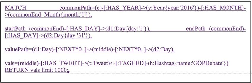
Graph data modeling for political communication on Twitter

                               by

                       Prashant Kumar

        A thesis submitted to the graduate faculty
 in partial fulfillment of the requirements for the degree of
                 MASTER OF SCIENCE

                 Major: Computer Science

               Program of Study Committee:
         Wallapak Tavanapong, Major Professor
                      Johnny S. Wong
                         Jan Boyles

                   Iowa State University
                        Ames, Iowa
                            2016

 Copyright © Prashant Kumar, 2016. All rights reserved.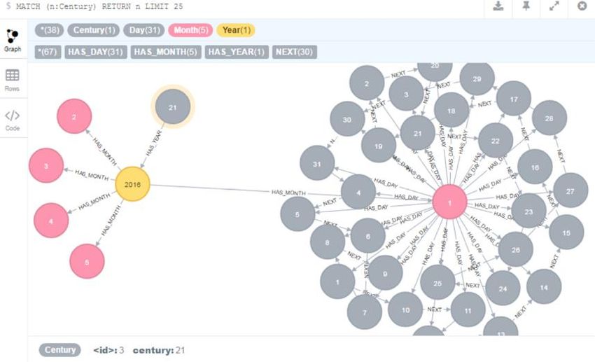
ii

                                        DEDICATION
       I lovingly dedicate this thesis to my mother, Maya. Her support and love has
sustained me throughout this journey. I also dedicate this work to my father, Bijendra
Singh and sister, Preeti. I will always appreciate all they have done.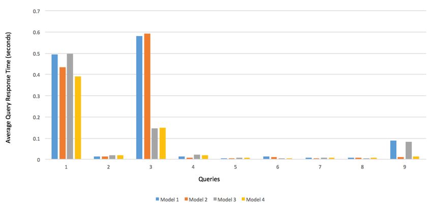
iii
                                                  TABLE OF CONTENTS
                                                                                                                         Page
LIST OF TABLE ........................................................................................................iv
LIST OF FIGURES ....................................................................................................v
ACKNOWLEDGEMENTS .......................................................................................vi
ABSTRACT .................................................................................................................vii
CHAPTER 1 INTRODUCTION ...............................................................................1
   1.1 Contributions.......................................................................................................2
   1.2 Organization ........................................................................................................3
CHAPTER 2 RELATED WORK..............................................................................4
   2.1 Query Optimization and Indexing Mechanism in Neo4j ....................................4
  2.2 Guidelines for Graph Data Model Design ...........................................................6
  2.3 Query Optimization via Graph Structure Change ................................................7
CHAPTER 3 PROPOSED GRAPH DATA MODELING FOR POLITICAL
                     COMMUNICATION ON TWITTER ..............................................12
   3.1 Questions of Interest to Political Communication ..............................................12
   3.2 Data collection and storage techniques used ......................................................18
   3.3 Graph Data Modeling .........................................................................................19
CHAPTER 4 EXPERIMENTAL RESULT AND PERFORMANCE
                     EVALUATION ...................................................................................25
   4.1 Data Collection and Database Creation ..............................................................25
   4.2 Performance Metric and Measurements .............................................................26
   4.3 Experimental Results ..........................................................................................27
   4.4 Important Findings ..............................................................................................30
   4.5 Limitations of the Experiment ............................................................................31
   4.6 Findings about Political Communication............................................................32
CHAPTER 5 CONCLUSION AND FUTURE WORK ..........................................33
BIBLIOGRAPHY .......................................................................................................34
APPENDIX A. CYPHER QUERIES ........................................................................38
APPENDIX B. THE STEPS TO RUN THE PROGRAM ARE AS FOLLOWS ..46
iv
LIST OF TABLES
Page
Table 3.1 Queries of Interest to Communication Scholars ........................................13
Table 3.2 Summary of the design choice to study query performance ......................19
Table 4.1 Collected Data............................................................................................25
Table 4.2 Sizes of Data Models .................................................................................26
Table 4.3.1 Average time taken by queries in seconds .................................................27v
LIST OF FIGURES
Page
Figure 2.1 Cypher query execution process .................................................................4
Figure 2.2 Time tree example ......................................................................................8
Figure 2.3 Cypher Query Execution ............................................................................8
Figure 2.4 Cypher query utilizing the time tree ...........................................................9
Figure 3.1 Data Model 1 ..............................................................................................20
Figure 3.2 Data Model 2 ..............................................................................................22
Figure 3.3 Data Model 3 ..............................................................................................23
Figure 3.4 Data Model 4 ..............................................................................................24
Figure 4.1 Process for importing tweets and related data ............................................25
Figure 4.2.1 Comparison chart for Q1-Q9 ...................................................................28
Figure 4.2.2 Comparison chart for Q10-Q17 ...............................................................29
Figure 4.2.3 Comparison chart for Q18-Q25 ...............................................................30vi
ACKNOWLEDGEMENTS
I would first like to thank my thesis advisor professor, Dr. Wallapak Tavanapong for
her continuous support, enthusiasm, encouragement, motivation, insightful comments and
providing me with the right direction whenever she thought I needed for research and writing
this thesis. I value her patience she has shown with me and her passionate participation and
input during our association.
My sincere thanks to my POS committee member Dr. Jan Lauren Boyles for her
collaboration and providing me with the opportunity to learn about the latest developments
in the field of political communication and social media analysis. Her feedback has been
essential and laid a solid foundation for my work.
A big thanks to my co-major professor Dr. Johnny Wong for his time and hard Q&A
sessions. I also want to thank him and Dr. Tavanapong for all the good food and fun we had
in this association. In addition, I would like to thank Dr. Samik Basu for keeping his door
always open to listen and provide suggestions whenever I needed.
Special thanks to my friends for being there for me and supporting me throughout
this entire journey.vii
ABSTRACT
Twitter has become a political reality where political parties, presidential candidates,
legislatures and journalists post tweets about the latest events sharing texts, pictures,
hashtags, URLs, and mentioning other users. Gaining insight from the vast amount of
political data on Twitter is only possible with proper computational tools.
We propose to store and manage Twitter data in an optimized Neo4j graph database
for serving queries about political communication among state legislators of 50 U.S. states,
state reporters, and presidential candidates for the 2016 presidential election. Our rationale
for selecting this relatively new database technology is threefold: (1) ease of use in explicitly
modeling and visualizing communication relationships among entities of interest; (2)
flexibility to evolve the database overtime to quickly adapt to changes in user requirements;
and (3) user-friendly intuitive query interface. We developed a Python-based Google App
Engine application using Twitter API to collect tweets from the Twitter’s handlers of the
aforementioned political actors. We employed best practice guidelines in graph database
design to develop five different database models in order to distinguish the impact of each
query optimization technique. We evaluated each of the models on the same set of tweets
posted during January 1, 2016 to November 11, 2016 using the same set of queries of interest
to political communication scholars in terms of the average query response times. Our
experimental results confirmed the benefits of the best practice design guidelines. In addition,
they show that the optimized database model is able to provide significant improvement in
query response times. Reducing the number of hops used in the graph queries and using
database indexes on most commonly used attributes reduced the average query response time
in our dataset by as much as 74.52% and by 85.27%, respectively, compared to the reference
model. Nevertheless, the reduction in the average query response time comes with the cost
of the increase in graph database relationship store size by 5.49% compared to the reference
model.
Our contributions are as follows. (1) The optimized Neo4j graph database that will
be updated weekly with new tweets; the access to this database can be made available to
political communication scholars. (2) The above findings added to currently limitedviii guidelines in graph database designs. (3) The findings about political communication prior to the Iowa caucus of the 2016 primary presidential election.
1

                              CHAPTER 1. INTRODUCTION
       Due to ever expanding data on the web at a very fast rate and the rise of online
journalism [1, 2], there is a need for effective and efficient ways of processing abundant data
and presenting relevant and important information [3]. Twitter, a popular micro-blogging
platform [4], is a vast source of data including political data that have gained tremendous
interests among social science research studies [5, 6, 7]. Jungherr surveyed 115 articles about
the use of Twitter in politics [7]. The survey mentions the usage of Twitter by politicians, by
constituents during elections, and by campaign strategists to facilitate campaign events.
Twitter has become an important tool for data journalists for political news [8-12].
       To the best of our knowledge, the communications on Twitter among this group of
political actors, namely, state legislators, state reporters, and presidential candidates have not
been studied because of lack of proper computational tools. Some interesting questions are
as follows. In a given time period, who are influential among state legislators or reporters?
What hashtags or URLs are popular among this group and whether they imply or carry any
agendas? Do state reporters’ tweets carry the same message as those in state legislators’
tweets? Is there a group of state legislators who frequently mention each other or retweet
each other’s tweets? Are they in the same state or across states? Is there a similar interaction
among a group of state reporters?
       This thesis focuses on designing an optimized database for serving the first set of
queries about political communication on Twitter within the above group of political actors.
We propose to use a Neo4j graph database management system to manage the database due
to the following reasons. (1) At the time of this writing, Neo4j is the most widely used graph
database management system (GDBMS) [13]. It has good documentation and is able to
integrate with several third-party programs such as Tableau [14], a popularly used
visualization tool by data journalists. (2) Neo4j supports a simple property graph model that
explicitly models relationships as edges among entities (modeled as nodes) of interest;
therefore, we can model communication relationships among political actors explicitly. (3)
Neo4j query language is called Cypher which is declarative yet powerful to let users
formulate their text queries into Cypher queries relatively easy. (4) GDBMS does not have a
schema; hence, it can evolve quickly in order to adapt to rapid changes in user requirements
[15, 16]. (5) Neo4j, in particular, has a user-friendly query interface that supports
2
visualization of query results in a graphical format. Last, in terms of query response time,
Neo4j was shown to offer better query performance compared to other GDBMS such as DEX
[17], NativeSail [18] and HypergraphDB [19].
GDBMS is relatively new database management technology. Compared to an
established database management systems such as relational database management systems
(RDBMS) [20] or other No-SQL database management systems [21], GDBMS is more
intuitive for modeling, querying, and visualizing complex relationship data [22, 23]. Nodes
and edges are the key elements of any graph data model. There are several graph data models
such as a simple property graph model [24], a Resource Description Framework graph model
[25], and a hypergraph model [26]. In a simple property graph model, a single node
represents one real-world entity of interest, e.g. a person, a category, a place or a thing. An
edge represents an individual relationship between two nodes in the graph. Properties of
entities or relationships are modeled as properties of individual nodes or individual edges,
respectively. Nodes can be grouped into the same group and assigned the same label name.
A similar grouping of edges is also done. GDBMS supports Create, Read, Update and Delete
(CRUD) operations [27, 28] of nodes and edges. The network of nodes and connected edges
is what we term the structure of the graph in this thesis. The graph structure can significantly
influence query response times for the same returned results as shown in previous studies of
graph databases about movies [29] and about tweets and Twitter users [30, 31]. Indexing
frameworks together with rule and cost based optimizations for graph queries have been
developed [32-35].
1.1 Contributions
In this thesis work, we designed a set of queries about political communication on
Twitter among presidential candidates, state reporters, house representatives, senates and
senators. We developed a Python-based Google App Engine application using Twitter API
to collect tweets from the Twitter’s handlers of the aforementioned political actors. We
collected 167,671 tweets during January 1, 2016 to November 11, 2016. We designed five
different graph data models and determined the most efficient data model for our set of
queries written in Neo4j’s query language called Cypher [36]. Our experimental results show
that the key to achieve low query response time is (1) to use fewer numbers of hops between3
nodes in the queries and (2) to query using schema indexing on attributes that are most
frequently used in the query conditions. The largest improvements were of 74.52% and
85.27% in average query response time compared to those of the reference model due to
these two key features, respectively.
Our contributions are the following. (1) The optimized Neo4j graph database that will
be updated weekly with new tweets; the access to this database can be made available to
political communication scholars who would use the pre-defined Cypher queries to obtain
the information or use Tableau to visualize the query results from our database. (2) The
findings on graph query optimization to be added to the currently limited guidelines in graph
database designs. (3) The findings about political communication prior to the Iowa caucus
of the 2016 primary presidential election that the database queries reveal.
1.2 Organization
In Chapter 2, we discuss related work on graph databases with emphasis on
techniques for improving performance of graph database queries. Chapter 3 presents the
proposed graph data models. In Chapter 4, we present experimental results and findings on
how to design an efficient graph data model, when we should create a new node for an entity,
when to introduce new edges in our data model, and when and how to use indexing to
maximize the performance of the Neo4j Cypher queries and other considerations to keep in
mind while designing the Cypher queries in order for them to offer low query response time.4
CHAPTER 2. RELATED WORK
In this chapter, we present related work relevant to techniques for improving
performance of graph database queries. In Section 2.1, we provide background on indexing
features and internal query optimization in Neo4j [37]. In Section 2.2, the graph design
guidelines given by Neo4j [38] were summarized. In Section 2.3, we describe query
optimization techniques by adding additional edges and/or nodes to direct the search to only
relevant nodes such as the “time-tree” approach [39] that was proposed to support time-based
range queries to find events occurring in a given time period.
2.1 Query Optimization and Indexing Mechanism in Neo4j
Indexing is an internal data structure of a database management system for narrowing
down the search space for the data of interest. Neo4j provides two indexing mechanisms:
label indexing and schema indexing [40]. Label indexing is automatically created when a
label is created. However, schema indexes have to be manually created given a label name
and one attribute name of the label to create an index on. For instance, a user can manually
create an index on the “name” attribute of the “User” label. Unlike RDBMS, a composite
search key of several attributes is not allowed. Schema indexing is automatically considered
in the following cases. (1) When there exists an equality comparison of the indexed attribute
and a value without any function performed on the attribute. (2) When the indexed attribute
is used in the “in” clause. (3) When the use of the index is explicitly specified in the query.
The schema indexing is not considered when the indexed attribute appears in the inexact
matching condition or when a function is applied on the indexed attribute even in equality
condition.
Figure 2.1 Cypher query execution process5
Neo4j executes a Cypher query in a sequence of steps as shown in Figure 2.1. It first
parses the input query and tokenizes it to build the corresponding abstract syntax tree (AST
in Figure 2.1). It does basic syntax error checking of the query. If the query has no syntax
error, Neo4j continues with semantic analysis. Neo4j’s documentation does not provide
concrete details about how semantic analysis is done. We speculate that this process is similar
to a typical semantic analysis process in RDBMS, which includes checking for undefined
attributes, for incompatible operand types with the operation in the query, and for incorrect
semantic of the query graph such as missing the join condition [41]. Next, Neo4j normalizes
and optimizes the abstract syntax tree. Then, it rewrites the query such that all the labels and
types are moved from the match clause in the query to the where clause and converts all
equality statements (e.g., hashtag=“GOPDebate”) into an “In” statement (e.g., hashtag in
[“GopDebate”]). One or more logical query plans are then created, depending on which
query planner is used. A query plan/tree is a tree of operators such as NodeByLabelScan,
NodeUniqueIndexSeek, CartesianProduct, ShortestPath, and Limit. Each operator takes no
more than two operands (inputs). Once the final logical plan is selected, the algorithm for
each logical operator in the final logical query plan is determined, which results in the
physical query plan.
The early version of Neo4j only supports a rule-based planner. Although it utilizes
relevant indexes to produce query plans [42], no query cost is estimated and no statistics are
used in the rule-based planner. Starting from version 2.2.0, Neo4j offers a cost-based planner
in addition to the rule-based planner. Utilizing the same principles in RDBMS, Neo4j cost-
based planner estimates the cost of each logical query plan using statistics kept in the
database such as label and index selectivity factors of the labels or indexes used in the query.
Selectivity factor is the ratio of the number of output rows produced by an operator to the
number of input rows coming in to the operator. The query tree with high selectivity (i.e.,
low selectivity factor) at the base of the query tree tends to give a faster query execution time
because less results are available to subsequent operators in the tree to process. Several
logical query plans are considered by Neo4j cost-based planner. The cheapest plan is then
selected for execution by a greedy algorithm in Neo4j version 2.2 or a dynamic programming
algorithm in Neo4j version 2.3. Because the cost-based planner offers much better
performance than the rule based planner, all read-only Cypher queries use the cost-based6
planner by default. To force the use of the rule-based planner, either set the
dbms.Cypher.planner option to RULE in the configuration file, which forces the rule-
based planner on all Cypher queries submitted to this Neo4j server, or prepend CYPHER
planner = rule before the Cypher query, which forces the use of the rule-based planner only
this query.
2.2 Guidelines for Graph Data Model Design
Since GDBMS is relatively new technology, there are very few principles available
for designing graph databases. Neo4j’s developers provide some guidelines for graph
database model design [43]. Real-world entities are typically modeled as nodes and nodes
with similar properties are grouped into a label. Simple properties (single-value properties)
should be kept as node properties. A composite property consisting of multiple components,
for instance, an address consisting of the first line, the second line, city, state, and zip code,
should be broken down into multiple nodes, one for each component of the property. These
nodes are linked via labeled edges with the main node.
Two-way relationships among entities are modeled as edges. Quality of relationships
is modeled as the property of the edge. If the relationship involves more than two entities, an
intermediate node is used to link all the node entities. The data model should attempt to
reduce redundant data in the database to reduce the search space. Nodes can be linked in a
linear fashion to indicate the order they occur in time. Nodes can be linked in a tree fashion
termed multi-level indexing structure where the root node has its children nodes representing
individual years; each year node has its children nodes representing individual months; each
month node has its children nodes representing individual days; the children nodes are linked
together in chronological order. Each day node has its children representing individual events
on that day. This idea is similar to the time-tree idea mentioned in the next section. If we
only keep the date of the events as the property in the event node and use it in the query to
find events in a particular time period, Neo4j needs to search through all the event nodes to
find the event nodes in the required time period. We can use the multi-level indexing
structure to find the beginning node representing the start date and the end node representing
the end date in the given time interval and only search through the nodes linked in between
these two nodes. One may ask why not using schema indexing on the event date property7
instead of creating the additional multi-level indexing structure, which further increases the
size of the database. The reason is that Neo4j will not use schema indexing if a function is
applied on an attribute value in which the index exists. A date consists of day, month, and
year. If we want to look at a particular date, a function has to be applied to extract the date,
which prohibits Neo4j from using the indexing on this property.
2.3 Query Optimization via Graph Structure Change
We describe the application of the time-tree approach using our dataset. To model
each tweet and its various properties such as time when it was posted and the tweet text, we
can use a node with the label “Tweet” to store properties of each tweet as node properties.
We refer to the nodes having this label as Tweet nodes. One naïve approach for retrieving
tweets posted within a given time range is to compare it with the corresponding property
value of Tweet nodes, but it can be very time consuming since Neo4j has to check this
property value against those of all the Tweet nodes in the database, depending on the number
of tweet nodes in the database. Furthermore, showing tweets posted in a particular order by
time requires further sorting of the results, which increases the query processing overhead.
Therefore, multi-level tree data structures were introduced to support queries for data in a
given time range [44]. Tweet nodes are attached to the leaves of the time tree. To show tweets
posted within a specified time period is to traverse through relevant branches in the time tree
structure. In Figure 2.2, the time tree has a root node labelled as a “Century” node, followed
by nodes representing individual years on the first level, nodes representing individual
months on the second level, nodes representing individual days on the third level, and so on
[45]. The individual leaf nodes of the time tree has edges to tweet nodes posted at that time
as illustrated in Figure 2.2.8
Figure 2.2 Time tree example
Figure 2.3 “Tweet” nodes attached to “Day” nodes linked via “:NEXT” edges9
In order to get tweets posted in a given time period using the time tree, we rewrite
the query to find the starting path node and ending path node and collect the tweets attached
to the day nodes which are ordered and connected through the next relationship edge in
Neo4j. See the rewritten query in Figure 2.4 for tweets with the hashtag “GOPDebate” in it
during January 2016.
Figure 2.4 Cypher query utilizing the time tree
There are two approaches for creating the time tree. The first approach is to create
the tree with nodes and labels representing the predefined number of years (e.g., Year nodes),
months (e.g., Month nodes), and days (e.g., Day nodes), respectively. Then, attach each
Tweet node to the Day node the tweet was posted. But the problem with this approach is that
we should know in advance about the time range of the tweets to add to the database. The
second approach is to create the time tree nodes dynamically while adding the tweets to the
database [41]. The time tree can further be expanded to include the time information about
the tweets posted.
Cattuto et al. introduced a graph data model for representing and efficiently querying
the time-varying social network data in Neo4j [31]. They collected data from participants
wearing badges equipped with active Radio Frequency Identification devices during the 20th
ACM Hypertext 2009 conference from June 29th to July 1st 2009. Their model allows rich
queries involving combinations of a social network topology. Their proposed data model
included a similar time-tree graph structure to support time-based range queries. The model
was implemented in Neo4j and was shown to perform well.
Goonetilleke et al. stored micro-blogging queries in most widely used graph
databases: Neo4j and Sparksee [30]. The data model is simple, consisting of user nodes,10
tweet nodes, and hashtag nodes with posts, mentions, follows, and retweets relationships
among user nodes and tags between tweet nodes and hashtag nodes. No time-tree like
structure was used to support range search queries in a given time period. The authors
implemented their graph in Neo4j with nearly 50 million nodes and 326 million edges. They
used Twitter as the data source having 284 million follows relationships among 24 million
users. Their simple queries included select queries, adjacency queries to retrieve the
immediate neighborhood of a node. For advanced queries, they used the count, order by, and
limit clauses in Neo4j. Other queries included co-occurrence queries, recommendation and
influence queries. In their work, they did not evaluate the performance of the graph database
management systems.
2.3 Other GDBMS Query Optimization, Indexing, and Benchmarking
Dai et al. investigated the performance of rule-based query optimization by sharing the state
and computation between multiple queries [32]. They have introduced new abstractions,
physical operators, and rules. The experiment results were measured on both real world
datasets and synthetic benchmark. However, their framework is limited to a specific set of
queries. They have not tested their framework against a cost-based optimizer which is the
default planner for the latest version of Neo4j as it performs much better than rule-based
planners. Trißl proposed a cost-based optimization framework for graph queries where graph
nodes and edges are stored in RDBMS [35]. In this work, two implementations of path
operators were introduced. The performance of the proposed method was evaluated on
synthetic data only. More work is needed for the framework to handle path length and path
queries.
Zhao and Han proposed a new pattern-based graph indexing framework using a
decomposed shortest path algorithm for efficiently searching graph structures in large
networks [33]. They implemented their framework for searching protein structures in a
biological graph database. They evaluated the performance of their framework on both
synthetic and real biological datasets. However, they still need to develop their framework
for large graph networks that grow over time and also need to address the issue of noise and
failure in the network before their indexing technique can be adopted. Williams et al.
proposed a novel method of indexing the graph databases for subgraph isomorphism queries11
and similarity queries [46]. They tested the performance of their method on protein motif
datasets and on synthetic datasets as well. However, their technique is limited to small graphs
(less than ~ 20 nodes).
Benchmarking of GDBMS was also intensively studied as summarized in Tang’s
thesis [47]. Ciglan et al. discussed various challenges of developing fair benchmarking
methodologies of graph traversal operations [18]. They implemented their benchmarking
suite for 5 graph databases: Neo4j, DEX, OrientDB, NativeSail and SGDB. They performed
experiments with the datasets having nodes varying from 1,000 to 100,000 vertices. The
larger datasets had vertices varying from 200, 400, 800 thousands and 1 million vertices.
They developed their design to test the ability of GDBMS in different memory constrained
environments performing breath first traversal and community detection. For the
benchmarking dataset, they used LFR-Benchmark generator which was primarily designed
for testing algorithms for community detection in a graph. They concluded that operations
involving local traversals in a large network are more suitable for the tested systems than
operations involving traversals of the whole graph structure. Dominguez-Sal et al. evaluated
the performance of four graph databases: Neo4j, Jena, Hypergraph DB and DEX. Using their
HPC Graph Analysis Benchmark, they tested the performance on different graph sizes. They
showed that Neo4j and DEX are the most efficient ones.
For the cloud environments, Dayarathna and Suzumura developed XGDBench
benchmarking framework [48]. They used Multiplicative Attribute Graph (MAG) model for
realistic modeling of attributes of the graph databases and used the R-MAT algorithm to
build the graphs for different sizes and edge densities. They evaluated the applicability of the
MAG model and conducted performance evaluation. For small graphs, all GDBMS
performed reasonably, but only Neo4j and DEX could load the largest datasets. DEX scales
better traversing 15K traversing edges per second but Neo4j had a better throughput for some
operations. DEX had best performance for most operations, and in operations in which Neo4j
was the fastest, DEX performance was comparable to that of Neo4j.12
CHAPTER 3
PROPOSED GRAPH DATA MODELLING FOR POLITICAL COMMUNICATION
ON TWITTER
In this chapter, we present our proposed approach. We start with questions about
political communication in Section 3.1. In Section 3.2, we present the process for collecting
tweets from Twitter and the challenges we faced. In Section 3.3, we discuss our design of
five different graph data models along with the rationale. We provide Cypher queries for
each data model in the Appendix A. Appendix B provides description on how to run the data
collection program.
3.1 Questions of Interest to Political Communication
Communication scholars are interested in studying communication on Twitter to
produce some meaningful stories such as important political communication on Twitter
between US state reporters and political leaders and the impact on political policy making.
Under a consultation with a communication scholar, we design 26 queries of her interest as
listed in Table 3.1. Hashtags are assumed to carry out common interests. Therefore, hashtags
used in tweets, users’ mentions in tweets, and retweets among different parties are of
particular interests. Each user has an associated category among presidential candidate,
house representative, reporter, senator, senate, and house. Each user also has an associated
political party to which she belongs. A screen name of a user is used to represent a user’s
name as all the users must have their screen name but may leave their name empty.13
Table 3.1 Queries of Interest to Communication Scholars
Q1 Find top k most retweeted tweets by users in GOP and Democrat parties in a given
month; show the retweet count, tweet text, user’s name, and user’s party in
descending order of the retweet count.
Example parameter values: k is 100 and the month is Jan. 2016
Rationale: This query finds k most influential tweets in a given month and the
user who posted them.
Q2 In a given month, find top k users who used a given hashtag in a tweet with the
most number of retweets; show user’s name, user’s party, tweet text, and retweet
count in descending order of the retweet count.
Example parameter values: k is 100; hashtag is GOPDebate and the month is
Jan. 2016.
Rationale: This query finds top k influential users who used a given hashtag that
may represent a certain agenda.
Q3 Find top k hashtags that appeared in the most number of states; show the number
of states it appeared in, the list of the distinct states it appeared, and the hashtag
in descending order of the number of distinct states the hashtag appeared.
Example parameter values: k is 100
Rationale: This query finds top k hashtags that are most widely spread across
states, which could indicate a certain agenda that is widely discussed.
Q4 Find distinct states along with the month and the date of a tweet posted by state
legislature (senate, senators, house, and house representatives) or state reporters
using a given hashtag in a given year.
Example parameter values: hashtag is GOPDebate; the year is 2016.
Rationale: This query aims to find the spread across states of a given hashtag
among state legislatures and reporters that could represents a topic of interest
along with the timeline of the discussion.14
Table 3.1 (continued)
Q5 Find tweets that have a given hashtag posted by users of a given state for a given
month. Show tweet text and retweet count in descending order of the retweet
count.
Example parameter values: hashtag is GOPDebate; the state is New Jersey; the
month is Jan. 2016.
Rationale: This query finds most influential users in a given state for a particular
topic of interest (hashtag).
Q6 Find k users who used a given set of hashtags in their tweets. Show the user’s
name and the US state to which the user belongs in the alphabetical order of the
names.
Example parameter values: hashtags are GOPDebate, DemDebate, GOP; k is
100.
Rationale: This query finds k users who share similar interests (based on
hashtags).
Q7 Find users who used a given hashtag in a given state in a given month; show the
count of tweets posted with that hashtag along with the user’s name and category
in descending order of the tweet counts.
Example parameter values: hashtag is GOPDebate and the state is New Jersey;
month is Jan. 2016.
Rationale: This query finds users who used a given hashtag most often in a given
state. These users could influence an agenda within the state.
Q8 Find k tweets posted by a given user for a given hashtag in a given state for a given
month. Show the tweet text and the user’s name.
Example parameter values: k is 1000; the user’s name is SusanKLivo; the
hashtag is GOPDebate; the state is New Jersey; the month is Jan. 2016.
Rationale: This query is to be used after Q7 to find out more about the content of
the tweets with the hashtag of interest.15
Table 3.1 (continued)
Q9 Find top k most followed users; show the user’s name, the user’s party, and the
number of followers in descending order of the number of followers.
Example parameter values: category values are GOP or democrat.
Rationale: This query finds the most influential user measured by the number of
followers; this query can be extended to find the influential user of a certain
category or a certain party.
Q10 Find the list of distinct hashtags that appeared in one of the states in a given list in
a given month; show the list of the hashtags and the state in which they appeared.
Example parameter values: state list includes Ohio, Alaska, Alabama; the month
is Jan. 2016.
Rationale: This query is to find common interest among the user in the states of
interest.
Q11 Find tweets with hashtags posted by republican (GOP) or democrat members of a
given state in a given month; show the tweet text, the hashtag, the user’s name of
the user who posted the tweet, and the user’s party.
Example parameter values: state is Ohio; the month is Jan. 2016
Rationale: This query allows exploration of the context in which the hashtags
were used.
Q12 Show hashtags, tweets, user, state nodes for a given state for a given month with
the maximum limit of k results
Example parameter values: state is Ohio; the month is Jan. 2016; k is 1000.
Rationale: This query gives detailed activities in a given state.
Q13 Show at most k nodes representing tweets that has a given hashtag used in a given
month.
Example parameter values: hashtag is GOPDebate; the month is Jan. 2016; k is
100.16
Table 3.1 (continued)
Q14 Find at most k users who used a given hashtag in their tweet in a given month;
show user’s name, user’s party, and the name of the state the user belong in
increasing order of the tweet posted date.
Example parameter values: hashtag is GOPDebate; the month is Jan. 2016; k is
1000.
Rationale: This query finds users who used the given hashtag in the given period
of time.
Q15 Show user’s name and user’s state along with the list of URLs used in tweets
posted by these user for a given month in ascending order of the dates the tweets
were posted.
Example parameter values: user’s party is GOP for Mar. 2016
Rationale: This query finds the URLs shared by user of a given party.
Q16 Find top k tweets of users who belong to one of the parties in the given list of
parties and in a given month. Show user’s name, user’s party, tweet text, retweet
count, and the url used in the tweet in descending order of the retweet count
Example parameter values: user’s party is GOP or democrat for the month of
Jan. 2016; k=100.
Rationale: This query finds the most influential tweets along with the user who
posted them and the urls used by the user.
Q17 Find k users of a given party in a given month. Show user’s name, user’s party,
and the list of URLs used by the user in their tweets.
Parameter values: user’s party is GOP for the month of Jan. 2016; k=100.
Rationale: This query helps us to find the URLs shared by members of the same
political party.
Q18 Find k users who were mentioned in tweets of users of a given party; show tweet
text, user’s name, user’s state, and name of the user mentioned in the tweet in
ascending order of the days of the month.
Parameter values: user’s party is GOP for the month of Jan. 2016; k=1000;
Rationale: This query finds interactions among users on Twitter.17
Table 3.1 (continued)
Q19 Find k users of a given party and users who they mentioned in their tweets in a
given month.
Parameter values: user’s party is GOP; the month is Jan. 2016; k=1000
Rationale: This query finds interactions among users on Twitter.
Q20 Find k hashtags used by users of a given state in a given month; Show hashtag
nodes, day nodes, month node, and year node.
Parameter values: state is New Jersey for the month of Jan. 2016; k=1000.
Rationale: This query visualizes these hashtags and connections.
Q21 Find top k hashtags among users of a given party in a given month; show the
hashtags and count of the number of time the hashtag appeared in descending
order of the count.
Example parameter values: user’s party is GOP; the month is Jan. 2016;
k=1000.
Rationale: This query finds k most popular hashtags.
Q22 Find top k hashtags among all the users; show the number of tweets (count) that
each hashtag has been used and the list of distinct user’s states of these tweets,
and the count of the distinct states, in descending order of the tweet count.
Example parameter values: Month is Jan. 2016; k=1000
Rationale: This query finds the spread of popular hashtags among state.
Q23 Find top k hashtags posted by users in a given list of parties in a given list of
months in a range of days. Show the hashtag and the count of the tweets the
hashtag appeared in the descending order of the count
Example parameter values: party list contains GOP and democrat; the month is
Jan. 2016 and Feb. 2016 and the day range is 1-8.
Rationale: This query finds popular hashtags during certain days (e.g., before
Iowa caucus).18
Table 3.1 (continued)
Q24 Find top k hashtags posted by users in a given list of parties in a given month;
show the hashtag, the count of tweets the hashtag appeared in.
Example parameter values: user’s party list contains GOP and democrat; the
month is Jan. 2016; k=1000.
Rationale: This query finds the most popular hashtags posted by users in a given
list of parties.
Q25 Find k users mentioned in tweets by users in a given party list in a given month;
show tweet text, user’s name and the name of the user mentioned in ascending
order of the month and the day of the tweet.
Example parameter values: user’s party list consists of GOP and democrat; the
list of month is Jan. 2016 and Feb. 2016; k=10,000.
Rationale: This query helps us to find the users mentioned.
3.2 Data collection and storage techniques used
For our data collection we focused on Twitter accounts of US state reporters,
Presidential Candidates, House Representatives, Senate and Senators. Overall, we collected
tweets posted by Twitter accounts.
In order to collect tweets from Twitter, we developed an application using Python
2.7.10 communicating with Neo4j 2.3.3 which is the most commonly deployed graph
database worldwide. Py2neo 2.0.9 and Tweepy 2.2 python libraries were used in your
application. Py2neo is a library to interact with Neo4j whereas Tweepy is a library for
interacting with the Twitter Search API, which is a part of Twitter’s REST API. For
collecting user timeline tweets we used GET statuses/user_timeline which returns a
collection of the most recent Tweets posted by the user indicated by the screen_name or
user_id parameters. Our program does not fetch duplicated tweets. For this we used cursoring
technique [49] to paginate large result sets of user timeline tweets. With each Twitter search
API request, we retrieved 200 tweets in one single page and for the next request we used the
tweet id of the oldest fetched tweet in the previous page as a cursor to fetch the next set of
tweets in reverse chronological order.19
For storing tweets, we used Google AppEngine 1.9.35 [50]. For each tweet fetched
we stored tweet text, urls, hashtags used, user mentioned/replied in the tweet, tweet posted
date, retweet status and count, user followers, following, screen name and the state user
belongs to and tweet posted information. We observed that most of the tweets do not contain
location information of the user. Due to this limitation, we had to manually update the state
information of the user. Due to rate limit on Twitter search API which limits the number of
requests that can be made in 15 minutes to 180 calls [51], we used 4 different user credentials.
When we hit the rate limit, we can continue making requests using a different user credential.
Our program is designed to be run automatically after a specified period of time (e.g., every
3 hours) to fetch tweets and save them in the Appengine data store in the key-value pair
format with unique Tweet ID as key and its various fields as properties with string data type.
3.3 Graph Data Modeling
Based on the information that we get from the user tweets and queries, we investigate
four data models to find the one that gives the minimum average query response time for the
queries described in Section 3.1. Table 3.1 summarizes the intuition behind the design and
describe each model in its own section.
Table 3.2 Summary of the design choice to study query performance
Data Model Design Intuition
Data Model 1 We followed the basic guidelines for graph database design [43]. That is
to use nodes to model entities like tweets, users, and states as well as nodes
for representing multiple values in a tweet such as hashtags and urls. We
model relationships between nodes using edges. This data model is used
as our reference data model for our performance comparison.
Data Model 2 We pulled out the atomic attributes from tweet nodes and user nodes to
study the effect of increasing number of hops in our queries and the use of
index on sub_category property since it is the most frequently used
property in our queries.20
Table 3.2 (continued)
Data Model 3 The aim is to study the impact of reducing the number of hops in the query
by introducing new edges between hashtag nodes and user nodes as well
as hashtag nodes and state nodes into the reference data model.
Data Model 4 This model is the hybrid model of model 2 and model 3, which has new
node for the SubCategory with the index on it; we observed that forcing
queries to scan by index reduces much query response time compared to
the scan by label. Furthermore, this model has new edges between hashtag,
state and user nodes to reduce the number of the hops in our Cypher
queries for performance improvement.
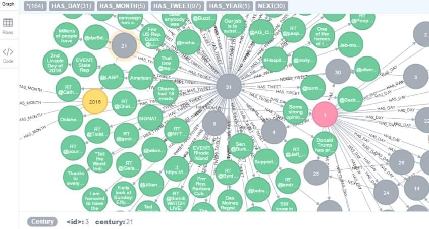
3.3.1 Data Model 1
Figure 3.1 Data Model 121
This is the simplest model among the five models with the time tree on the right to
speed up queries based on time. Figure 3.1 shows the schema. We follow the basic graph
data model guidelines, making nodes for entities and edges to represent relationship between
nodes. For properties like hashtags and urls where multiple of them can occur in a tweet, we
separate them as nodes instead of properties. In the end, we have 5 types of node labels:
Tweet, User, Url, Hashtag and State. Tweet nodes have properties: tweet id which is used to
uniquely identify the tweet, retweet_count (number of retweets of this tweet), retweeted
(whether this tweet has been retweeted by the user), tweet text, created_at (timestamp value
of the tweet posted), day (integer values from 1 to 31), month (integer values from 1 to 12)
and year (2016). Day, month and year values are extracted from the created_at field of the
tweet. Tweet nodes have index on id property. User nodes have properties: user screen_name
(user screen name on Twitter profile), followers (indicating the number of followers) and
following (indicating the number of people this user follows), sub_category (GOP, democrat,
na), category (house_representative, senator, presidential_candidate, senate, reporter) and
name (user full name on Twitter profile). User nodes have indexing on screen_name
property. State and Hashtag nodes have the name property used to indicate the state of the
user and hashtag used by the user with indexing on these two properties. Url has the url
property (expanded URLs used by the User in their Tweets) with indexing on it as shown in
Figure 3.1. The sub_category indicates whether the user belongs to a party, ‘GOP’,
‘democrat’ or ‘na’. The category property value is either senate (for Senate official handlers),
presidential_candidate (for presidential candidates), reporter (for reporters), senator and
house_representative, for senators and house representatives
These nodes are connected with directed edges labeled as shown in Figure 3.1. We
have timeline attached to tweet nodes in data model 1. We use timeline here to show results
of Cypher queries that involve time range [39]. We have generated time tree dynamically
for our study as we do not have the information about the range of years, months and days
to support the tweets in the data model.22
3.3.2 Data Model 2
Figure 3.2 Data Model 2
Figure 3.2 shows the schema of this model. In order to study how performance of the
read-only Cypher query changes, we create new nodes for retweet_count and retweeted
properties of Tweet nodes with indexing on them to observe the effect of increasing the23
number of hops in Cypher queries. Similarly, we create new nodes for the user category and
sub_category properties of the User node with indexing on them. We create an index on
SubCategory nodes to observe the performance when we force queries to use scan by index
instead of scan by label. Apart from this we have indexes on name property of Hashtag, State,
id property of Tweet, url property of Url and screen_name property of User node.
3.3.3 Data Model 3
Figure 3.3 Data Model 3
For our data model 3, we have modified data model 1 and introduced new edges
between hashtag and state and user nodes as shown in Figure 3.3 to compare the performance
of the data models when number of hops are reduced in our Cypher queries. In data model
3, we have indexes on screen_name, id, url and name property of the User, Tweet, Url,
Hashtag and State nodes respectively.24
3.3.4 Data Model 4
Figure 3.4 Data Model 4
This model is the most efficient data model among the four models for most queries.
We designed this data model after analysis of the performance of the first three data models.
It has new SubCategory nodes with the index on the sub_category property and new edges
between state, user and hashtag nodes as shown in Figure 3.4.25
CHAPTER 4
EXPERIMENTAL RESULT AND PERFORMANCE EVALUATION
This chapter describes our data collection methods, performance metrics, evaluation
results of the data models per our metrics, and query results and findings about political
communication.
4.1 Data Collection and Database Creation
We developed two programs in Python 2.7 [52]. We used Neo4j 2.3.3 Community
Edition for Windows [53]. Our first program running in Google App Engine environment
collected tweets using Tweepy 2.3.0 and saved the data into Comma Separated Values (CSV)
format. The second Python program used Py2neo 2.0.9 [54] library to insert the data from
the CSV file into Neo4j to create the database for each data model. This way we can ensure
that all the data models have the same set of data. Figure 4.1 illustrates this process. We ran
our data collection program for 2 days to collect tweets posted since January 1, 2016 till
November 11, 2016. The total number of tweets are 167,671 and they are divided into the
following categories shown in Table 4.1.
Twitter App Tweets
Neo4j DB
Repository Engine CSV
Figure 4.1 Process for importing tweets and related data
Table 4.1. Collected data
Category of Users Number of Twitter Number of tweets collected
handlers
Presidential candidates 10 14,721
Senates 72 50,412
Reporters 45 38,925
Individual senators 88 15,084
House representatives 198 48,52926
Because the graph data models are different, the Cypher queries are also different.
We developed five sets of Cypher queries, one for each data model. Table 4.2 presents the
details about each data model. The number of nodes and edges are not necessarily the same
because we added auxiliary edges and nodes as part of our optimization methods. The
database sizes of the databases with the same number of nodes and edges could also be
different due to whether there were additional schema indexes added to the databases or not.
Table 4.2 Sizes of Data Models
Model 1
(Reference
Model Model) Model 2 Model 3 Model 4
%
Category MBytes MBytes % Change MBytes % Change MBytes Change
Array Store 8 8 0.00 8 0.00 8 0.00
Logical Log 102.48 179.04 74.71 116.91 14.08 109.71 7.06
Node Store 4.13 4.21 1.94 4.13 0.00 4.13 0.00
Property Store 24.66 18.32 -25.71 24.66 0.00 24.66 0.00
Relationship Store 29.88 40.79 36.51 31.51 5.46 31.52 5.49
String Store Size 34.89 34.89 0.00 34.89 0.00 34.89 0.00
Total Store Size 712.88 794.19 11.41 728.87 2.24 719.78 0.97
Number of nodes 288298 294224 2.06 288298 0.00 288305 0.00
Number of edges 661520 997688 50.82 709884 7.31 972136 46.95
4.2 Performance Metric and Measurements
The performance metric is the average query execution time for each query that is
calculated as follows. Each query was run 40 times consecutively on each data model and
the average time for each query was calculated using the last 30 recordings; the first 10 query
response times were not used in the calculation since the execution times were significantly
differences due to cache warm up. In other words, the average performance measured should
be the best case scenario for Neo4j as it may cache the query results. After we finished one
data model, we moved on to measure performance of the next data model until all the data
models were measured. All the queries were executed on the same workstation, an Intel 3.50
GHz CPU with 32 GB RAM running Windows 7 Enterprise 64 bit operating system. We27
used the default server and cache configuration of Neo4j 2.3.3 Community Edition for
Windows in our experiments.
4.3 Experimental Results
We present the comparison of the query response time for all the 25 queries on all
the four data models. Data model 1 is used as the reference model. We summarize the
important findings in Section 4.3.1.
Table 4.3.1 Average time taken by queries in seconds
Model 1
(Reference Model) Model 2 Model 3 Model 4
Query
ID (seconds) (seconds) (% Change) (seconds) (% Change) (seconds) (% Change)
1 0.49497 0.43460 -12.196 0.49607 0.222 0.38997 -21.214
2 0.01527 0.01493 -2.183 0.02053 34.498 0.02013 31.878
3 0.58060 0.59287 2.113 0.14610 -74.836 0.14793 -74.521
4 0.01540 0.00970 -37.013 0.02183 41.775 0.02000 29.870
5 0.00570 0.00533 -6.433 0.00880 54.386 0.00727 27.485
6 0.01460 0.01050 -28.082 0.00437 -70.091 0.00590 -59.589
7 0.00770 0.00437 -43.290 0.00753 -2.164 0.00803 4.329
8 0.00880 0.00810 -7.955 0.00647 -26.515 0.00933 6.061
9 0.08937 0.01190 -86.684 0.08407 -5.931 0.01317 -85.267
10 0.05160 0.04520 -12.403 0.04223 -18.152 0.04853 -5.943
11 0.02900 0.03253 12.184 0.02567 -11.494 0.03137 8.161
12 0.34230 0.32780 -4.236 0.31480 -8.034 0.32937 -3.778
13 2.01973 2.24280 11.044 1.88413 -6.714 2.24417 11.112
14 0.01887 0.01417 -24.912 0.01347 -28.622 0.01637 -13.251
15 0.13313 0.13983 5.033 0.12470 -6.335 0.12190 -8.438
16 0.43363 0.43657 0.676 0.42887 -1.099 0.33210 -23.415
17 0.18100 0.13850 -23.481 0.16570 -8.453 0.14483 -19.982
18 0.18670 0.24623 31.887 0.17530 -6.106 0.18427 -1.303
19 0.17320 0.14023 -19.034 0.16870 -2.598 0.15037 -13.183
20 0.06410 0.06793 5.980 0.06760 5.460 0.07260 13.261
21 0.18810 0.16913 -10.083 0.18913 0.549 0.15163 -19.387
22 0.32360 0.32250 -0.340 0.31247 -3.440 0.30583 -5.490
23 0.41587 0.35467 -14.716 0.42150 1.355 0.33737 -18.876
24 0.41110 0.33777 -17.838 0.39800 -3.187 0.31420 -23.571
25 0.42770 0.44143 3.211 0.42583 -0.436 0.40570 -5.14428 Figure 4.2.1 Comparison of average query response times of Q1-Q9
29

Figure 4.2.2 Comparison of average query response times of Q10-Q17
30

          Figure 4.2.3 Comparison of average query response times of Q18-Q25

                                     4.4. Important Findings
         There is 21.21% improvement for the Q1 in model 4 from model 1 as query scan by
index on the user sub-category property used in model 4 is much faster than query scan by
label in model 1. For Q2, model 2 gives the best performance due to the use of RetweetCount
as nodes is better than the use of the property retweet_count of Tweet nodes.
         For Q3 there is 74.52% improvement in model 4 from model 1 as we have introduced
new edges between the hashtags and the state nodes so the number of hops gets reduced to 1
hop in model 4 compared to 3 hops in model 1.
         For Q6 there is 59.59% improvement in model 4 compared to model 1 even though
in both the models we have scan by index. This is because we have introduced new edges
between user and hashtags used by the user, which resulted in 2 hops instead of 3 hops in
model 1. For Q13, Cypher query is same for model 2, model 3 and model 4 but still model 3
has least query execution time, it is likely due to the fact that model 3 has least number of
edges.
You can also read