Improving an Automated Fog Detection System with Transfer Learning
←
→
Page content transcription
If your browser does not render page correctly, please read the page content below
Improving an Automated Fog
Detection System with Transfer
           Learning
     A Computer Vision Problem

         Michael J. Quinlan

      A thesis presented for the degree of
    Master of Science in Applied Data Science

                Department of Science
                 Utrecht University
                    Netherlands
                     July 2021

       In collaboration with: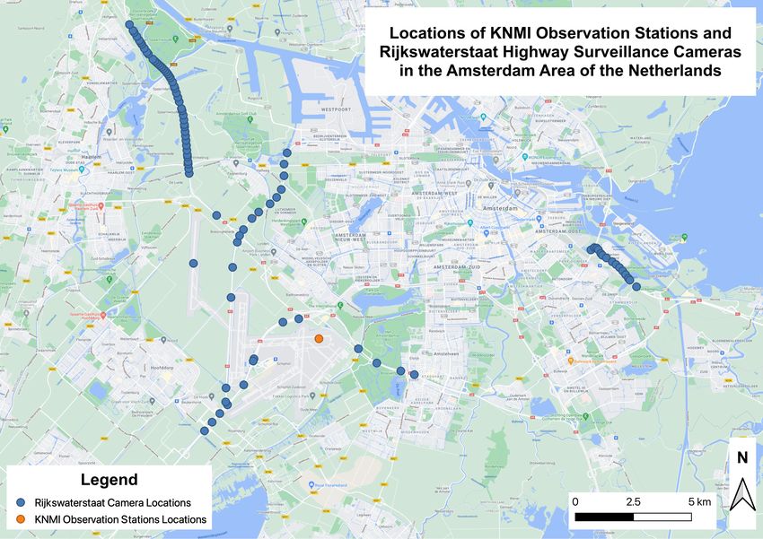
ABSTRACT

   Dense fog conditions can result in transportation disruptions when motorists encounter
significant reductions in visibility. Caution needs to be heeded when these conditions are
experienced and early-warning systems are one of the best defences for alerting motorists
of these conditions. With the prevalence of surveillance cameras along highways to monitor
traffic flow, image data is plentiful as these cameras operate 24/7. With access to this
data, an automated fog detection system has been developed by KNMI that employs a
Convolutional Neural Network (CNN) to classify these images as ’fog’ or ’no fog’. While the
system has been performing satisfactorily with images during daylight hours, the system is
not as robust when it attempts to classify images during nighttime hours.
   Consequently, the aim of this study is to develop the architecture of a CNN that has
satisfactory performance classifying visibility conditions during nighttime hours. One of the
main challenges with this study was the lack of ’fog’ image data as dense fog is a fairly
rare event. Therefore, two approaches were used in this study. The first was to include
some basic data augmentation techniques such as cropping, resizing, rotating, and flipping
images to synthetically increase the dataset. The second approach included implementing
transfer learning to improve the performance of the classifier. A variety of well-known and
high-performing architectures were employed including the use of the VGG16 model. Since
these models were trained on large image data sets, they can be re-used since the features
learned can be transferred to a new domain.
   The VGG16 model emerged as the best performing model from the four pre-trained
models used in this task. Its performance was very similar to the existing model developed
by KNMI. Areas of improvement are need in decreasing the number of false positives as many
images that were identified as fog were not labeled as such. Based on CNN architectures
used in other weather classification tasks, such as classifying clouds, simpler, less complex
network architectures seem to perform the best on this image data set.
   While the strategies adopted for use in this study did not produce a classifier with
better performance than KNMI’s exiting model, the results indicate that this is a challenging

                                              1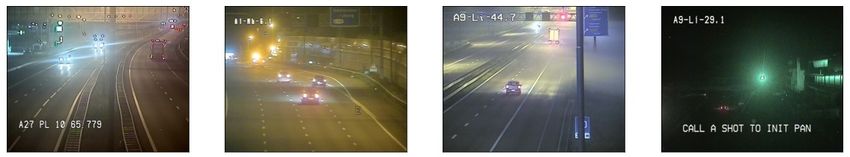
Improving an Automated Fog Detection System with Transfer Learning                 Chapter 0

problem to solve and underscores the need for continued research in this area. Since one of
the main challenges of this problem is the highly skewed image data set to the negative class,
artificially increasing the image data set by employing a Generative Adversarial Network may
help the network learn more features of nighttime fog images.

                                                                                            2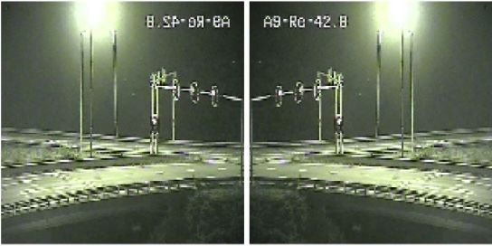
Contents

1 Introduction                                                                                                                                               6
  1.1 Background . . . . . . . . . . . . . . . . . . . . . . . . . . . . . . . . . . . .                                                                     6
  1.2 Problem Statement . . . . . . . . . . . . . . . . . . . . . . . . . . . . . . . .                                                                      8
  1.3 Research Questions . . . . . . . . . . . . . . . . . . . . . . . . . . . . . . . .                                                                     9

2 Data                                                                                                                                                      12
  2.1 Description . . . . . . . . . . . . . . . . . . . . . . . . . . . . . . . . . . . .                                                                   12
  2.2 Preparation . . . . . . . . . . . . . . . . . . . . . . . . . . . . . . . . . . . .                                                                   12
  2.3 Legal and Ethical Concerns . . . . . . . . . . . . . . . . . . . . . . . . . . .                                                                      16

3 Methodology                                                                                                                                               18
  3.1 Convolutional Neural      Networks                .   .   .   .   .   .   .   .   .   .   .   .   .   .   .   .   .   .   .   .   .   .   .   .   .   18
  3.2 Data Augmentation .       . . . . . .             .   .   .   .   .   .   .   .   .   .   .   .   .   .   .   .   .   .   .   .   .   .   .   .   .   21
  3.3 Transfer Learning . .     . . . . . .             .   .   .   .   .   .   .   .   .   .   .   .   .   .   .   .   .   .   .   .   .   .   .   .   .   22
  3.4 Model Evaluation . .      . . . . . .             .   .   .   .   .   .   .   .   .   .   .   .   .   .   .   .   .   .   .   .   .   .   .   .   .   26

4 Experiments                                                                                                                                               30
  4.1 Sample Sets . . . . . . . . . . . . . . . . . . . . . . . . . . . . . . . . . . . .                                                                   30
  4.2 Models Evaluated . . . . . . . . . . . . . . . . . . . . . . . . . . . . . . . . .                                                                    30
  4.3 Model Settings . . . . . . . . . . . . . . . . . . . . . . . . . . . . . . . . . .                                                                    31

5 Results                                                                                                                                                   33
  5.1 Validation Results . . . . . . . . . . . . . . . . . . . . . . . . . . . . . . . . .                                                                  33
  5.2 Test Results . . . . . . . . . . . . . . . . . . . . . . . . . . . . . . . . . . . .                                                                  35

6 Conclusion                                                                                                                                                38
  6.1 Overall Findings . .      .   .   .   .   .   .   .   .   .   .   .   .   .   .   .   .   .   .   .   .   .   .   .   .   .   .   .   .   .   .   .   38
  6.2 Discussion . . . . . .    .   .   .   .   .   .   .   .   .   .   .   .   .   .   .   .   .   .   .   .   .   .   .   .   .   .   .   .   .   .   .   39
  6.3 Study Limitations . .     .   .   .   .   .   .   .   .   .   .   .   .   .   .   .   .   .   .   .   .   .   .   .   .   .   .   .   .   .   .   .   40
  6.4 Further Study Areas       .   .   .   .   .   .   .   .   .   .   .   .   .   .   .   .   .   .   .   .   .   .   .   .   .   .   .   .   .   .   .   42

A Appendices                                                                                                                                                43

                                                                3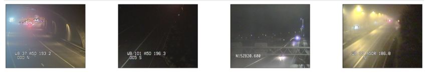
List of Figures

 1.1   Surveillance Cameras Available to KNMI in the Amsterdam Area . . . . . .                                                       7
 1.2   Image Source Locations in the Netherlands . . . . . . . . . . . . . . . . . . .                                                8

 2.1   Distribution of Class Labels . . . . . . . . . .          . . . . . .             .   .   .   .   .   .   .   .   .   .   .   13
 2.2   Distribution of Phase Labels . . . . . . . . . .          . . . . . .             .   .   .   .   .   .   .   .   .   .   .   14
 2.3   Fog and No Fog Sample Images for Illustrative             Purposes                .   .   .   .   .   .   .   .   .   .   .   15
 2.4   Creation of Image Data Sets . . . . . . . . . .           . . . . . .             .   .   .   .   .   .   .   .   .   .   .   16

 3.1   Example Convolutional Neural Network .        .   .   .   .   .   .   .   .   .   .   .   .   .   .   .   .   .   .   .   .   21
 3.2   Example Horizontal Flip . . . . . . . . .     .   .   .   .   .   .   .   .   .   .   .   .   .   .   .   .   .   .   .   .   21
 3.3   Transfer Learning . . . . . . . . . . . . .   .   .   .   .   .   .   .   .   .   .   .   .   .   .   .   .   .   .   .   .   23
 3.4   VGG16 Base Model . . . . . . . . . . . .      .   .   .   .   .   .   .   .   .   .   .   .   .   .   .   .   .   .   .   .   24
 3.5   Classification Architecture . . . . . . . .   .   .   .   .   .   .   .   .   .   .   .   .   .   .   .   .   .   .   .   .   25
 3.6   ODuring Training and Validation . . . .       .   .   .   .   .   .   .   .   .   .   .   .   .   .   .   .   .   .   .   .   26
 3.7   Precision-Recall Curve . . . . . . . . . .    .   .   .   .   .   .   .   .   .   .   .   .   .   .   .   .   .   .   .   .   29

 5.1   Precision-Recall Curve for Night Image Dataset                .   .   .   .   .   .   .   .   .   .   .   .   .   .   .   .   34
 5.2   Confusion Matrices Comparison . . . . . . . . .               .   .   .   .   .   .   .   .   .   .   .   .   .   .   .   .   36
 5.3   Sample of False Negative Images . . . . . . . . .             .   .   .   .   .   .   .   .   .   .   .   .   .   .   .   .   36
 5.4   Sample of False Positive Images . . . . . . . . .             .   .   .   .   .   .   .   .   .   .   .   .   .   .   .   .   37
 5.5   Receiver Operating Curve for Test Set . . . . .               .   .   .   .   .   .   .   .   .   .   .   .   .   .   .   .   37

 6.1   Challenging Images to Label . . . . . . . . . . . . . . . . . . . . . . . . . . .                                             41
 6.2   Incorrectly Labelled and Challenging Images . . . . . . . . . . . . . . . . . .                                               41

                                             4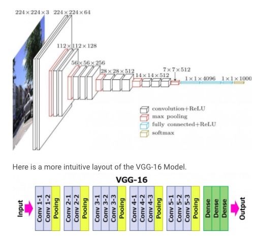
List of Tables

 2.1   Re-coding Day Phases . . . . . . . . . . . . . . . . . . . . . . . . . . . . . .   14

 3.1   Pretrained Models Used with Number of Trainable Parameters . . . . . . . .         23

 4.1   Composition of Balanced Dataset . . . . . . . . . . . . . . . . . . . . . . . .    30
 4.2   Composition of Imbalanced Dataset . . . . . . . . . . . . . . . . . . . . . . .    30

 5.1   Model Evaluation Results for the Night Image Dataset . . . . . . . . . . . .       33
 5.2   Model Evaluation Results for the Night Image Dataset . . . . . . . . . . . .       35

 6.1   Comparison of Trainable Parameters and F1-Scores . . . . . . . . . . . . . .       39
 6.2   Model Evaluation Results for the Night Image Dataset . . . . . . . . . . . .       40

                                            5
1      Introduction
    To orient readers, an introduction has been provided which provides background infor-
mation regarding the problem and what has been done to date to solve it. Further, this
section describes the problem and its scope which leads to an identification of the primary
research questions that were used as a focal point for this study.

1.1      Background
    Fog is a difficult meteorological phenomenon to predict and can result in high-impact,
short-lived weather events that may cause serious travel impairments [25]. Therefore, there
is a need to predict and identify fog conditions quickly to provide critical information to the
public and to those working in transportation industries that rely on visibility for navigational
purposes.
    Essentially a low elevation cloud, fog is composed of water droplets and obscures the
landscape to varying degrees which can lead to flight cancellations and/or car accidents. Fog
often occurs when cold air is located just above a relatively warm and moist surface. Due
to a density difference, the warm and moist air at the surface rises into the relatively cold
air above and condenses onto atmospheric particles such as ash and dust resulting in the
formation of a cloud at the surface [25]. While there are several fog formation mechanisms,
each with their own set of parameters, their individual names and characteristics are beyond
the scope of this paper.
    The fleeting and localized nature of fog makes it a difficult weather phenomenon to
forecast far in advance [2]. Most numerical weather prediction models, with their coarse-grid,
have difficulty forecasting such a fine-grid, localized phenomenon[2]. Fog often occurs due
to terrain and land cover features, thus one location can have significantly lowered visibility
while other nearby locations may not. Additionally, fog conditions can change rapidly in
time with an area experiencing dense fog at one moment followed by dramatic clearing
[19] [2]. The current methods for observing fog conditions, such as expensive sensors and

                                               6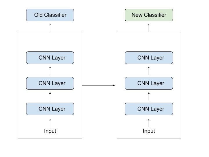
Improving an Automated Fog Detection System with Transfer Learning Chapter 1
human-beings, are limited in their observational areas; thus, other methods that are more
comprehensive in their observational area are needed in order to quickly and accurately warn
the public of its presence on roadways [25].
Traditionally, fog detection has been performed by using human observers or equipment
located at official weather observing stations including airports [27]. The primary limitation
of making fog observations this way is the lack of extensive spatial coverage. Additionally, it
is unfeasible to observe weather conditions this way given the resources needed to support a
network of humans and high-cost machines [21]. However, traffic monitoring cameras have
been installed by the Rijkswaterstaat [21] across the Netherlands and offer a low-cost solution
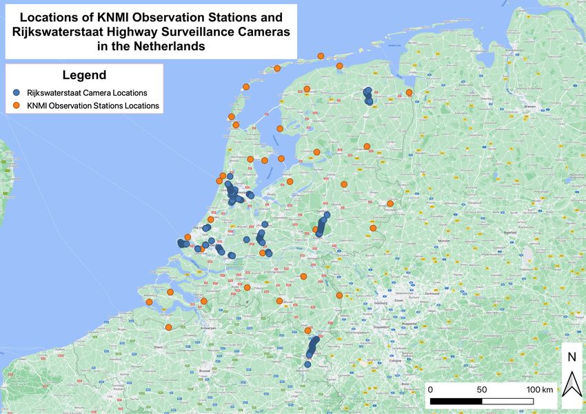
to collect weather data since the cameras are already installed and widely distributed. Figure
1.1 is an example from the Amsterdam area and nicely shows the discrepancy between official
weather observation stations (the one orange circle in the center of the image) and traffic
monitoring cameras.
Figure 1.1: Surveillance Cameras Available to KNMI in the Amsterdam Area
To remedy this discrepancy, KNMI has partnered with the Rijkswaterstaat to access
imagery captured by some of their traffic surveillance cameras which are distributed widely
across the Netherlands [21]. Example locations of highway cameras that are accessible to
KNMI are shown in figure 1.2. These surveillance cameras have provided vast amounts
7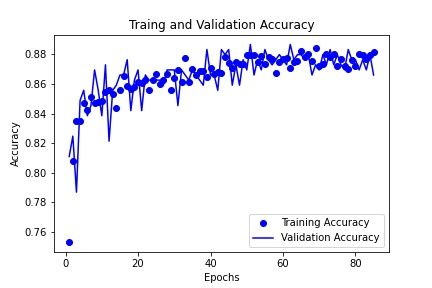
Improving an Automated Fog Detection System with Transfer Learning                  Chapter 1

of image data to KNMI which has used it to automatically identify fog conditions during
daylight hours [21]. Moving forward, KNMI’s focus is on enhancing the automated fog
identification system by extending its ability to times of the day when there is little-to-no
natural sunlight (i.e., dawn, dusk, and overnight hours) [21].

                  Figure 1.2: Image Source Locations in the Netherlands

1.2     Problem Statement
   Applications of CNN are occurring in many domains including underwater identification
of objects, cloud classification, and medical diagnosis [10]. Some of the challenges experi-
enced in these areas, with respect to image quality (low-contrast, low-light situations) and
imbalanced data sets are similar to those that KNMI are hoping to address. The successes
achieved in these domains may be extended to address the issue of image quality in nighttime
fog detection.
   Compared to the typical image classification task, weather classification from images is
affected by various factors, e.g., illumination, reflection, dispersion and shadow [9]. Each of
these optical effects interact with one another resulting in dependencies among each other
which are difficult to untangle. According to Elhoseiny, Huang, and Elgammal [9], ”al-

                                                                                             8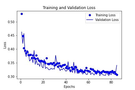
Improving an Automated Fog Detection System with Transfer Learning                  Chapter 1

though the previous engineered approaches can satisfy some desirable properties and mitigate
some undesirable properties from these factors, they cannot well capture such non-linearity
of the categorization manifold, which makes discrimination between weather classes a hard
problem.”
   To date, computer vision is making huge strides in solving many problems related to
meteorology. However, one major challenge remains: access to data that represents all the
variety of outdoor conditions that can exist, from diurnal changes in sunlight to changes in
weather conditions. For example, in this project there is huge disparity between the number
of ’fog’ images compared to the number of ’no fog’ images; the dataset is heavily imbalanced
toward ’no fog’ images. Creating a successful strategy to generating synthetic images of ’fog’
conditions to increase the dataset is a step toward resolving this challenge.
   As noted earlier, fog can be a hazardous weather phenomena that can occur and dissi-
pate quickly [25], thus the automated fog detection system could communicate fog conditions
to “smart” transportation operators who can provide this information to motorists via ad-
justable speed limit and warning signs, or possibly directly to motorists via their in-car
navigation systems. These can be used to alert motorists of visibility reductions and can
guide them to a proper speed limited.
   Therefore, the successful development of a neural network capable of accurately identify-
ing fog conditions could be useful to other researchers in the computer vision field. A network
that is trained to identify fog conditions during nighttime hours, and perhaps even estimate
visibility under these conditions, could be used in any “smart” transportation system to
mitigate the risks involved in driving during low-visibility weather conditions.

1.3     Research Questions
   An automated system has already been established by KNMI that uses a deep learning
neural network capable of identifying fog conditions using traffic camera imagery during
day light hours. KNMI has defined fog conditions as those when ‘visibility is less than 250
meters’ [22] which is considered ”dense/heavy fog” - a relatively infrequent (but potentially
high-impact) meteorological event [12]. Fog conditions monitored by visibility detectors at
weather stations are limited, however, highway surveillance cameras are plentiful and can fill

                                                                                             9
Improving an Automated Fog Detection System with Transfer Learning Chapter 1
the gap in identifying hazardous driving conditions.
While the day time model has proven successful, the nighttime model has not yet shown
satisfactory performance with a precision score of 77% and a recall score of 87% [21]. The
challenge is to improve theses scores since the dataset is severely imbalanced and weighted
more toward the non-fog class. This could be done artificially by simply changing the thresh-
old of what is considered a fog image (currently set at 0.50 with values greater indicating
’fog’.) However, since dense fog is a relatively rare event that could have significant and
dangerous consequences if not identified accurately, the goal is to detect as many of these
anomalous events as possible.
There are two main challenges that need to be addressed to improve the performance of
the nighttime automated fog detection system. First, the training set of real fog conditions
during nighttime hours is limited and highly-unbalanced (for every 1 fog image, there are
24 non-fog images) [21]. This makes training the network difficult as neural networks are
“data hungry” requiring very large training sets properly balanced between the classes to be
recognized to avoid over-fitting [5]. The second problem is the poor quality of the nighttime
images. During nighttime hours, artificial lighting is used to illuminate the roadways and
this can add noise to the images and decreases the contrast. Additionally, the fine particles
that make up fog tend to scatter and absorb light resulting in decreased image quality as
[19] these interactions tend to distort the images [19].
However, according to Pagani, Noteboom, and Wauben [21], deep neural networks are
good in adapting to the changing scenery for surveillance cameras, as these cameras are
independently operated and each camera might be tuned to different settings. To account
for this, the main objectives of this research project is to apply transfer learning to a baseline
classification model and evaluate its performance in comparison to the current model used
by KNMI.
The main research question that drove this study is as follows:
What training strategies can be employed to improve the performance of a
binary classifier for fog detection on small and imbalanced data sets?
CNNs include many different hyper-parameters and consist of several layers stacked upon
each other, therefore there are many choices that could be made to fine-tune the model [24].
10Improving an Automated Fog Detection System with Transfer Learning Chapter 1
In this study, two strategies were employed to aid in the classification of ’fog’ and ’no fog’
images at night, data augmentation and transfer learning. Additionally, several evaluation
metrics for this task were used to determine which is the best performing model.
Therefore, the following three sub-questions were also explored:
1. Can data augmentation techniques such as cropping, flipping, and resizing
images improve the performance the fog detection system?
2. Can a pre-trained convolutional network such as the VGG16 be used to
improve the performance of the fog detection system?
3. Which evaluation metrics are best suited for a binary classification prob-
lem such as classifying fog given a small and imbalanced dataset?
Strategies to accomplish this are outlined in the Methodology section of this paper.
112 Data
In this chapter, a description of the dataset is provided along with the data preparation
and wrangling steps used to create sample data sets, and finally a nod to the potential legal
and ethical issues involving the use of public data is provided.
2.1 Description
The data provided for use in this study was in the from of camera imagery obtained
from Rijkswaterstraat’s highway surveillance cameras. Additionally, annotation files were
generated which contained metadata on the images including filename, camera ID, location,
timestamps, and each image’s corresponding labels (i.e., ’fog’, ’nofog’, ’cannot say’.) An
additional attribute called ’day phase’ was also included that identified the period of the day
during which the image was taken. This was used to separate the day images from the night
images.
2.2 Preparation
The image data set included 54,213 samples while the annotations file contained 54,714
samples. Given the disparity in the number of images and annotations, 501 duplicate an-
notations were identified and removed from the annotations file. This was accomplished by
employing an inner join on the two data frames via the filename field. Further, 2,968 images
labelled ’cannot say’ were removed from the data set since this is a binary classification
problem focused on ’fog’ and ’no fog’ images. Of the remaining 51,245 images, 49,230 were
labeled as ’no fog’ images and the remaining 2,015 images were labeled as ’fog’ as shown
in figure 2.1. Finally, no missing data was found in the annotations file and all images
referenced were accounted for.
12Improving an Automated Fog Detection System with Transfer Learning Chapter 2
(a) Before Data Wrangling (b) After Data Wrangling
Figure 2.1: Distribution of Class Labels
As clearly visualized in 2.1, this is a highly imbalanced data set with approximately 1
’fog’ image for every 24 ’no fog’ images. An imbalanced data sets is a common challenge for
CNNs to overcome. Several strategies have been identified to address this problem including
randomly under-sampling of the majority class, which was employed in this case [5]. Under-
sampling the majority class was was chosen so that the evaluation metric, accuracy, could be
used without misinterpretation. While this is a common strategy for training a network on
an imbalanced dataset, a known problem with this approach is information loss [5]. Images
not used contain information that might be helpful to learn the mapping between inputs and
outputs but this lost information cannot be recovered.
From a meteorological perspective, it makes sense that there are more ’no fog’ images
than ’fog’ images as fog is a relatively rare event [12]. This is particularly acute in this study
as the operational definition that KNMI used to label ’fog’ images is visibility less than 250
meters [22]. This type of fog event is called dense fog which is rarer than ”lighter” fog event
[12].
As previously mentioned, the feature ’day phase’ was also included in the annotation files
to identify the time of day. The classes for day phase included civil dusk and dawn, nautical
dusk and dawn, astronomical dusk and dawn and simply, night and day. Since the cameras
use visible light for taking photos, ’day’ was operationally defined as those times of the day
when the there is enough sunlight that other sources of light are not needed for illumination
[13]. This corresponds to the day phases labeled as civil dawn and dusk. Therefore, those
13Improving an Automated Fog Detection System with Transfer Learning Chapter 2
classes were re-coded simply as ’day’, and the remaining classes, nautical and astronomical
dawn and dusk were re-coded as ’night’ as shown in table 2.1. In accordance with the
classification task, re-coding to ’day’ and ’night’ was performed to differentiate ’day fog’
images from ’night fog’ images. The result of this re-coding and aggregation is a distribution
of 28,185 day images and 23,060 night images with approximately 1 night image for every
1.2 day images.
Numeric Code Description Reassigned Phase
0 Night Night
1 Day Day
10 Civil Dawn Day
11 Civil Dusk Day
20 Nautical Dawn Night
21 Nautical Dusk Night
30 Astronomical Dawn Night
31 Astronomical Dusk Night
Table 2.1: Re-coding Day Phases
The result of this re-coding is shown in the distribution of day and night images shown
in figure 2.2.
(a) Before Data Wrangling (b) After Data Wrangling
Figure 2.2: Distribution of Phase Labels
To train and evaluate a CNN to classify ’fog’ and ’no fog’ images at night, a balanced
dataset totalling 4,030 samples from the population dataset was created using the number
of ’fog’ images, 2015, as the limiting factor. The night subset was composed of 4,908 images
14Improving an Automated Fog Detection System with Transfer Learning Chapter 2
of which 1,454 were ’fog’ and 1,454 were ’no fog’. Each subset, ’fog’ and ’no fog’ images
were further divided into training, validation and testing subsets based on the following
percentages: 80% for training, 10% for validation, and 10% for testing. The training set for
’night’ images included 1,158 ’fog’ images and 1,158 ’no fog’ images. The validation set for
’night’ images included 143 ’fog’ images and 148 ’no fog’ images. The test set for ’night’
images included 153 ’fog’ images and 138 ’no fog’ images. The balanced data set was used
to train and validate the models used in this study. The balanced dataset was also used to
evaluate overall model performance to determine which performed the best.
To test the best model under a more realistic scenario, when there are more ’no fog’
images than ’fog’ images, a balanced test set was created as well. This set had to be
carefully constructed to not include images previously used for training and validating the
models. The original 153 ’fog’ test set images were used and a new 3,000 ’no fog’ were taken
from the night sample as there are an abundance of night, ’no fog’ images. This test set that
was then used on the best model architecture developed for this project and on the model
already developed at KNMI.
For illustrative purposes, four samples of nighttime images labeled as ’fog’ are shown in
figure 2.3a along with four samples of nighttime images labeled ’no fog’ shown in figure 2.3b.
(a) Fog Samples
(b) No Fog Samples
Figure 2.3: Fog and No Fog Sample Images for Illustrative Purposes
To aid in understanding how the sample subsets for training, validation, and testing were
formed, a visualization is shown in figure 2.4.
15Improving an Automated Fog Detection System with Transfer Learning Chapter 2
(a) Balanced Data Sets (b) Imbalanced Data Sets
Figure 2.4: Creation of Image Data Sets
2.3 Legal and Ethical Concerns
As governmental organizations, both KNMI and Rijkswaterstaat adjere to the Nether-
lands’ government Open Data policies that allow free use of data by the public [18]. While
these organizations allow public use of data, some data cannot be made publicly available
due to privacy concerns. This is true for the images used in this study as they may include
private citizen information such as license plate numbers, vehicle make and model, and even
faces. While license plate numbers and individual faces were not visible by eye in any of
the images viewed, it remains a possibility that private citizens could be identified via these
images. Therefore, KNMI complies with the European Union’s privacy law known as Gen-
eral Data Protection Regulation (GDPR). The GDPR requires a justification of the use and
handling of private data. Data that includes private information may still be used, but the
16Improving an Automated Fog Detection System with Transfer Learning Chapter 2
data must be registered and individuals using the data must be authorized to do so [17].
In this case, Rijkswaterstaat granted access to the images for a limited amount of time for
research purposes.
In terms of ethical concerns, the goal of this project is to improve an automatic fog
detection system so that motorists are forewarned of potential hazardous driving conditions.
Hazardous driving conditions can result in accidents, injury, or even death, thus this project
aims to benefit motorists. Therefore, the outcomes of this project are purely to increase
safety on the roadways. Ultimately, this is a public service project aimed at protecting the
public, a noble goal with only a positive impact on society.
173 Methodology
There are two main challenges associated with this image classification task that need to
be resolved in order to develop a model that is capable of accurately identifying dense fog
conditions at night. First and foremost is the reality that the dataset is small especially in
the case of the positive cases (i.e., ’fog’ images) which limits the amount of learning that the
model can achieve and potentially causes false impressions about the model’s performance
[11]. The second hurdle is image quality due to poor and inconsistent lighting conditions
that cause the images to be very noisy, and for any weather classification task, the images
are affected by observed conditions such as illumination, reflection, and dispersion of light
[9]. These challenges motivated the choices made in developing a CNN for this task.
3.1 Convolutional Neural Networks
Convolutional Neural Networks are a type of deep learning that are particularly good at
image classification and thus will be used to address this problem [24], [7] [3]. On a very
basic level, CNNs work by taking an input image and mapping it to a particular output
class [24], [7] [3]. Since the dataset includes labeled images, this is considered a supervised
learning problem.
In our case, the input data is an image which is represented by pixel values stored in a four
dimensional tensor. These images have four dimensions associated them: batch size, width,
height, and channels, where the channels represent the type of image [24], [7] [3]. A channel
value of ’1’ indicates a grayscale image and a channel value of ’3’ indicates a color image [i.e.,
red, green, and blue channels]. These values are stored in arrays which are manipulated via
mathematical operations including convolution, averaging, pooling, resizing, etc [24], [7] [3].
Here, the the output is a probability value indicating the image’s membership to the ’fog’
class. If the probability value is greater than 0.50, the image is classified as ’fog’. Conversely,
if the probability value is less than or equal to 0.50, the image is classified as ’no fog’. It is
important to note that the threshold value is arbitrarily chosen and can be adjusted based
18Improving an Automated Fog Detection System with Transfer Learning Chapter 3
on the problem at hand. This technique has been shown to be effective when improving
the performance of a classifier on a skewed data set [23]. There may be times when it is
necessary to have a high threshold value, which may limit the number of positive cases, but
potentially identifies the cases that are, without a doubt, positive. In other cases, it may
be necessary to be more lenient. Then, the threshold value would be lowered to allow other
cases with more uncertainty to belong to the positive class.
How the CNN determines the mapping between input and a output relies on the use of a
perceptron and a non-linear activation function [3] and [7]. The perceptron acts as a linear
boundary separating classes from one another [3] and [7]. The coarsest perceptron would
simply be a line drawn through the perceived middle of all the data points. However, using
only linear separators would lead to generalization where the model is too liberal with its
boundary and is not considering the non-linearity that naturally exists in image data [24],
[24], [7] and [3].
Activation functions provide a means of curving the perceptron to add more nuance to the
separation boundary [3] and [7]. Consider water flowing down a mountain: the most direct
route is a straight line from origin to destination, but water flowing down a mountain does
not behave that way. Rather, it twists and turns dependent on the topology it interacts with,
ultimately finding the easiest path to traverse. In a similar way, activation functions provide
this mathematical twisting and turning to reduce the error in determining the boundary
between classes [3] and [7]. The activation function used here was the ReLU function which
is common for CNN architectures and has outperformed other activation functions such as
tanh and sigmoid [3] and [7]. The ReLu function is simple to understand; it forces any value
less than 0 to be 0 and any value greater than 0 to be 1 [3] and [7].
In this study, a sequential CNN model was built with layers stacked upon each other
one after the other [3] and [7]. Most CNNs are composed of the following layers: input,
convolutional, activation, pooling, dropout, flatten, and dense [3] and [7]. Each layer in the
network serves a particular purpose in the process of mapping input image to output class.
The convolutional layers are used for feature extraction where a known feature filter
known as a kernel is slid across the image from left-to-right and top-to-bottom to determine
if the feature is contained within the image [7] and [3]. Pooling layers are used to aggregate
19Improving an Automated Fog Detection System with Transfer Learning Chapter 3
the properties in a region of the image [7] and [3]. Since images are composed of pixel
data, the amount of data in an image can be tremendous and is dependent on its size and
resolution. The pooling layer simply performs a mathematical operation such as ’average’
or ’sum’ on the region of interest and returns one value representing that region [7] and [3].
While this cause information loss, there is so much information in an image that it is close to
negligible [7] and [3]. Consider, for example, the impressionist paintings produced by Claude
Monet in the late 1800s. Objects are clearly distinguishable yet they are made up of coarse
strokes compared to fine strokes.
Dropout layers were included to reduce the number of weights that the network has to
learn and and, in turn, prevent the network from over-fitting [7] and [3]. The choice behind
including dropouts is to reduce the number of activations that occur in the network [3] and
[7]. Over-fitting occurs when the model has learned too much from the training data (almost
memorizing it) and thus it performs poorly on unseen data as it expects the same complex
pattern [7] and [3]. A typical signature of over-fitting is when the training accuracy exceeds
the validation accuracy.
The final portion of the models, where the classification took place, were made up of
fully-connected flatten and dense layers. Flattening simply transforms a multi-dimensional
array into a one dimensional vector [7] and [3]. It is used so that the multi-dimensional
image data can be mapped to one dimensional output [3] and [7]. In this case, a probability
value indicating the image’s class membership. Being fully-connected every output from the
previous layer is mapped to a specific output in the following layer [7] and [3]. No neurons
(where the activation functions are located) are skipped. The sigmoid activation function
was used since it is a logistic function producing either a ’0’ for negative class (’no fog’)
or ’1’ for the positive class (’fog’) [7] and [3] and is commonly used in binary classification
tasks. Here, the output layer consisted of one neuron with an attached probability value. As
indicated previously, if the probability value returned was greater than 0.5, the image was
assigned to the positive, ’fog’ class, otherwise it was assigned to the negative, ’no fog’ class.
An example of a CNN used for binary classification is shown in figure 3.1 minus dropout
layers.
20Improving an Automated Fog Detection System with Transfer Learning Chapter 3
Figure 3.1: Example Convolutional Neural Network
3.2 Data Augmentation
Data augmentation is used in many image classification tasks especially when the dataset
is limited in volume [16]. The effect of implementing data augmentation is to synthetically
increase the training data set so that the network can learn from more samples [7] and [3].
There are many flavors of data augmentation that can be applied from cropping, rotating,
flipping, resizing, and zooming to name a few. Each of these techniques can be applied to
one image to create additional training images. As with any technique used, it must be
appropriate for the data at hand. In this study, it would not make sense to vertically flip
the images since this would force the roadway to be at the top of the image. This could
potentially cause the model to learn incorrect mappings. Data augmentation used in this
study included horizontal flipping, rotation (max. 40), brightness increases, resizing and
zooming.
An example of a horizontally flipped image is shown in figure 3.2.
Figure 3.2: Example Horizontal Flip
21Improving an Automated Fog Detection System with Transfer Learning Chapter 3
3.3 Transfer Learning
Transfer learning was chosen as a method to improve model performance since it is a
widely used technique in deep learning especially when dealing with anomalous events and
small data sets [7] and [3]. Training a neural network requires a significant amount of data
to map input to output, therefore, when working with a small data set, transfer learning is
often used [14]. Effectively, transfer learning refers to using the parameter weights learned
from previous classification tasks and applying them to a new domain [7] and [3]. When
the data set is small and transfer learning is not employed, the learned mappings tend to
over-fit the data resulting in less generalization of the model. Therefore, by incorporating
the mappings learned from previous image classification tasks, over-fitting is less likely to
occur [20] and [14].
The main challenge associated with using transfer learning to improve model performance
is choosing the right model [7] and [3]. While the decision can be aided by reviewing the
classification tasks upon which the model was originally trained, often its a case of trial-by-
error [7] and [3].
The process involved in transfer learning includes downloading the architecture for the
existing model along with its learned weights [7] and [3]. These layers serve as the convolu-
tional base of the model and are involved in the feature detection and extraction processes
that occur in the convolutional layers [7] and [3]. Since these features have already been
learned via training on other data sets, it is computationally inexpensive when compared to
a model that has to learn the features first and then detect them [7] and [3].
The convoultional base layers from the pre-trained model are ’frozen’ so that the weights
learned in previous classification tasks are not overwritten and they can be applied to the
new problem [7] and [3]. In this case, the convoluational base model was topped-off with
trainable, fully-connected layers that serve as the classification portion of the model. These
fully-connected layers were chosen based on the CNN architecture that was used in the ’Cats
and Dogs’ classification task [7] and [3]. A visual of using a pre-trained is shown in 3.3.
22Improving an Automated Fog Detection System with Transfer Learning Chapter 3
Figure 3.3: Transfer Learning
To identify a ”best model”, four different well-known CNN architectures were evaluated
separately for the night image dataset. Each model is listed and described briefly in table
3.1 along with each model’s number of trainable parameters.
Model Description Trainable
Parameters
VGG16 VGG16 (5 blocks) as convolutional base with 3,211,521
binary classification layers added
InceptionV3 Inception as convolutional base with binary clas- 134,219,777
sification layers added
ResNet50 Resnet50 as convolutional base with binary clas- 23,587,712
sification layers added
EfficientNetB0 EfficientNetB0 as convolutional base with bi- 21,235,713
nary classification layers added
Table 3.1: Pretrained Models Used with Number of Trainable Parameters
23Improving an Automated Fog Detection System with Transfer Learning Chapter 3
These four architectures were chosen based on their performance on previous classification
tasks and their ease of implementation via Keras-Tensorflow. For example, the VGG16
model shown in figure 3.4 was chosen due to its superior performance in the ILSVRC 2014
Conference where it beat the ’gold standard’ at the time known as AlexNet [7] [3].
Figure 3.4: VGG16 Base Model
Since then, the VGG16 model has been used extensively as a transfer learning model by
applying its known weights to new domain classification problems [14]. As shown below,
this sequential model (a model with layers stack on top of each other where the output of
one layer becomes the input for the following layer) consists of five blocks, each containing
convolutional and pooling layers [7] [3]. The dense layers, where the classification takes place,
were replaced by the classification architecture shown in figure 3.5, which were developed
for one output parameter (probability value). This replacement was necessary as the model
was originally trained on the ImageNet dataset consisting of 1,000 classes [7] [3] in this case,
we only have two classes. The fully-connected layers in the classification portion include one
flatten layer with an output size of 25,088, followed by a dense layer with output size of 128,
and finally an output layer of 1 output [7] [3] .
24Improving an Automated Fog Detection System with Transfer Learning Chapter 3
Figure 3.5: Classification Architecture
After training each model, two evaluation metrics were collected, accuracy and loss for
both the training dataset and the validation. These metrics helped to identify if the model
is over- or under-fitting [7] [3]. In the case of over-fitting, the model is learning too well the
non-linear mappings between input and output variables to such a degree that the patterns
identified cannot be used on unseen data since the model will expect the mappings to be
identical [7] [3]. This leads to continued increases in training accuracy while the validation
accuracy remains stable or, in some cases, decreases.
Alternatively a model that under-fits the data is generalizing too well and is not learning
some of the specific patterns that exist between the input and output variables [7] [3]. Thus,
when the model is used with new data, its performance is poor because it cannot apply some
of the nuances it has learned to the new set of data. Finding this balance is challenging
but analyzing the accuracy and loss data for both the training and validation data helps [7]
[3]. The accuracy and loss curves for the VGG16 model are shown in figure 3.6 and depict
a model that is not over or under-fitting; rather convergence occurs with the accuracy and
loss values reaching the same value during training.
25Improving an Automated Fog Detection System with Transfer Learning Chapter 3
(a) Loss Curve (b) Accuracy Curve
Figure 3.6: ODuring Training and Validation
To prevent over-fitting, a regularization technique known as ’early stopping’ was used to
force the model to terminate once a particular threshold was met [7] [3]. In this case, the
parameters were set to the following values: monitor = val loss, min delta = 0, mode
= ’auto’, patience=7. By setting monitor to val loss, we use the validation loss as the
performance metric to stop the model. Additionally, setting min delta to 0, the mode to
auto, and the patience to 7 forces the model to stop when the validation loss shows no
improvement after seven epochs. These values were chosen based on a visual inspection of
the loss and accuracy data. The resulting ’best model’, the one with the least validation
loss, was identified at epoch 85.
3.4 Model Evaluation
Since this is a binary classification problem for an unbalanced data set with the majority
of images in the negative class and the minority of the images in the positive class, the
best metrics to use for measuring the classifier’s effectiveness include precision, recall, and
F1-score [15] [1]. These metrics are important in this case because they describe how well
the classifier is able to detect images that belong to the positive, minority class.
While accuracy is a popular metric for evaluating a binary classifier’s performance, it
is not a good evaluation metric when dealing with an imbalanced dataset [15] [1]. A high
accuracy score for an unbalanced data set with ’fog’ as the positive class and ’no fog’ as
the negative class could simply indicate that the classifier correctly identified all of the ’no
26Improving an Automated Fog Detection System with Transfer Learning Chapter 3
fog’ images but did not correctly identify any of the ’fog’ images. For example, an accuracy
value of 95% for a data set consisting of 95 ’no fog’ images and 5 ’fog’ images could indicate
that 95 negative cases were identified properly as ’no fog’, but the remaining 5 positive cases
were also identified as ’no fog’. In that case, the classifier would not be able to identify dense
fog and thus, the public would not be warned of hazardous driving conditions - the exact
opposite of KNMI’s goal.
Therefore, for each of the four models developed, precision, recall, and F-1 score values
were the driving force for identifying the best performing model. Since there exists a trade-
off between precision and recall values, by describing one, the other is also described [15]
[1]. For example, a high precision value indicates a low recall value and vice-versa. Since we
would like both values to be high, the additional metric called the F1-score is used which
combine these scores into one score that describes how well the classifier is performing [15]
[1]. An F1-score value close to one indicates that both the precision and recall values are
good [15] [1]. On the other hand, an F1-score close to zero indicates that either precision or
recall is very low and further investigation is needed to determine the cause [15] [1].
To determine which metric is responsible for creating a low F1 score, it is necessary to
examine the number of false positives (Type I error) and false negatives (Type II error) [15]
[1]. This can easily be achieved by producing a confusion matrix that compares the predicted
class label to the actual class label and tallies the number of samples identified correctly and
incorrectly for each class.
False positives can be harmful in situations where being predicted as belonging to the
positive class requires a high-stakes remediation. For example, if the automatic fog detection
system consistently returns false positive values indicating the presence of dense fog when
dense fog is not observed, then motorists would be falsely warned of this weather condi-
tion, and then the motorists may potentially ignore future warnings if false warnings occur
frequently.
Just as harmful, false negatives also need to be monitored as a high value for this metric
indicates that the positive class was not identified correctly. In the case of fog detection, if
dense fog conditions exist at a distance too far from the motorist to observe and the motorist
is not warned of this hazardous driving condition, they could continue driving at their normal
27Improving an Automated Fog Detection System with Transfer Learning Chapter 3
speed and may potentially end up in an accident, or worse, since they were not forewarned
of the dangerous driving conditions.
Therefore, since this is a highly imbalanced data set with 1 ’fog’ image for every 24
’no fog’ images, the following evaluation metrics were used to identify the best performing
classifier among the seven models developed.
• False Positive Rate: a ratio of the number of false positive samples to the sum of
the false positives and true negatives [4]. See equation (3.1)
false positive
false positive rate = (3.1)
false positive + true negative
• False Negative Rate: a ratio of the number of true positive samples to the sum of
the true positive and false negative samples [4]. Seeequation (3.2)
true positive
true positive rate = (3.2)
true positive + false negative
• Precision: a ratio of the samples assigned to positive class that actually belong in
the positive class. For example, a high precision values means that all items identified
for a particular class actually belong to that class; however, it does not indicate if
all the items of a particular class have been identified. Precision is a an appropriate
metric to use to identify the number of false positives [4]. Precision is calculated using
equation (3.3):
true positive
precision = (3.3)
true positive + false positive
• Recall: a ratio describing how well the positive class was predicted. As an example, a
high recall score indicates that all the positive classes were identified; however, it does
not indicate the number of items identified that belong to the negative class. Recall is
a an appropriate metric to use to identify the number of false negatives [4]. Recall is
calculated using equation (3.4):
true positive
recall = (3.4)
true positive + false negative
• F1-Score: a combination of the precision and recall scores that measures a model’s
performance. It is also known as the harmonic mean of recall and precision and acts to
penalize any extreme values. F1-scores are a useful metric since it combines both preci-
sion and recall into one score [4]. The F1-Score and is calculated using equation (3.5):
2 * precision * recall
F1-score = (3.5)
precision + recall
28Improving an Automated Fog Detection System with Transfer Learning Chapter 3
• Precision-Recall Curve and AUC: While the receiver operating curve is a standard
visualization metric to use in binary classification tasks, a more useful visualization
proposed by is a precision-recall curve [8]. This curve provides a more accurate repre-
sentation of the model’s performance especially when used with a highly imbalanced
dataset [8] such as the one used in this study. Precision and recall curves can be vi-
sualized by plotting precision on the y-axis and recall on the x-axis. The visualization
also provides a value for the area under the curve (AUC) which is the overall F1-score
for the model. An example Precision-Recall Curve is shown in figure 3.7 with an AUC
value of 0.9272. AUC values close to 1.0 represent a perfect classifier.
Figure 3.7: Precision-Recall Curve
294 Experiments
This section describes the experiments that were performed to identify a best performing
model. The composition of the training, validation, and test sets is also included for reference,
along with a description of the experiments used on the unbalanced dataset.
4.1 Sample Sets
To identify the ’best’ model for the night image dataset, four pre-trained models, be-
longing to the architectures described in the Methodology chapter, were evaluated using a
balanced data set. The balanced dataset was composed of equal numbers of the minority
class ’fog’ and the majority class ’no fog’. The composition of the balanced sub-set is shown
in table 4.1.
Fog No Fog
Train 1,158 1,158
Validation 143 148
Test 153 138
Table 4.1: Composition of Balanced Dataset
The purpose of doing this was to determine which model produced the best evaluation
metrics. Subsequently, the model with the best evaluation metrics was further tested on an
unbalanced data set since it is more representative of what the model would encounter when
deployed. The composition of the unbalanced sub-set is shown in table 4.2.
Fog No Fog
Test 153 3,000
Table 4.2: Composition of Imbalanced Dataset
4.2 Models Evaluated
During the development of a ’best’ night time model to identify ’fog’ and ’no fog’ condi-
tions, each of these experiments used transfer learning to improve the results of the existing
30Improving an Automated Fog Detection System with Transfer Learning Chapter 4
night model that KNMI developed. Listed below are the four pre-trained models used with
a description of how they were adapated for this task.
• VGG16: as base with dropout layers, data augmentation, and binary classification
layers added
• InceptionV3: as base with dropout layers, data augmentation, and binary classifica-
tion layers added
• Resnet50: as base with dropout layers, data augmentation, and binary classification
layers added
• EfficientNetB0: as base with dropout layers, data augmentation, and binary classi-
fication layers added
4.3 Model Settings
When compiling each model, the convolutional base was frozen to preserve the paramater
weights learned from other classification tasks [7] and [3]. The hyperparameters were chosen
based on their performance with other binary classification problems, such as classifying an
image data set into ’Cats and Dogs’ [7] and [3]. For each experiment, all hyperparameters
were set to the same values as listed below:
• Optimizer = Stochastic Gradient Descent; Learning Rate = 0.001; Momentum = 0.6
• Loss = Binary Crossentropy
• Metrics = Accuracy and Loss
The optimizer searches the hypothesis space for the location of the least amount of loss [7]
and [3]. By setting the learning rate, the optimizer is set to capture loss data at pre-defined
intervals for review. Additionally, setting the momentum ensures that the optimizer does
not get confined to a local minimum or over-shoots the global minimum (of loss) [7] and [3].
Additionally, when fitting the model on the validation data, checkpoints and early stop-
ping were employed. These callbacks force the model to stop training when the learning
reaches a particular threshold [7] and [3]. In each experiment the quantity monitored was
validation loss. The minimum delta value was set to 0 and the patience was set to 7, forcing
31Improving an Automated Fog Detection System with Transfer Learning Chapter 4
the model to stop training if the validation loss does not increase at all after 7 epochs. The
choices for these settings were made based on reviewing the loss curves and making sure
the model stops when the best model, in terms of validation loss, is achieved. Finally, each
model was set to run for 300 epochs to allow for a best-model to be found.
All models were evaluated using identical evaluation metrics as described in the Method-
ology section of this paper.
325 Results
In this section, the evaluation metric results used to identify the best performing CNN
architecture from all four models developed are provided. First are the results from fitting
the models on a balanced dataset to identify the best performing model; the one that will
be used on the unbalanced test set. Following these are the results from testing the best
model on the unbalanced test dataset. For comparison purposes, KNMI’s best night model
was also tested on the unbalanced test data set and those results are listed as well.
5.1 Validation Results
To identify the best performing model, the one used on the unbalanced test set, several
validation metrics were used as outlined in the methodology section of this paper. Table 5.1
lists the evaluation metrics for each of the seven models developed in this project.
Model FPR FNR Precision Recall F1-Score AUC:P-R Curve
VGG16 0.0652 0.1111 0.91 0.91 0.91 0.94
InceptionV3 0.0507 0.1569 0.90 0.90 0.89 0.94
ResNet50 0.0580 0.1765 0.88 0.88 0.88 0.93
EfficientNetB0 0.1522 0.1830 0.83 0.83 0.83 0.88
Table 5.1: Model Evaluation Results for the Night Image Dataset
Taking into consideration that the dataset is highly skewed toward the majority, negative
class of ’no fog’, the most important metrics to review are the false positive rate, false negative
rate, precision, recall, and F1-score [23] and [1]. Each of these metrics provides a better
understanding of how well the classifier is performing over more commonly used metrics like
accuracy and receiver operating curves. The limitation of these two metrics is that they
give a false impression of the performance of a model when the dataset is imbalanced, as
described in the methodology section [23] and [1]. Precision, recall, and F1-score provide a
better representation of how the model is performing on classifying highly-anomalous events
33Improving an Automated Fog Detection System with Transfer Learning Chapter 5
like dense fog occurrences since they provide an evaluation of the model’s ability to correctly
classify in terms of false positives and false negatives [1].
After examining the results displayed in table 5.1, the VGG16 emerged as the best
performing model. Of the six metrics provided, the VGG16 performed better than all the
other models on four of these metrics and tied other models in two metrics. One metric that
the VGG16 did not achieve the best score in is the False Positive Rate with the VGG16
scoring 0.0652 compared to 0.0507 for the InceptionV3 model, and 0.0580 for the ResNet50
model. The other metric for which the VGG16 did not achieve the best score is in the AUC
value for the precision-recall curve. However, the VGG16 tied with InceptionV3 for the top
score of 0.94.
The precision-recall curve is displayed in figure 5.1 which visualizes the relationship be-
tween precision and recall for all four models evaluated.
Figure 5.1: Precision-Recall Curve for Night Image Dataset
34Improving an Automated Fog Detection System with Transfer Learning Chapter 5
5.2 Test Results
Both nighttime models, the VGG16 model and KNMI’s model, were tested on the unbal-
anced data set to determine if using transfer learning and data augmentation techniques lead
to a better performing model. The same evaluation metrics used throughout this study were
applied during testing. Shown below in table 5.2 are the results of testing on the unbalanced
data set.
Model FPR FNR Precision Recall F1-Score AUC
VGG16 0.0927 0.1111 0.66 0.90 0.71 0.61
KNMI 0.0320 0.2192 0.77 0.87 0.82 0.67
Table 5.2: Model Evaluation Results for the Night Image Dataset
As seen in the results, KNMI’s night model performed better than the VGG16 model
in all but two metrics. The VGG16 model out-performed KNMI’s model in terms of false
negatives and recall. The VGG16 model reported a false negative rate of 0.1111 compared
to 0.2192 for KNMI’s model. Further, the recall value reported by the VGG16 model was
0.90 which is greater than 0.87 reported by KNMI’s model. Finally, KNMI’s AUC score was
reported as 0.67 compared to 0.61 for the VGG16 model.
The confusion matrices for both KNMI’s night model and the VGG16 model are shown
in figure 5.2. Both models share similar performances on the majority class with 2,692 (or
85.38%) of the images correctly identified as ’no fog’. The VGG16 model reported 2,722 (or
77%) of the images correctly identified as ’no fog’. This performance pattern is similar with
the minority class as the KNMI model reported 114 (or 3.62%) false positives compared to
136 (or 4.31%) reported by the VGG16 model.
35You can also read