Multi-epoch X-ray spectral analysis of the narrow-line Seyfert 1 galaxy Mrk 478
←
→
Page content transcription
If your browser does not render page correctly, please read the page content below
MNRAS 000, 1–15 (2019)                                             Preprint 5 September 2019               Compiled using MNRAS LATEX style file v3.0

                                              Multi-epoch X-ray spectral analysis of the narrow-line Seyfert 1
                                              galaxy Mrk 478

                                               S. G. H. Waddell,1? L. C. Gallo,1 A. G. Gonzalez,1 S. Tripathi1 and A. Zoghbi2
                                              1 Department   of Astronomy & Physics, Saint Mary’s University, 923 Robie Street, Halifax, Nova Scotia, B3H 3C3, Canada
                                              2 Department   of Astronomy, University of Michigan, 1085 South University Avenue, Ann Arbor, MI 48109-1107, US
arXiv:1909.01897v1 [astro-ph.HE] 4 Sep 2019

                                              Accepted XXX. Received YYY; in original form ZZZ

                                                                                      ABSTRACT
                                                                                      A multi-epoch X-ray spectral and variability analysis is conducted for the narrow-line Seyfert
                                                                                      1 (NLS1) active galactic nucleus (AGN) Mrk 478. All available X-ray data from XMM-
                                                                                      Newton and Suzaku satellites, spanning from 2001 to 2017, are modelled with a variety of
                                                                                      physical models including partial covering, soft-Comptonisation, and blurred reflection, to
                                                                                      explain the observed spectral shape and variability over the 16 years. All models are a similar
                                                                                      statistical fit to the data sets, though the analysis of the variability between data sets favours
                                                                                      the blurred reflection model. In particular, the variability can be attributed to changes in flux of
                                                                                      the primary coronal emission. Different reflection models fit the data equally well, but differ
                                                                                      in interpretation. The use of REFLIONX predicts a low disc ionisation and power law dom-
                                                                                      inated spectrum, while RELXILL predicts a highly ionised and blurred reflection dominated
                                                                                      spectrum. A power law dominated spectrum might be more consistent with the normal X-ray-
                                                                                      to-UV spectral shape (αox ). Both blurred reflection models suggest a rapidly spinning black
                                                                                      hole seen at a low inclination angle, and both require a sub-solar (∼ 0.5) abundance of iron.
                                                                                      All physical models require a narrow emission feature at 6.7 keV likely attributable to Fe XXV
                                                                                      emission, while no evidence for a narrow 6.4 keV line from neutral iron is detected.
                                                                                      Key words: galaxies: active – galaxies: nuclei – galaxies: individual: Mrk 478 – X-rays:
                                                                                      galaxies

                                              1    INTRODUCTION                                                               below energies of 2 keV of disputed origin, and broadened emission
                                                                                                                              lines attributed to the Fe Kα emission line at 6.4 keV (e.g. Fabian
                                              Active galactic nuclei (AGN) are supermassive black holes that are
                                                                                                                              et al. 1989).
                                              actively accreting material. These objects are responsible for some
                                              of the most energetic phenomena in the Universe, and are typically                   Despite the common appearance in AGN spectra, the phys-
                                              highly variable across all wavelengths, from radio to γ-ray emis-               ical origin of the X-ray soft excess is uncertain, and a variety of
                                              sion. The spectrum of these AGN will depend on the viewing an-                  mechanisms may be responsible. A variety of models have been
                                              gle through the obscuring torus (Antonucci 1993; Urry & Padovani                suggested, including partial covering (e.g. Tanaka et al. 2004), soft-
                                              1995). Seyfert 1 galaxies allow direct viewing of the central engine,           Comptonisation (e.g. Done et al. 2012) and blurred reflection (e.g.
                                              whereas Seyfert 2 galaxies are viewed through the dusty torus.                  Ross & Fabian 2005). In the partial covering explanation, the soft
                                                    Narrow-line Seyfert 1 (NLS1) galaxies are a sub-classification            excess could be an artifact of some obscuring material along the
                                              of Seyfert 1s that exhibit narrow Balmer lines and strong Fe II                 line-of-sight that absorbs some part of the intrinsic emission pro-
                                              emission lines in the optical region (Osterbrock & Pogge 1985;                  duced by the corona. As photons pass through this material, they
                                              Goodrich 1989). They are thought to contain lower mass black                    are absorbed, producing deep absorption edges. Some of these pho-
                                              holes which are accreting material at a high rate, close to the Ed-             tons are trapped by the Auger effect, but others are released, pro-
                                              dington limit (e.g. Mathur 2000; Gallo 2018). In the X-ray regime,              ducing emission lines. The strengths of these lines are governed
                                              where the hottest photons located in the innermost regions are emit-            by the fluorescent yield of each element and the geometry of the
                                              ted, spectra for different objects have distinct similarities. Above            absorbers around the primary emitter. Spectral variability can be
                                              ∼ 2 keV, the spectrum is usually dominated by a power law, pro-                 explained by changes in the column density, covering fraction and
                                              duced by Compton up-scattering of UV accretion disc photons                     ionisation of the absorbers without invoking changes in the intrin-
                                              within a hot corona. Other spectral features include a soft excess              sic emission. The partial covering scenario has been used to explain
                                                                                                                              the spectrum and variability found in low mass X-ray binaries (e.g.
                                                                                                                              Brandt et al. 1996; Tanaka et al. 2003) and AGN (e.g. Tanaka et al.
                                              ?   E-mail: swaddell@ap.smu.ca                                                  2004; Miyakawa et al. 2012; Gallo et al. 2015). This model typi-

                                              © 2019 The Authors
2      S. G. H. Waddell et al.
cally includes a strong Fe Kα absorption edge at ∼ 7 keV, a weak              tween 2001 and 2003. Guainazzi et al. (2004) found changes in
Fe Kα line at 6.4 keV, and absorption at low energies. A variety of           0.35 − 15 keV flux by a factor of ∼ 6 and that most spectral changes
column densities, ionisation states (from neutral to highly ionised)          occurred above 3 keV. They also suggested that the emission from
structures, (e.g. opaque, partially transparent, patchy) and geome-           the AGN could be explained with a double Comptonisation sce-
tries can be invoked to explain the spectral curvature.                       nario. The soft and hard-band light curves from these observations
       In the soft-Comptonisation model, while Comptonisation                 were examined, and it was found that on short (hourly) timescales,
from the hot, primary corona produces the hard X-ray power law                the hard and soft bands varied together, while on longer timescales
at energies above ∼ 2 keV, the soft excess can also be produced               the soft flux varies more dramatically. Guainazzi et al. (2004) also
from Compton up-scattering of UV seed photons by a secondary,                 noted that the while the soft X-ray flux is variable, the spectral
cooler corona. This secondary corona exists as a thin layer above             shape does not significantly change between observations.
the accretion disc, and is optically thick (e.g. Done et al. 2012). The             Zoghbi et al. (2008) studied the same XMM-Newton data, not-
resulting spectrum features a smooth soft excess due to the blend-            ing the same large flux variations as Guainazzi et al. (2004). They
ing of the two power law components. This feature is seen in some             also noted that the ratio of hard to soft photons was not dependent
AGN including Ark 120 (e.g. Vaughan et al. 2004; Porquet et al.               on changes in flux. In contrast to Marshall et al. (2003), however,
2018), Mrk 530 (Ehler et al. 2018), and Zw 229.015 (Tripathi et al.           Zoghbi et al. (2008) concluded that the spectrum is dominated by a
2019). A separate source of emission is then required to explain the          blurred reflection component, which accounted for ∼ 90 per cent of
presence of Fe Kα lines and other emission features.                          the total observed X-ray emission in each observation. They found
       In the blurred reflection model, some of the photons emitted           that a highly blurred spectrum originating from the inner region of
from the corona will shine on the inner accretion disc, producing a           the accretion disc around a Kerr black hole produced an excellent
reflection spectrum (e.g. Fabian et al. 2005). When the coronal pho-          fit to the smooth soft excess. Curiously, they found that the model
tons strike the accretion disc, they are absorbed by atoms in the top         also requires a sub-solar iron abundance.
layer, which produces absorption features. As the atoms de-excite,                  In this work, a multi-epoch analysis is conducted using all
they undergo fluorescence, which produces a multitude of emis-                available data from XMM-Newton and Suzaku from 2001 to 2017.
sion lines. This includes an emission line at 6.4 keV associated with         Only the average properties of these spectra are considered. For the
Fe Kα emission. As the material in the innermost regions of the ac-           longest exposure, obtained in 2017, flux-resolved spectral and tim-
cretion disc rotates, it is subjected to the effects of general relativity,   ing analysis will be presented in a future work (Waddell et al. in
which broaden the intrinsically narrow emission lines and produces            prep). A variety of spectral models are compared to attempt to ex-
an excess of photons below 2 keV. The resulting X-ray spectrum                plain the X-ray emission and describe the long-term spectral varia-
can show different levels of contributions from the reflection and            tions. In Section 2, the observations used in the work are tabulated,
primary emission components. If the X-ray emitting corona is suf-             and data reduction and modelling techniques are outlined. In Sec-
ficiently close to the black hole, more photons will be pulled back           tion 3, long and short term light curves are discussed. Section 4 out-
towards the black hole itself due to its extreme gravity in a process         lines the different models used to fit the spectra (partial covering,
known as light bending (e.g. Miniutti & Fabian 2004), producing a             soft-Comptonisation, and blurred reflection). Section 5 presents a
reflection dominated spectrum. On the other hand, if the corona is            discussion of the results, and final conclusions are drawn in Sec-
moving away from the central region, the primary emission may be              tion 6.
beamed towards the observer and produce a power law dominated
spectrum. In a more typical system, the isotropic emission from the
corona implies comparable contributions from the reflection and               2   OBSERVATIONS AND DATA REDUCTION
power law components, and reflection fraction (R) values are ' 1.
                                                                              2.1 XMM-Newton
       Mrk 478 (PG1440+356; z=0.079) is a luminous, nearby NLS1
(Zoghbi et al. 2008). The source appears in some larger AGN sur-              Mrk 478 has been observed a total of five times between 2001 and
veys given its Palomar-Green and Markarian classifications (e.g.              2017 with XMM-Newton (Jansen et al. 2001) and all observations
Boroson & Green 1992; Leighly 1999; Porquet et al. 2004; Grupe                are shown in Table 1. Spectra are referred to as XMM1 - XMM5.
et al. 2010). Leighly (1999) analyzed the ASCA (Tanaka et al. 1994)           The XMM-Newton Observation Data Files (ODFs) were processed
data as part of a large sample of NLS1s, and found that the spec-             to produce calibrated event lists using the XMM-Newton Science
trum can be characterised with a power law of slope ∼ 2, a black              Analysis System (SAS V 15.0.0). Light curves created from these
body with temperature of ∼ 120 eV, and a weak, broad (0.9 keV)                event lists were then checked for evidence of background flaring.
feature at ∼ 6 keV attributed to Fe Kα emission. Mrk 478 was not              This was significant in XMM1 and XMM3, so good time intervals
detected in the Swift BAT 105 month catalogue (Oh et al. 2018),               (GTI) were created and applied. Further corrections were applied
indicating a low X-ray flux at high energies.                                 to XMM3 after examining the 0.3 − 10 keV background light curve
       An 80ks Chandra (Weisskopf et al. 2002) LETG exposure was              and finding high count rates in the second half of the observation.
obtained in 2000. The data were well fitted with a power law and              Only the first 12 ks are used for this observation, and this spectrum
Galactic absorption, and no significant narrow emission or absorp-            is only considered up to 9.0 keV.
tion lines were found, suggesting a lack of obscuring material in the               Evidence for pile-up on the order of 10 per cent was also found
vicinity (Marshall et al. 2003). Comparing this result with a near si-        in XMM1. Attempting to correct for this effect resulted in a loss of
multaneous BeppoSAX Medium Energy Concentrator Spectrometer                   ∼ 60 per cent of detected photons, but did not noticeably affect the
(MECS; Boella et al. 1997) observation, Marshall et al. (2003) con-           shape of the spectrum, so no corrections were made.
cluded that the soft excess is likely produced by Comptonisation of                 Source photons were extracted from a circular region with a
thermal emission from the accretion disc by a thin corona on top of           35 00 radius centred on the source, and background photons were ex-
the disc.                                                                     tracted from an off-source circular region with a 50 00 radius on the
       Mrk 478 was also the subject of four short (∼ 20 ks) XMM-              same CCD. Single and double events were selected for the EPIC-
Newton (Jansen et al. 2001) observations over 13 months be-                   pn (Strüder et al. 2001) detector products, while single through

                                                                                                                          MNRAS 000, 1–15 (2019)
Multi-epoch X-ray analysis of Mrk 478 3
quadruple events were selected for the EPIC-MOS (Turner et al. (Evans et al. 2009) and the average count-rate from each obser-
2001) detectors. The SAS tasks RMFGEN and ARFGEN were used vation is presented. The averaged, background subtracted spectrum
to generate response files. Light curves using the same source and created using all observations is modelled with a power law + black
background regions were extracted, and background corrected us- body, which over-fits the data ( χν2 = 0.74). These parameters are
ing EPICLCCORR. used to obtain the 2 − 10 keV flux based on the count rate at each
Zoghbi et al. (2008) determined that the spectra from MOS1 epoch using the WEBPIMMS2 tool. The spectrum has poor signal-
and MOS2 were comparable to the pn data for observations XMM1 to-noise due to the short exposure, and is not used in further spectral
through XMM4. We also compared the spectra from MOS1 and modelling.
MOS2 to the pn spectra from XMM5, and determined these to be
consistent. However, the effective areas of MOS1 and MOS2 are
smaller than those of the pn detector, resulting in fewer counts from 2.4 Spectral Fits
these instruments. Therefore, for simplicity, only data from the pn
All spectral fits are performed using XSPEC v12.9.0n (Arnaud
detector are considered for the remainder of this work.
1996) from HEASOFT v6.26. Spectra from the XMM-Newton EPIC-
Data from the RGS instrument (den Herder et al. 2001) were
pn and Suzaku FI detectors have been grouped using optimal bin-
also obtained during this time. The data were reduced using the SAS
ning (Kaastra & Bleeker 2016), using the FTOOL FTGROUPPHA.
task RGSPROC. First order spectra were obtained from RGS1 and
All spectra are background subtracted. Model fitting was done us-
RGS2, and were merged using the task RGSCOMBINE.
ing C-statistic (Cash 1979). All model parameters are reported in
Optical Monitor (OM) (Mason et al. 2001) imaging mode data
the rest frame of the source, but figures are shown in the observed
were obtained during all observations, including data from UVW2
frame. The Galactic column density in the plane of Mrk 478 is kept
in all epochs, and UVW1 in all epochs except XMM5. Data were
frozen at 1.08 × 1020 cm−2 (Willingale et al. 2013) for all models,
reduced using the SAS task OMICHAIN, from which the average
and elemental abundances used for this parameter only are taken
count rate in each filter was obtained. Count rates were then con-
from Wilms et al. (2000).
verted to fluxes using standard conversion tables. These were then
All models were originally fit with parameters free to vary be-
corrected for reddening using E(B − V) = 0.011 (Willingale et al.
tween all data sets. However, because of the low exposure, high
2013).
background, and overall poor data quality of XMM3, many param-
eters could not be well constrained at this epoch. Consequently, all
2.2 Suzaku parameters for XMM3 are linked to those of XMM1, since the two
spectra are almost identical in shape (see Fig. 2). A constant is left
Suzaku (Mitsuda et al. 2007) observed Mrk 478 in HXD (Hard X- free to vary between the data sets to account for the small flux dif-
ray Detector) nominal mode using the front illuminated (FI) CCDs ferences. This technique does not result in any significant change
XIS0 and XIS3, the back illuminated (BI) CCD XIS1, and the in fit quality or parameters for any model.
HXD-PIN detector. Cleaned event files from the HXD-PIN detector To determine parameter errors from spectral fits, Monte
were processed using the tool HXDPINXBPI, yielding 72 ks of good Carlo Markov Chain (MCMC) techniques are employed us-
time exposure. After considering both the instrumental and cosmic ing XSPEC _ EMCEE3 . After obtaining the best-fitting parameters,
ray backgrounds, the observation resulted in a null detection, with MCMC calculations are run. The Goodman-Weare (Goodman &
a detection significance of only a few per cent. Weare 2010) algorithm is used, and each chain is run with at least
Cleaned event files from the FI and BI CCDs were used for twice as many walkers (64 walkers) as there are free parameters
the extraction of data products in XSELECT V 2.4 D. For each instru- to ensure sufficient sampling. Chain lengths are set to be at least
ment, source photons were extracted using a 240 00 region centred 10000. A burn-in phase of 1000 is selected to ensure that no bias is
around the source, while background photons were extracted from introduced based on the starting parameters. All errors on parame-
a 180 00 off-source region. Calibration zones located in the corners ters are quoted at the 90 per cent confidence level.
of the CCDs were avoided in the background extraction. Response
matrices for each detector were generated using the tasks XISRMF -
GEN and XISSIMARFGEN . The XIS0 and XIS3 detectors were first
checked for consistency. Spectra were then merged using the task 3 CHARACTERISING THE VARIABILITY
ADDASCASPEC . The resulting FI spectrum was found to be back- Light curves for the 2001 − 2003 (XMM1–XMM4) XMM-Newton
ground dominated at E > 8 keV, so only data from 0.7 − 8.0 keV observations in the 0.2 − 10 keV band using 200 s bins were pre-
are considered. The regions 1.72 − 1.88 keV and 2.19 − 2.37 keV sented in Zoghbi et al. (2008). Here, light curves for all the
are also excluded from spectral analysis because of calibration un- XMM-Newton observations (XMM1–XMM5) are created in the
certainties (Nowak et al. 2011). The merged FI data were checked 0.3 − 10 keV band, to match energy ranges used in spectral mod-
for consistency against the BI spectrum and found to be consistent. elling, using 1000 s bins. Additionally, the Suzaku light curve is cre-
Only the FI data are presented for simplicity. ated between 0.7 − 10 keV, using a bin size of 5760 s corresponding
to the Suzaku orbit.
The shapes of light curves are similar to those of Zoghbi et al.
2.3 Swift
(2008). Variations in the count rate are on the order of 15 − 20 per
Mrk 478 has been observed with Swift (Gehrels et al. 2004) XRT cent about the average during the short exposures (< 20 ks, XMM1
(Burrows et al. 2005) a total of fifteen times between 2006 and through XMM4), and on the order of 40 per cent for the longer
2017, with exposures ranging from 0.1 − 5 ks. Data products are
extracted using the web tool Swift XRT data products generator1
2 https://heasarc.gsfc.nasa.gov/cgi-bin/Tools/w3pimms/w3pimms.pl
3 Made available by Jeremy Sanders
1 http://www.swift.ac.uk/user_objects/ (http://github.com/jeremysanders/xspec_emcee)
MNRAS 000, 1–15 (2019)4 S. G. H. Waddell et al.
(1) (2) (3) (4) (5) (6) (7) (8)
Observatory Observation ID Name Start Date Duration Exposure Counts Energy Range
(yyyy-mm-dd) [s] [s] [keV]
XMM-Newton EPIC-pn 0107660201 XMM1 2001-12-23 32616 20390 113966 0.3-10.0
0005010101 XMM2 2003-01-01 27751 17230 94079 0.3-10.0
0005010201 XMM3 2003-01-04 29435 8371 39293 0.3-9.0
0005010301 XMM4 2003-01-07 26453 18180 49822 0.3-10.0
0801510101 XMM5 2017-06-30 135300 93710 291574 0.3-10.0
Suzaku XIS0+3 706041010 SUZ 2011-07-14 170600 85323 42336 0.7-8.0
Table 1. Observations used for spectral modelling. Observations are named sequentially in column (3), and these names will be used for the remainder of this
work. Column (6) shows the exposure after GTI’s were applied, and column (8) gives the energy range used in spectral modelling. For Suzaku the combined
counts from XIS0 and XIS3 are given (column 7).
XMM5. The Suzaku light curve shows significant deviations of ∼
80 per cent from the mean, over the course of days.
Normalized hardness ratios were presented by Zoghbi et al.
(2008) for XMM1 and XMM4 using S = 0.3 − 2 keV and H = 3 −
10 keV, with 200 s binning. The ratios were found to be consistent
with a constant over the course of the observations. Hardness ratios
are calculated here using HR = H/S, where S = 0.3 − 2 keV and
0.7 − 2 keV for XMM-Newton and Suzaku, respectively, and H =
2 − 10 keV. The same binning as in the light curves is used for the
hardness ratios. For all observations, variations in HR are on the
order of 10−20 per cent. Given the modest hardness ratio variability
within each observation, the average SUZ and XMM5 spectra are
used in the analysis, despite their longer length.
The 2 − 10 keV light curve for Mrk 478 spanning from 1997 to
2017 is presented in Fig. 1 making use of data from Swift, XMM- Figure 1. Long term light curve between 1997 − 2017 for Mrk 478 with
Newton, Suzaku, and the Rossi X-ray Timing Explorer (RXTE). The data from RXTE (black diamonds), Swift (green triangles), XMM-Newton
RXTE data were taken from the RXTE AGN Timing & Spectral (red circles) and Suzaku (blue squares). The 2 − 10 keV flux is shown on the
y-axis, and the average flux is shown as a dashed black line.
Database4 (Breedt et al. 2009; Rivers et al. 2013). A total of nine
short exposures were taken between August 16-21, 1997, lasting
between 1 − 10 ks each. absorbed. However, the distribution on the expected αox is large
The average flux between 1997−2017 is approximately 2.88× (Vagnetti et al. 2013), so all values measured for Mrk 478 agree
10−12 erg cm−2 s−1 . Between the dimmest and brightest observa- with one another and with ∆αox ≈ 0. This implies that Mrk 478
tions, variations by a factor of ∼ 5 are seen, and deviations from the is in an X-ray normal state (e.g. Gallo 2006). Therefore, extreme
mean are on the order of 80 per cent at the extremes. By comparing spectra that are highly absorbed or highly dominated by reflection
each observation to the average flux, it is apparent that XMM2 is are not expected.
found at a slightly higher than average flux state, XMM1, XMM3 Interestingly, both the short and long term light curves, as well
and SUZ are at average flux states, and XMM4 and XMM5 are at a as the calculated αox values, can be interpreted in similar fashion.
dimmer flux level. Overall, the variability is less significant than is First, all are suggestive of a relatively X-ray "normal" spectrum,
seen in more extreme NLS1s, like Mrk 335 (e.g. Gallo et al. 2019b; without extreme flux or spectral changes. This is true on timescales
Wilkins et al. 2015) and IRAS 13224-3809 (e.g. Alston et al. 2019). of days (within observations) and throughout the 20 years of obser-
To assess the UV-to-X-ray shape at each epoch, the hypothet- vation. This suggests a lack of excessive spectral complexity pro-
ical power law between 2500 angstrom and 2 keV (αox ; Tanan- duced by complicated absorption or blurred reflection. Secondly,
baum et al. 1979) is calculated. Comparing the measured αox to the variability on short and long time scales is likely simple, pro-
the expected value given the UV luminosity (αox (L2500 ); Vagnetti duced mainly by normalisation changes. The multi-epoch analysis
et al. 2013) reveals the X-ray weakness parameter (∆αox = αox − should provide good constraint on parameters that are not expected
αox (L2500 )), where negative values indicate X-ray weak sources to vary between observations.
and positive values imply X-ray strong sources relative to the UV
luminosity.
The resulting ∆αox values range from −0.07 for XMM2 to
4 SPECTRAL MODELLING
−0.17 for XMM4, but are comparable within uncertainties. All val-
ues are negative, perhaps implying that all epochs are slightly X-ray 4.1 Spectral Characterisation
weak. Gallo (2006) suggests that more X-ray weak sources (nega-
tive ∆αox values) are likely to be accompanied with increased spec- To obtain an initial assessment of differences between spectra, data
tral complexity and are more reflection dominated or more highly from each epoch are unfolded against a power law with Γ = 0.
This allows data from different instruments to be compared on the
same plot. The result is shown in the top panel of Fig. 2, and data
4 https://cass.ucsd.edu/∼rxteagn/ have been re-binned in XSPEC for clarity. The colours and symbols
MNRAS 000, 1–15 (2019)Multi-epoch X-ray analysis of Mrk 478 5
4 − 7 keV band. The feature has a best fit energy of ∼ 6.7 keV and
a width of ∼ 0.5 keV. This may indicate a broad Fe Kα line profile,
however the high best fit energy may also indicate the presence
of ionised iron emission lines at 6.7 keV (Fe XXV) and 6.97 keV
(Fe XXVI). More physical models will be examined to explain the
observed spectrum.
The RGS data from the long XMM-Newton exposure in 2017
(XMM5) are also modelled with a power law and Galactic absorp-
tion. The best fit photon index for the power law component is
Γ = 2.83 ± 0.03. No strong emission or absorption lines are de-
tected in the 0.3 − 2 keV range. The lack of any strong emission or
absorption features in the RGS data are consistent with the Chan-
dra LETG observation in 2000 (Marshall et al. 2003).
4.2 Partial Covering
Partial covering has been used to successfully describe the soft ex-
cess and high energy curvature in NLS1 X-ray spectra (e.g. Tanaka
et al. 2004; Gallo et al. 2015). To find a partial covering model to
explain the observed spectral shape and variability, all data sets are
first modelled with a single, constant power law modified by neu-
tral absorption (ZPCFABS). The redshift of the absorber is the same
as the host galaxy. To describe the spectral changes, the column
density and covering fraction of the absorber are free to vary be-
tween data sets. This gives C = 1998 for 557 degrees of freedom
(dof). The model underestimates the data at ∼ 4 keV and between
Figure 2. Top panel: Data from each epoch unfolded against a power law 7 − 10 keV. Allowing the photon index to vary between epochs im-
with Γ = 0. The shape of all spectra are comparable, with XMM4 and proves the fit; ∆C = 129 for 4 additional free parameters, but Γ
XMM5 being dimmer than other epochs. Bottom panel: Residuals from remains comparable (∼ 2.9) for all data sets.
a power law fit from 2 − 4 and 7 − 10 keV, extrapolated over the 0.3 − To explain the residuals left by the single partial covering
10 keV band. All data sets are fit with the average power law, and scaled by model, a second ZPCFABS component is added. The column den-
a constant to account for flux variations between observations. A strong soft
sity and covering fraction are again left free to vary between obser-
excess below 2 keV and excess residuals between 5 − 7 keV are evident in
vations. This improves the fit, with ∆C = 1244 for 10 additional
all data sets.
free parameters. The analysis suggests two distinct absorbers, both
with very different covering fractions and column densities. One
used in Fig. 2 are adopted throughout the remainder of this work. absorber has a column density of ∼ 4 − 7 × 1022 cm−2 and cov-
The shape of the spectra do vary between observations, however, ering fraction of ∼ 0.4, while the other has column densities of
most of the changes are likely attributable to normalisation changes ∼ 80 × 1022 cm−2 and high covering fraction of ∼ 0.7. This higher
between lower flux level spectra (XMM4 and XMM5) and higher density absorber produces a deep Fe Kα edge, which fits the data
levels (XMM1, XMM2, XMM3 and SUZ), in agreement with the much better at high energies; however, some excess residuals are
findings of Guainazzi et al. (2004). still visible at low energies in all data sets.
In an attempt to characterise the XMM-Newton and Suzaku One neutral component is then replaced with an ionised ab-
spectra, the data are fit from 2 − 10 keV, excluding the 4 − 7 keV sorber (ZXIPCF). This model includes the column density and cov-
band where iron emission is typically detected, with a single aver- ering fraction of the absorber, as well as an ionisation parameter
age power law. A constant factor is applied to account for changes (ξ = 4πF/n, where F is the illuminating flux and n is the hydrogen
in flux between the different spectra. The model is then extrapo- number density of the absorber). The redshift of this absorber is
lated over the full usable energy range for each data set and the ra- again fixed to that of the host galaxy. Fitting the data gives C = 676
tio (data/model) is shown in the bottom panel of Fig. 2. A smoothly for 544 dof. Although the ionisation parameter is low, the use of
rising soft excess below ∼ 2 keV is evident in all data sets, as well ZXIPCF results in much lower column densities for the secondary
as some evidence for excess residuals in the 4 − 7 keV band. This absorber, causing the large change in fit statistic. Replacing the re-
also shows some spectral variability between observations, as the maining neutral absorber with a second ionised absorber does not
spectra appear softer when brighter, which is typical of X-ray bina- improve the fit, so the combination of one neutral and one ionised
ries and AGN. absorber is maintained.
To model the soft excess, a black body is added to the spec- To describe the variability, various parameter combinations
trum from each epoch. The soft excess can be characterised by a are examined. The best fit is obtained when the ionisation param-
black body with temperatures of ∼ 90 eV at all epochs, and a steep eter is linked between epochs, but the column density and cover-
photon index of ∼ 2.4. However, the data are not well fitted by the ing fractions of both absorbers are left free to vary. The slope and
model, with significant curvature around 1 keV and in the 4−10 keV normalisation of the power law component are also kept linked be-
band. Replacing the black body component with a secondary power tween epochs.
law improves the fit, but is still unable to explain the overall shape A close examination of the residuals reveals some emission in
and does not fit the spectrum well. For either model, adding a Gaus- the 6 − 7 keV range. A narrow emission line is added. The width
sian emission feature results in a good fit to the residuals in the is kept fixed at 1 eV, and the line energy and normalisation are left
MNRAS 000, 1–15 (2019)6 S. G. H. Waddell et al.
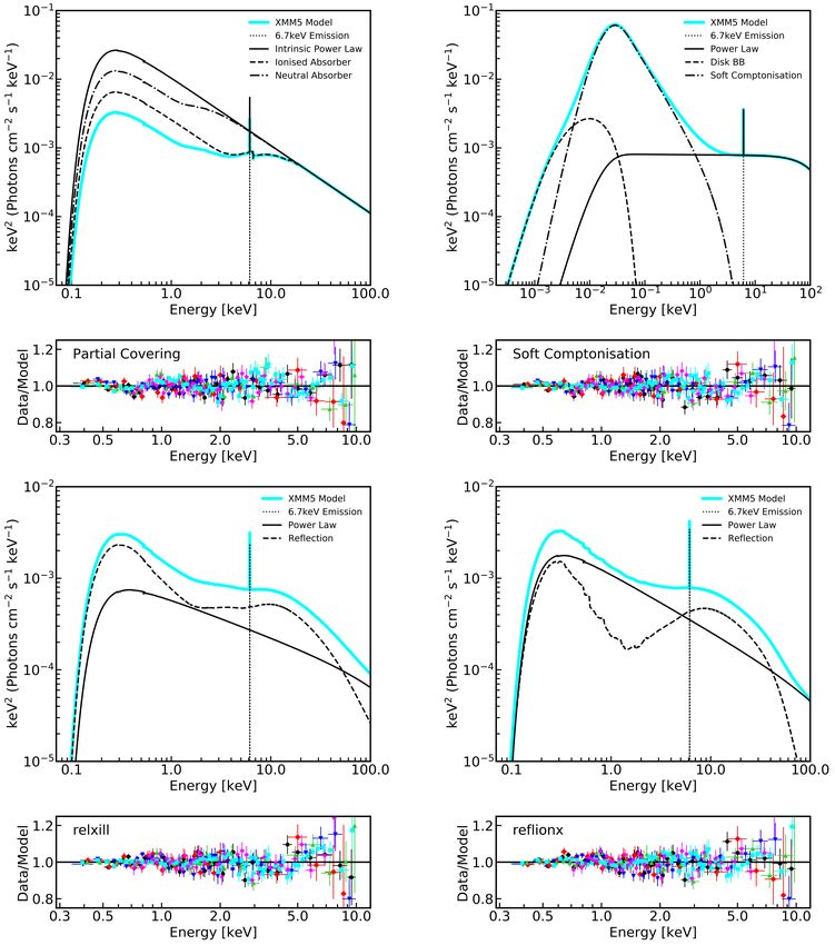
Figure 3. Best-fit model and residuals for physical models in this work. Models are only shown for XMM5 for clarity. Top left: Model components and
residuals for the partial covering scenario. Contributions from the intrinsic power law, ionised absorber, neutral absorber and total model are shown. Residuals
(data/model) are shown in the panel below, displaying significant curvature at high and low energies. Top right: Model components and residuals for the
double Comptonisation model. Effects of Galactic absorption have been removed for clarity, and the axes have been modified accordingly. Contributions
from the disc black body, soft-Comptonisation, and hard Comptonisation are shown. Bottom left: Model components and residuals for the blurred reflection
model using RELXILL. The reflection and power law components are shown, and the intrinsic spectrum is clearly reflection dominated. Bottom right: Model
components and residuals for the blurred reflection model using REFLIONX. The reflection and power law components are again shown, and the resulting
spectrum is not dominated by reflection.
MNRAS 000, 1–15 (2019)Multi-epoch X-ray analysis of Mrk 478 7
the absorption of the brightest spectrum (XMM2) and 5 eV using
the dimmest spectrum (XMM4). No negative residuals are seen,
suggesting that this line strength is consistent with a null detection.
It is also, however, interesting to consider the ionisation on
the other absorber. This value is in agreement with neutral, so this
absorber would also contribute to the Fe Kα line profile. This in-
creases the equivalent width of the line, to 90 eV using the absorp-
tion of the brightest observations, and to 200 eV using the absorp-
tion of the dimmest. Both cases show significant negative residuals
compared to the best-fitting model, implying that these lines should
have been easily detectable in the observed spectrum. This suggests
that non-spherically symmetric absorption is required to produce
the observed spectra.
4.3 Comptonisation
The soft-Comptonisation (e.g. Done et al. 2012) is characterised
by a smooth soft excess as observed in the residuals in Fig. 2. This
model was also suggested to explain the lack of features in the soft
excess observed with the Chandra LETG detector by Marshall et al.
(2003), and for the early XMM-Newton observations by Guainazzi
et al. (2004).
Figure 4. Correlations between best fit parameters using the partial covering To test this physical interpretation, the model OPTXAGNF
model. While no linear trends are observable between data sets, the column (Done et al. 2012) is used. This model describes the X-ray spectrum
density and covering fraction are higher for the dimmer flux XMM4 and above 2 keV with a power law from a hot, spherical corona centred
XMM5 than for other data sets. around the black hole. The soft X-ray spectrum is described with a
second, cooler, optically thick corona located on top of the accre-
tion disc. Emitted power is supplied by the energy released through
free to vary, but kept linked between data sets. This again improves accretion. The mass and accretion rate are fixed at values from Por-
the fit, ∆C = 9 for 2 additional free parameters. No signatures of quet et al. (2004), and the co-moving distance is set to 347 Mpc.
a 6.4 keV emission feature are detected. The best fit energy is at Other free parameters include the radius of the primary, spherical
∼ 6.7 keV, indicating the presence of ionised iron emission as sug- corona (rcor ), the temperature (kT) and opacity (τ) of the soft X-
gested in Section 4.1. ray corona, the slope of the hard Compton power law (Γ), and the
The best fit parameters and MCMC errors for this final model fraction of power emitted in the hard Comptonisation component
are presented in Table 2, and the model and residuals are shown in below rcor (fpl).
the top-left corner of Fig. 3. Parameter correlations for the best fit A variety of combinations of these parameters are tested to at-
model are presented in Fig. 4. The intrinsic power law (shown in tempt to explain the variability between data sets. Allowing only
Fig. 3) is extremely steep, with Γ = 2.99 ± 0.02. The ionisation pa- the soft corona parameters (kT and τ) or only the hard corona pa-
rameter of ZXIPCF is low, poorly constrained, and consistent with rameters (Γ and fpl) to vary did not reproduce the spectral shape,
neutral material. The neutral absorber (ZPCFABS) has a low col- with C = 1045 and C = 1858 for 554 dof respectively. Therefore,
umn density and low covering fraction, and displays only limited all four parameters are left free to vary between epochs. Allowing
variability between epochs. the radius of the primary corona to be free between data sets causes
The ionised absorber displays more significant variability; in it to become unconstrained, so it is linked between epochs. Spin
particular, the covering fraction and density are both higher for the values (a = cJ/GM 2 , where M is the black hole mass and J is
dimmer XMM4 and XMM5 observations, and are lower for the the angular momentum) fixed at 0, 0.5 and 0.998 are tested, with a
brightest data set (XMM2). The higher overall densities and cover- maximum spin giving the best fit.
ing fractions suggest that this component is driving the shape and As with the partial covering model, excess residuals are visible
variability of the observed spectra rather than changes to the intrin- in the 6 − 7 keV band, so a narrow (σ = 1 eV) Gaussian emission
sic power law emission or neutral absorption. line is added. The best fit line energy and normalisation are free
Another aspect of the absorption models is that they do not to vary, but are again linked between epochs. This improves the fit
include the emission lines associated with the included absorption by ∆C = 30 for 2 additional free parameters, for a final fit statistic
edges. The RGS data are consistent with the best-fitting model, but of C = 609 for 546 dof. Again, no signatures of 6.4 keV emission
none of the expected emission lines are present in the RGS spec- are detected - the feature has a best fit energy of 6.6 ± 0.1 keV,
trum. Most notably, the 6.4 keV Fe Kα emission line associated consistent with the line energy found in the partial covering model.
with the edge at ∼ 7 keV is not included in the model. Assuming the The best fit model is shown in the top right panel of Fig. 3,
obscuring sources are spherically symmetric, the predicted strength where the effects of Galactic absorption have been removed for dis-
of the Fe Kα line can be calculated by measuring the absorption play. Best fit parameters are listed in Table 3, and correlations be-
strength of the edge (i.e., the drop in flux in the 7 − 20 keV range), tween parameters are shown in Fig. 5. All parameters appear highly
and multiplying it by the fluorescent yield of iron (e.g. Reynolds correlated with one another, and all change according to the flux of
et al. 2009). If one assumes that only the neutral absorber is re- each spectrum. For the dimmer XMM4 and XMM5, the tempera-
sponsible for producing the 6.4 keV Fe Kα feature, the resulting ture of the secondary corona increases, while the opacity, slope of
emission line is very weak, with an equivalent width of 4 eV using the hard power law, and fpl all decrease compared to the brighter
MNRAS 000, 1–15 (2019)8 S. G. H. Waddell et al.
(1) (2) (3) (4) (5) (6) (7) (8)
Model Parameter XMM1 XMM2 XMM3 XMM4 XMM5 SUZ
Partial Covering (TBABS × CONST × ZPCFABS × ZXIPCF × (ZGAUSS + POWERLAW))
Constant scale factor 1f - 0.96 ± 0.02 - - -
Intrinsic Γ 2.99 ± 0.02 - - - - -
Power Law norm (×10−2 ) 1.1 ± 0.1 - - - - -
Neutral Absorber nH (×1022 cm−2 ) 7±2 3±1 7l 4±1 3.6 ± 0.5 7±2
(ZPCFABS) CF 0.43 ± 0.07 0.36 ± 0.10 0.43l 0.47 ± 0.07 0.50 ± 0.02 0.49 ± 0.06
Ionised Absorber nH (×1022 cm−2 ) 39 ± 12 19 ± 6 39l 43 ± 9 43 ± 7 38 ± 11
(ZXIPCF) log(ξ) (erg cm s−1 ) 0.4 ± 0.5 - - - - -
CF 0.62 ± 0.06 0.65 ± 0.06 0.62l 0.78 ± 0.04 0.75 ± 0.03 0.62 ± 0.06
Ionised Iron E ( keV) 6.7 ± 0.3 - - - - -
Emission σ( eV) 1f - - - - -
Flux (×10−14 erg cm−2 s−1 ) 1.4+1.5
−1.4p
- - - - -
Flux F0.3−10 (×10−11 erg cm−2 s−1 ) 1.23 ± 0.02 1.33 ± 0.03 1.18 ± 0.02 0.72 ± 0.02 0.76 ± 0.01 1.11 ± 0.02
Fit Statistic C/dof 667/544 - - - - -
Table 2. Best fit models for the partial covering scenario, including one neutral and one ionised partial covering component. The model component is given in
column (1), and parameter names are in column (2). Parameters only quoted in the first column are kept linked between data sets. All parameters from XMM3
are linked to those of XMM1, denoted by the superscript "l". All parameters with the superscript "f " are kept fixed at quoted values. Parameters which have
been pegged at a limit are denoted with "p". The normalisation of the power law component is in units of photons keV−1 cm−2 s−1 at 1keV.
(1) (2) (3) (4) (5) (6) (7) (8)
Model Parameter XMM1 XMM2 XMM3 XMM4 XMM5 SUZ
OPTXAGNF ( TBABS × CONST × (ZGAUSS + OPTXAGNF))
Constant scale factor 1f - 0.96 ± 0.02 - - -
Soft-Comptonisation Mass (×107 M ) 1.99 f - - - - -
(OPTXAGNF) Distance (Mpc) 347 f - - - - -
log(Ledd ) −0.027 f - - - - -
a 0.998 f - - - - -
rcor (rg ) 64 ± 5 - - - - -
log(rout ) 3f - - - - -
kT ( keV) 0.26 ± 0.03 0.23 ± 0.02 0.26l 0.6 ± 0.2 0.57 ± 0.12 0.28 ± 0.05
τ 12.1 ± 0.8 13.2 ± 0.8 12.1l 7.2 ± 1.2 7.1 ± 0.8 11.5 ± 1.3
Γ 2.23 ± 0.05 2.18 ± 0.03 2.23l 2.0 ± 0.1 2.01 ± 0.06 2.12 ± 0.05
fpl 0.13 ± 0.01 0.137 ± 0.008 0.13l 0.056 ± 0.005 0.061 ± 0.003 0.100 ± 0.008
Ionised Iron E ( keV) 6.6 ± 0.1 - - - - -
Emission σ( eV) 1f - - - - -
Flux 1.5 ± 0.8 - - - - -
(×10−14 erg cm−2 s−1 )
Flux F0.3−10 1.23 ± 0.04 1.33 ± 0.03 1.18 ± 0.03 0.7 ± 0.3 0.8 ± 0.3 ∼ 1.12
(×10−11 erg cm−2 s−1 )
Fit Statistic C/dof 609/546 - - - - -
Table 3. Best fit models for the soft-Comptonisation model OPTXAGNF. The model component is given in column (1), and parameter names are in column
(2). Parameters only quoted in the first column are kept linked between data sets. All parameters from XMM3 are linked to those of XMM1, denoted by the
superscript "l". All parameters with the superscript "f " are kept fixed at quoted values.
data sets. All parameters are well constrained and vary significantly best fit model to the X-ray data and apply it to optical/UV data, as
between the brighter and dimmer flux epochs. Despite the AGN be- this model is intended for broad SED fitting. To do so, the tool FT-
ing at a bright flux during the SUZ epoch, the parameter values are FLX 2 XSP is used to build dummy response files suitable for use
more intermediate to the high and low states. This could be due to in XSPEC for the available UVW1 and UVW2 data. Only these
the more limited band pass studied with Suzaku. filters are used to avoid potential host galaxy contamination. We
then extrapolate the best-fitting models for both a maximum spin
Another interesting test of the OPTXAGNF model is to take the
MNRAS 000, 1–15 (2019)Multi-epoch X-ray analysis of Mrk 478 9
5 for UVW1 assuming no spin. Allowing the Eddington luminosity
to go free results in a best-fitting super-Eddington accretion rate
(log(L/Ledd )' 0.14) and does not improve the fit to the UV data.
Similarly, simultaneous modelling of the UV and X-ray data fails
to find a fit which explains the UV flux. This shows that the soft-
Comptonisation model is unable to explain the observed SED for
Mrk 478.
4.4 Blurred Reflection
In the blurred reflection model, the intrinsic power law is seen
alongside a reflection spectrum, produced when X-ray photons
from the corona strike the inner accretion disc. This model has been
used successfully to explain the spectral properties and variability
of numerous NLS1 galaxies (e.g. Fabian et al. 2004; Ponti et al.
2010; Gallo et al. 2019b). It has also been used to explain time
domain variability and lags (e.g. Wilkins et al. 2017). This inter-
pretation was also discussed in detail by Zoghbi et al. (2008), who
found that a highly blurred, highly ionised, reflection dominated
model explained the spectra of XMM1 - XMM4.
To test the blurred reflection interpretation, two different mod-
Figure 5. Correlations between best fit parameters using the Comptoni- els are used; RELXILL version 1.2.0 (García et al. 2014) and
sation model. Clear correlations are present between all parameters, and REFLIONX (Ross et al. 1999; Ross & Fabian 2005). REFLIONX
changes between brighter and dimmer flux epochs are evident in all param- was convolved by the blurring model KERRCONV (Brenneman &
eters. Reynolds 2006). REFLIONX was combined with a more simplistic
blurring model KDBLUR for analysis in Zoghbi et al. (2008). Both
of these models are combined with a power law to model the intrin-
sic coronal emission.
To measure the reflection fraction, the convolution model
CFLUX was applied to both the reflection and power law compo-
nents. The flux parameter was linked between the two models. The
relative fluxes of the models were then determined by adding a con-
stant between the reflection and power law components. This con-
stant measures the reflection fraction, R, the ratio of emitted flux in
the reflection and power law components in the 0.1−100 keV band.
Parameters are the same between models. Both include two
emissivity index values qin and qout , separated at a break radius rbr .
These parameters define the illumination pattern, which goes as
∝ r −q . The inner emissivity index is free to vary between epochs,
while the break radius and outer emissivity index are kept fixed
at 6 rg and 3, respectively. The inner radius of the accretion disc
is kept fixed at the innermost stable circular orbit (ISCO), while
Figure 6. All available UVW1 and UVW2 data for all epochs compared the outer radius is fixed at 400 rg , as little emission is expected
to the a = 0 (dashed) and a = 0.998 (solid) best fit Comptonisation models. to originate from outside this radius. The spin (a), inclination and
Colours and shapes match those of the corresponding X-ray data sets. Y-
iron abundance are left free to vary, but linked between epochs, as
axis error bars on the UV data are shown, but are smaller than the symbols.
none are expected to vary within the given timescales. The XSPEC
The best fit models to the X-ray data underestimate the data when extrapo-
lated to UV energies. function STEPPAR is also run on these parameters to ensure that
none are confined to local minima.
The flux produced by the power law component is left free to
(a = 0.998) and non-spinning (a = 0) black hole to the UV data vary between epochs, as is the photon index (Γ). The photon in-
and examine the fit. dex of the reflection component is linked to that of the power law,
The result is shown in Fig. 6. The colours and symbols used as leaving it free to vary does not improve the fit. Various com-
on the optical data match those of the corresponding X-ray spectra. binations between other parameters are tested, and it is found that
No simultaneous optical data is available for the Suzaku data. The the best fit is produced when the reflection fraction and ionisation
best fit models at spins of 0.998 and 0 are shown as black solid and (again defined as ξ = 4πF/n) are left free to vary between observa-
dashed lines, respectively. Models for all data sets are the same at tions, although the changes in these parameters are limited within
this low energy range, so only one model line is shown for each uncertainties between epochs.
spin value. Neither model is able to reproduce the shape or flux of As in the other models, a narrow feature is added to fit the
the data at these low energies. Both underestimate the UV flux, by residuals apparent between 6 − 7 keV. The best fit line energies are
a factor of ∼ 5 for the UVW2 data and ∼ 10 for UVW1, assuming identical for both models, at 6.6 ± 0.1 keV. Once again, no evidence
maximum spin, and a more modest factor of ∼ 3.5 for UVW2 and ∼ for narrow 6.4 keV emission is detected. As such, no distant reflec-
MNRAS 000, 1–15 (2019)10 S. G. H. Waddell et al.
tion model to account for reflection off of the neutral torus is added flection fraction, inner emissivity index and ionisation, but these
to the model. parameters are not well constrained.
The best fit parameters are shown in Table 4, and the mod- The two reflection models presented here (RELXILL and RE -
els and residuals are shown in the bottom two panels of Fig. 3. FLIONX ) are both dominated by a single spectral component in the
Both models produced comparable fits and have the same degrees 0.3 − 10 keV band. For RELXILL, this is the reflection spectrum,
of freedom (539). The C-statistic is 593 and 606 for the RELXILL while REFLIONX suggests the power law dominates. Changes in
and REFLIONX models, respectively. However, each model gives a spectra are caused primarily by flux variations of these compo-
different interpretation of the X-ray emitting region. nents. Both interpretations seem consistent with the approximately
To begin comparing the two models, correlation plots are constant hardness ratio found in Section 3 (see also Section 4.5).
made using the best fitting free parameters. The results are pre-
sented in Fig. 7, with RELXILL parameters shown on the left and
4.5 Principal Component Analysis
REFLIONX parameters shown on the right. Axes between figures
are not identical, but corresponding cells in each panel show cor- To obtain a model-independent assessment of the spectral varia-
relations between the same parameters. The colours and styles of tions between observations, principal component analysis (PCA) is
the data points match those used throughout to represent data sets. used. This technique is implemented using the method and code5
Points for XMM3 are not shown, as these parameters have all been described by Parker et al. (2014). By finding the eigenvalues cor-
linked to XMM1 and are not independently measured. responding to the maximum spectral variability, it allows for the
The inner emissivity is in agreement, although poorly con- detection of correlated variability between energy bands.
strained, between both models for all data sets. For the power law To investigate long-term variability trends, data from all
component, photon indices are generally steeper using REFLIONX XMM-Newton observations are combined and the full 0.3 − 10 keV
than for RELXILL, and do not agree within error. This is also true band is used. The long exposure (XMM5) is broken into seven 20 ks
for the power law fluxes, which are generally higher (brighter) for segments so all spectra have similar exposures. Only one signif-
REFLIONX . For XMM4 and SUZ, however, both of these values icant principal component (PC1) is revealed in this analysis, ac-
agree between models, as these data sets most poorly constrain the counting for ∼ 90 per cent of the variability. This component is
parameters. None of the spectra are as steep as the value measured shown as a function of energy in Fig. 9. The shape is mostly flat,
using partial covering, and are significantly steeper than when us- with some curvature in the 4 − 7 keV region. There is also an up-
ing soft-Comptonisation. turn above ∼ 8.5 keV, which may be attributable to variations in the
background spectrum between epochs. All PC values are positive,
Despite the fact that not all variable parameters agree between
indicating that the changes in each energy band are correlated.
the two reflection models represented here, the parameters kept
Parker et al. (2015) and Gallant et al. (2018) are able to re-
constant between data sets are in agreement with one another; no-
produce this shape with a single variable model component (e.g.
tably black hole spin (a), inclination and iron abundance. This is
a power law) that varies in normalisation. This implies that the
demonstrated in Fig. 8. Data for RELXILL are shown in blue and
spectral changes between epochs can mostly be attributed to flux
data from REFLIONX are in pink. Contours are produced using 68,
changes of a single model component, such as the power law. This
90 and 99 percent of MCMC fits. The histograms reveal that all
interpretation is consistent with the minimal changes in hardness
parameters are evenly distributed around the measured mean. The
ratio within and between observations, and lack of suggested spec-
contours also reveal that all parameters are in agreement, and con-
tral state change based on ∆αox (see Section 3). Significant changes
firm that the reflection interpretation requires a high spin, low in-
in spectral parameters in Mrk 478 are not expected based on the
clination AGN.
PCA. Such changes typically yield more complex principal com-
It is in the interpretation of the reflection fraction and ionisa- ponent shapes, as outlined in Parker et al. (2015). It is important to
tion parameters that the two reflection models are mostly extremely note that more complex physical scenarios, such as multiple vari-
in disagreement. RELXILL suggests a highly ionised spectrum, with able absorption zones, can in some cases produce an overall flat
ξ ' 1000 erg cm−2 s−1 , while REFLIONX predicts a lower value of PCA shape (see Miller et al. 2008), however, the available data are
ξ ' 50 erg cm−2 s−1 . Setting the ionisation parameters of RELX - insufficient to model with more complex scenarios.
ILL to the ones found by REFLIONX and vice versa degrade the fit
PCA also provides a unique way to assess the capability of the
quality by ∆C = 146 and ∆C = 40, respectively. For the reflection models above to reproduce the observed variability. To do so, 100
fraction, use of RELXILL suggests a reflection dominated spectrum, fake data sets with 20 ks exposures are simulated for each model.
with all reflection fractions band constrained to be larger than one, Parameters which are linked between data sets are frozen for all
and the largest being less than 3.5. However, using REFLIONX sug- simulations. Free parameters are varied between each simulated
gests a power law dominated spectrum, or one with equal contri- data set, with ranges based on model constraints. Correlations be-
butions from the intrinsic power law and reflection spectra, with R tween parameters are not apparent using partial covering or RELX -
values constrained between ∼ 0.7 − 1.3 for all spectra. ILL and very weak using REFLIONX , but all parameters are highly
As seen in Fig. 7, using RELXILL suggests that parameters for correlated for OPTXAGNF. A PCA is then produced for these sim-
all data sets are mostly in agreement within error, and no corre- ulated data sets.
lations between parameters are apparent. This is not the case with The results are shown in Fig. 9. The width of the bands rep-
REFLIONX . There is a clear positive correlation between the photon resent the calculated error bars from the PCA analysis. All models
index Γ and the flux of the power law component. This relationship predict correlated variability between all energy bands, but differ
is expected; as Γ increases, more emission is expected in the soft in shape of the first principal component. The PCA results for par-
band, increasing the overall flux. Interestingly, it is also for RE - tial covering and OPTXAGNF exhibit significant curvature, turning
FLIONX that we see clear changes in flux state; with RELXILL , the
flux between epochs does not change within error. For REFLIONX,
weaker evidence for correlations are also visible between the re- 5 http://www-xray.ast.cam.ac.uk/∼mlparker/
MNRAS 000, 1–15 (2019)Multi-epoch X-ray analysis of Mrk 478 11
(1) (2) (3) (4) (5) (6) (7) (8)
Model Parameter XMM1 XMM2 XMM3 XMM4 XMM5 SUZ
REFLIONX ( TBABS × CONST1 × (ZGAUSS + (CFLUX × CUTOFFPL) + (CONST2 × CFLUX × KERRCONV × REFLIONX))
Constant scale factor 1f - 0.89 ± 0.06 - - -
Power Law Γ 2.73 ± 0.06 2.7 ± 0.1 2.73l 2.6 ± 0.1 2.65 ± 0.06 2.8 ± 0.1
Ecut ( keV) 300 f - - - - -
log(F0.1−100 ) −10.67 ± 0.05 −10.66 ± 0.09 −10.67l −11.0 ± 0.1 −10.91 ± 0.04 −10.8 ± 0.1
Blurring Rin (ISCO) 1f - - - - -
(KERRCONV) R ou t (r g ) 400 f - - - - -
R br (r g ) 6f - - - - -
+0.8p +0.6p
qin 8±1 9.0+0.8
−1.4
8l 9.2−1.4 8.9 ± 1.0 9.4−1.2
qout 3f - - - - -
a 0.94 ± 0.02 - - - - -
i (°) < 22 - - - - -
Reflection ξ (erg cm s−1 ) 63 ± 35 55 ± 40 63l < 165 40 ± 22 85 ± 63
(REFLIONX) AFe (Fe/solar) 0.44 ± 0.28 - - - - -
R0.1−100 0.7 ± 0.3 0.8 ± 0.3 0.7l 1.0 ± 0.5 0.7 ± 0.1 1.3 ± 0.6
Ionised Iron E ( keV) 6.6 ± 0.1 - - - - -
Emission σ( keV) 0.001 f - - - - -
Flux (×10−14 erg cm−2 s−1 ) 1.3 ± 0.8 - - - - -
Flux F0.3−10 (×10−11 erg cm−2 s−1 ) 1.23 ± 0.02 1.35 ± 0.03 1.18 ± 0.03 0.7 ± 0.1 0.76 ± 0.02 1.2 ± 0.3
Fit Statistic C/dof 606/539 - - - - -
RELXILL ( TBABS × CONST1 × (ZGAUSS + (CFLUX × CUTOFFPL) + (CONST2 × CFLUX × RELXILL))
Constant scale factor 1f - 0.96 ± 0.02 - - -
Power Law Γ 2.51 ± 0.04 2.47 ± 0.06 2.51l 2.5 ± 0.1 2.42 ± 0.03 2.6 ± 0.2
Ecut ( keV) 300 f - - - - -
log(F0.1−100 ) −11.1 ± 0.2 −11.0 ± 0.1 −11.1l −11.2 ± 0.1 −11.25 ± 0.08 −11.0 ± 0.2
Blurred Rin (ISCO) 1f - - - - -
Reflection Rout (r g ) 400 f - - - - -
(RELXILL) R br (r g ) 6f - - - - -
+1.3p
qin 6.9 ± 0.6 7.3 ± 0.8 6.9l 8.0 ± 1.6 7.8 ± 0.7 8.7−1.8
qout 3f - - - - -
a 0.98 ± 0.01 - - - - -
i (°) 31 ± 8 - - - - -
log(ξ) (erg cm s−1 ) 3.1 ± 0.1 2.8 ± 0.2 3.1l 2.8 ± 0.3 2.9 ± 0.1 2.7 ± 0.4
AFe (Fe/solar) 0.84 ± 0.14 - - - - -
R0.1−100 3.5 ± 1.5 2.3 ± 0.9 3.5l 2.0 ± 0.9 2.4 ± 0.6 3.1 ± 1.7
Ionised Iron E keV 6.6 ± 0.1 - - - - -
Emission σ keV 0.001 f - - - - -
Flux (×10−14 erg cm−2 s−1 ) 1.5 ± 0.8 - - - - -
Flux F0.3−10 (×10−11 erg cm−2 s−1 ) 1.2 ± 0.4 1.33 ± 0.06 1.2 ± 0.4 0.71 ± 0.04 0.8 ± 0.2 1.2 ± 0.1
Fit Statistic C/dof 593/539 - - - - -
Table 4. Best fit models for the blurred reflection models REFLIONX (top) and RELXILL (bottom). Note that const1 refers to the scaling factor between XMM1
and XMM3, while const2 is used to measure the reflection fraction, R. The model component is given in column (1), and parameter names are in column
(2). Parameters only quoted in the first column are kept linked between data sets. All parameters from XMM3 are linked to those of XMM1, denoted by the
superscript "l". All parameters with the superscript "f " are kept fixed at quoted values. Parameters which have been pegged at a limit are denoted with "p".
sharply downwards towards high energies. Both reflection models, in Parker et al. (2015) and Gallant et al. (2018), where normali-
however, produce first principle components which are fairly con- sation changes of a single spectral component produced the PCA
stant across all energies. This is likely due to the fact that most shapes.
variations in these models are in the flux of the dominant emis- To evaluate the statistical fit of each model, χν2 values are ob-
sion component. For RELXILL, this corresponds to flux changes in tained for each simulated PCA compared to the data. For 50 de-
the reflection spectrum, whereas for REFLIONX, this is the power grees of freedom, the χν2 values are 17, 39, 4 and 6 for partial cov-
law component. This is consistent with the simulations presented ering, soft-Comptonisation, RELXILL and REFLIONX, respectively.
MNRAS 000, 1–15 (2019)You can also read