Mitigation of model bias influences on wave data assimilation with multiple assimilation systems using WaveWatch III v5.16 and SWAN v41.20
←
→
Page content transcription
If your browser does not render page correctly, please read the page content below
Geosci. Model Dev., 13, 1035–1054, 2020
https://doi.org/10.5194/gmd-13-1035-2020
© Author(s) 2020. This work is distributed under
the Creative Commons Attribution 4.0 License.

Mitigation of model bias influences on wave data assimilation
with multiple assimilation systems using WaveWatch III
v5.16 and SWAN v41.20
Jiangyu Li1,2 and Shaoqing Zhang1,2,3,4
1 Key  Laboratory of Physical Oceanography, Ministry of Education, Institute for Advanced Ocean Study, Frontiers Science
Center for Deep Ocean Multispheres and Earth System (DOMES), Ocean University of China, Qingdao, 266100, China
2 College of Oceanic and Atmospheric Sciences, Ocean University of China, Qingdao, 266100, China
3 Pilot National Laboratory for Marine Science and Technology (QNLM), Qingdao, 266100, China
4 International Laboratory for High-Resolution Earth System Model and Prediction (iHESP), Qingdao, 266100, China

Correspondence: Shaoqing Zhang (szhang@ouc.edu.cn)

Received: 28 August 2019 – Discussion started: 7 October 2019
Revised: 7 January 2020 – Accepted: 30 January 2020 – Published: 10 March 2020

Abstract. High-quality wave prediction with a numerical           cesses, whether in small-scale coastal simulations or large-
wave model is of societal value. To initialize the wave           scale global climate simulations (e.g., Babanin et al., 2009;
model, wave data assimilation (WDA) is necessary to com-          Huang and Qiao, 2010; Qiao et al., 2004, 2010). The exis-
bine the model and observations. Due to imperfect numerical       tence of ocean waves can modify the structures of both at-
schemes and approximated physical processes, a wave model         mospheric and marine boundary layers by providing sea sur-
is always biased in relation to the real world. In this study,    face roughness, wave-induced bottom stress, breaking-wave-
two assimilation systems are first developed using two nearly     induced mixing and so on, which ultimately influence air–
independent wave models; then, “perfect” and “biased” as-         sea momentum and heat exchange. Therefore, ocean waves
similation frameworks based on the two assimilation systems       are an important component in atmosphere–ocean interaction
are designed to reveal the uncertainties of WDA. A series of      flux processes (e.g., Chen et al., 2007; Doyle, 2002; Liu et al.,
biased assimilation experiments is conducted to systemati-        2011; Warner et al., 2010). In addition, the study of ocean
cally examine the adverse impact of model bias on WDA.            waves can reduce and prevent marine disasters and provide
A statistical approach based on the results from multiple as-     guidance for the development of the social economy (e.g.,
similation systems is explored to carry out bias correction, by   Folley and Whittaker, 2009; Rusu, 2015; Wei et al., 2017).
which the final wave analysis is significantly improved with      Thus, studying ocean waves is of great scientific and social
the merits of individual assimilation systems. The frame-         significance.
work with multiple assimilation systems provides an effec-           At present, ocean wave observational techniques are con-
tive platform to improve wave analyses and predictions and        stantly being improved (e.g., Daniel et al., 2011; Hisaki,
help identify model deficits, thereby improving the model.        2005). Except for traditional buoy observations (e.g., Mit-
                                                                  suyasu et al., 1980; Rapizo et al., 2015; Walsh et al., 1989),
                                                                  satellites can provide much near-real-time wave observa-
                                                                  tional information, which is beneficial for understanding the
1   Introduction                                                  state of ocean waves (e.g., Gommenginger et al., 2003; Lza-
                                                                  guirre et al., 2011; Queffeulou, 2004). However, observations
Ocean waves, referring to the ocean surface gravity waves         always represent scattered samples in time and space in the
driven by wind, are important physical processes in the           real world and therefore do not represent the complete three-
study of multiscale coupled systems. Many studies show            dimensional structure and temporal evolution of real-world
that ocean waves are necessary for upper-ocean mixing pro-        waves.

Published by Copernicus Publications on behalf of the European Geosciences Union.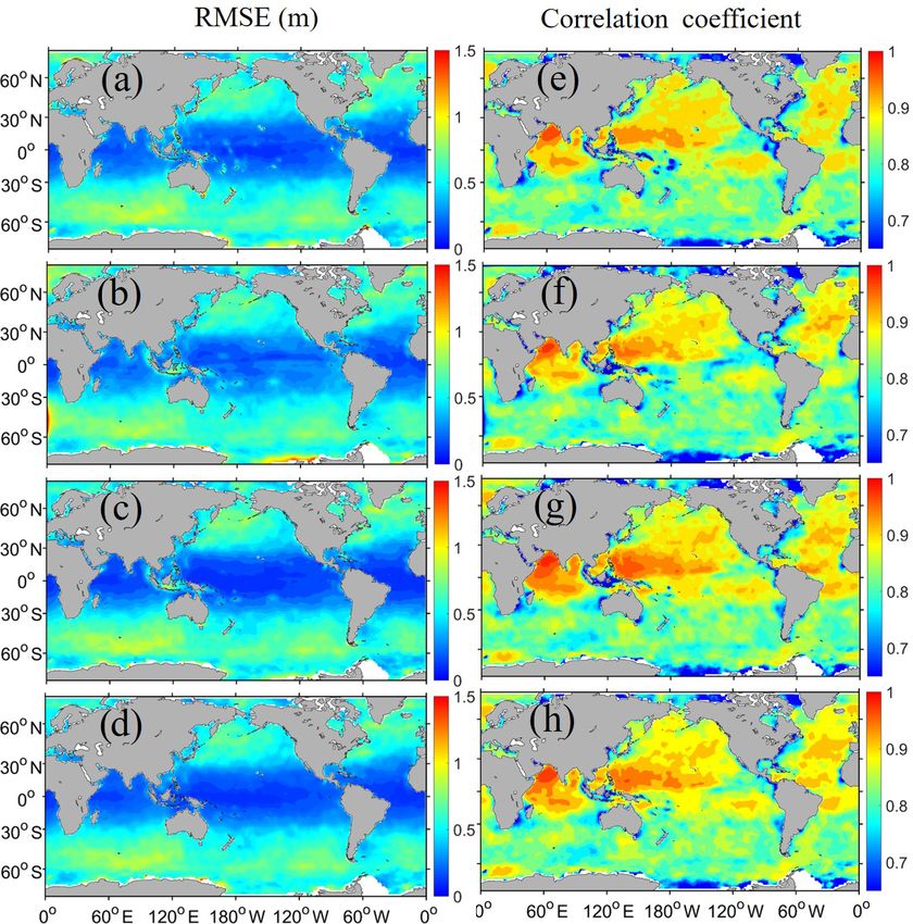
1036                                     J. Li and S. Zhang: Mitigation of model bias influences on wave data assimilation

   Numerical wave models are a powerful tool for study-           use a simple data assimilation scheme with two wave mod-
ing the physical processes of ocean waves and predict-            els (WW3 and SWAN) to explore the influences of different
ing future wave states. Following the development of the          error sources on WDA. The adverse impacts of wind forc-
previous two generations, third-generation wave models,           ing errors and initial-condition uncertainties as well as wave
such as WAve Modeling (WAM) (WAMDI Group, 1988),                  model bias on WDA are studied first, and then two simple
WaveWatch III (WW3) (Tolman, 1991), Simulating Waves              statistical methods for bias correction are developed to miti-
Nearshore (SWAN) (Booij et al., 1999), and MArine Science         gate assimilation errors and improve wave analysis.
and Numerical Modeling (MASNUM) (Yang et al., 2005),                 This paper is organized as follows. After the introduction,
integrate the spectral action balance equation describing the     the methodology is presented in Sect. 2, including a brief
two-dimensional ocean wave spectrum evolution without ad-         description of the employed models and observations, the
ditional ad hoc assumptions regarding the spectral shape, and     development of the two WDA systems using the WW3 and
these third-generation models are more robust for arbitrary       SWAN models, as well as the design of experiments through-
wind fields than previous models. However, there are gener-       out the study. Section 3 presents the model bias analysis and
ally three error sources in wave models. One error source         the adverse impacts of model bias on WDA. In Sect. 4, the
is from an incomplete understanding of the physical pro-          method used to mitigate model bias influences on wave as-
cesses, approximate expressions of the numerical discretiza-      similation is explored. Finally, the discussion and conclusion
tion schemes and so on, which causes systematic errors that       are given in Sect. 5.
are usually referred to as wave model bias. The second error
source is due to inaccurate wind forcings of wave models.
The third error source is from the initial-condition uncertain-   2     Methodology
ties, which can grow due to the nonlinearity of the model
                                                                  2.1     Models and data
equations during model forwarding. In this sense, the model-
simulated waves do not represent the real world either.           2.1.1    Three models
   Given the scattering nature of observational information
and the approximate characteristics of wave modeling, wave        In the wave models, the variance spectrum or energy density
model data assimilation (WDA) is necessary to combine the         E(σ, θ ) is a quantity that represents the wave energy distri-
advantages of both the model and observations. WDA op-            bution in the radian frequency (σ ) and propagation direction
timizes the model initial conditions to produce more accu-        (θ ). Without ambient ocean currents, the variance or energy
rate wave forecasts and produces a more accurate evolution        of a wave package is conserved. However, if the current is
of three-dimensional wave states to elucidate the underly-        involved, due to the work done by the current on the mean
ing mechanisms; this approach dates back to the 1980s (e.g.,      momentum transfer of waves (Longuet-Higgins and Stewart,
Esteva, 1988; Janssen et al., 1989). Since then, many ad-         1961, 1962), the energy of a spectral component is no longer
vanced WDA methods have been developed (e.g., Abdalla             conserved. In general, an action density spectrum defined as
et al., 2013; Bauer et al., 1996; Greenslade and Young, 2004;     N = E/σ is considered within the models. Then, the govern-
Jesus and Cavaleri, 2015; Lionello et al., 1992; Sun et al.,      ing equation of the wave model can be written as follows:
2017; Vorrips et al., 1999), and their applications have been
                                                                  ∂N                  ∂cσ N ∂cθ N   Stot
assessed (e.g., Francis and Stratton, 1990; Heras et al., 1994;      + ∇x · (cg N ) +      +      =      .                    (1)
Stopa and Cheung, 2014). Furthermore, various observation         ∂t                   ∂σ    ∂θ      σ
types, such as buoy, radar and satellite, have been applied       The left-hand side of this equation is the kinematic pro-
to WDA (e.g., Bhatt et al., 2005; Breivik et al., 1998; Feng      cess during wave propagation. The second term describes the
et al., 2006; Greenslade, 2001; Hasselmann et al., 1997; Qi       wave energy propagation in two-dimensional geographical
and Cao, 2016; Voorrips, 1999; Waters et al., 2013), and          space denoted by x. The cg is the group velocity that follows
the wave forecasts have also been directly addressed (e.g.,       the dispersion relation. The third term represents the effect of
Almeida et al., 2016; Emmanouil et al., 2012; Lionello et al.,    shifting the radian frequency due to variation in depth. The
1995; Qi and Fan, 2013; Sannasiraj et al., 2006; Voorrips,        fourth term represents the depth-induced refraction. cσ and
1999; Wang and Yu, 2009; Zhang et al., 2003).                     cθ are wave velocities in the frequency σ and direction θ ,
   Due to the approximate nature of the numerical discretiza-     respectively. On the right-hand side, Stot is the nonconser-
tion and physical processes, a systematic difference between      vative source–sink term representing all physical processes
a model and the real world (i.e., model bias) exists. As noted    that generate, dissipate or redistribute wave energy. Typi-
by Zhang et al. (2012), since model bias is not well defined in   cally, there are three important physical processes that con-
observational space, the influence of model bias on data as-      tribute to Stot , which include the atmosphere–wave interac-
similation is a challenging research topic. Alternatively, one    tion, nonlinear wave–wave interaction and wave–ocean inter-
can simulate model bias using a pair of models and study          action. In a shallow-water case, additional processes must be
the adverse impacts on data assimilation. Inspired by pre-        considered, such as wave–bottom interaction, depth-induced
vious work (e.g., Dee, 2005; Zhang et al., 2012), here, we        breaking and triad wave–wave interaction.

Geosci. Model Dev., 13, 1035–1054, 2020                                             www.geosci-model-dev.net/13/1035/2020/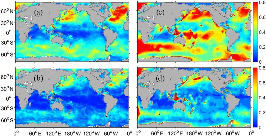
J. Li and S. Zhang: Mitigation of model bias influences on wave data assimilation                                           1037

   In this study, we use three advanced third-generation spec-    2.2   Different modeling strategies in WW3 and SWAN
trum models – WAM (Cycle 4.5.4) (WAMDI Group, 1988),
WaveWatch III (WW3, version 5.16) (Tolman, 1991) and              Since the observations are only a sample of real-world infor-
SWAN (version 41.20) (Booij et al., 1999) – which have im-        mation, the model bias (i.e., systematic difference between
proved a lot from their predecessors, such as numerical and       a numerical wave model and the real world) is not well de-
physical approaches. These wave models have the same form         fined against the real world. In this study, we use the sys-
of governing equation; however their numerical implement          tematic difference between the WW3 and SWAN models to
processes are different due to different considerations. For      simulate the model bias and study the influences on wave
example, SWAN is more focused on wave propagation pro-            data assimilation (WDA).
cesses in shallow water, while WAM and WW3 pay more                  First, let us identity the difference in physical and numeri-
attention to deep water. For more comparisons, please see         cal aspects to comprehend the causes of “bias” between these
Sect. 2.2.                                                        two models. In general, WW3 addresses global scales, and
                                                                  SWAN is more applicable in shallow water. Although the two
2.1.2   Model configurations                                      models have most of the same physical processes, such as the
                                                                  wind input and nonlinear wave–wave interactions, each can
Three wave models use two-dimensional spectral space con-         provide multiple parameterization schemes to choose. For
taining 29 frequencies that cover from 0.035 to 0.555 Hz          example, the nonlinear wave–wave interactions in SWAN in-
with a logarithmic distribution and 24 equidistant direc-         clude the discrete interaction approximation (DIA) (Hassel-
tions. The geographic space is from 180◦ W to 180◦ E in the       mann et al., 1985) and the Webb–Resio–Tracy (Resio and
zonal direction and 75◦ S to 75◦ N in the meridional direc-       Perrie, 1991; Van Vledder, 2006; Webb, 1978), while there
tion with a 1◦ × 1◦ grid resolution. The topography in this       are more choices in WW3, such as the Generalized Multi-
study is taken from the high-resolution ETOPO1 dataset pro-       ple DIA (Toman, 2004, 2013), the two-scale approximation
vided by NOAA (website: https://www.ngdc.noaa.gov/mgg/            and full Boltzmann integral (Perrie et al., 2013; Perrie and
global/, last access: 3 March 2020). The wind forcing has         Resio, 2009; Resio et al., 2011; Resio and Perrie, 2008), as
two sources, both of which have 6 h time intervals. The first     well as the nonlinear filter scheme (Tolman, 2011). In order
dataset is the ERA-Interim reanalysis from the European           to reduce more uncertainties, the same scheme is chosen for
Centre for Medium-Range Weather Forecasts (ECMWF),                the same physical process. In numerical aspects, there exist
with a resolution of 0.75◦ × 0.75◦ (http://apps.ecmwf.int/        different implementation strategies such as the differencing
datasets/data/interim-full-daily/, last access: 3 March 2020).    method, which also contributes to bias.
The second dataset is the CFSRv2 dataset from NCEP, with
a resolution of 0.205◦ (longitude) × 0.204◦ (latitude) (https:    2.3   Two data assimilation systems using WW3 and
//rda.ucar.edu/datasets/ds094.1/, last access: 3 March 2020).           SWAN
The time step of all three models is 15 min. All relevant pa-
rameters above are set to be identical for every wave model       To explore the model bias influences on WDA, we develop
(WW3, SWAN and WAM) in this study.                                two data assimilation systems based on WW3 and SWAN in
                                                                  this study.
2.1.3   Data
                                                                     Generally, based on the program structure of wave mod-
The AVISO (Archiving, Validation and Interpolation of             els, we insert the assimilation module between calculations
Satellite Oceanographic) data (https://www.aviso.altimetry.       of the two-dimensional wave spectrum and outputs of wave
fr/en/data/products/, last access: 3 March 2020) are the satel-   parameters so that at the assimilation time, we call on the as-
lite observational products used in this study. For ocean         similation module to update the spectrum and SWH. When
waves, the AVISO has two satellite altimetry products:            building the data assimilation systems, we need to consider
along-track data and gridded data. The along-track data are       the different structures of parallelism method, data storage
used as the observational data source for the wave data in the    and information exchange in WW3 and SWAN models as
simulation (sampled from “truth” in the “twin” experiments).      noted in Sect. 2.2.
The gridded data are used to validate the wave simulation            To clearly demonstrate the influences of model bias on
and assimilation (1◦ × 1◦ resolution with 1 d time intervals).    WDA and minimize its adverse impact, the analysis scheme
During wave simulation, the significant wave height (SWH)         in both assimilation systems is optimal interpolation (OI),
is used as a basic observational variable for data assimila-      which also is low cost and easy to operate. We implement
tion, which is provided from three ongoing satellites: Jason-     the OI analysis in three to four steps. The first step uses
2, Jason-3, and Satellite for Argos and ALtiKa (SARAL).           two Gaussian convolutions of the background and observed
Figure 1 shows a one-cycle ground orbit by taking Jason-2         SWHs to compute the observational increment of SWH at
and SARAL as examples. Jason-3 is the successor of Jason-         the observational location. The second step projects the SWH
2, and both satellites share the same orbit.                      observational increment onto the model grids centered at the
                                                                  observational location but within an impact radius using lin-

www.geosci-model-dev.net/13/1035/2020/                                              Geosci. Model Dev., 13, 1035–1054, 2020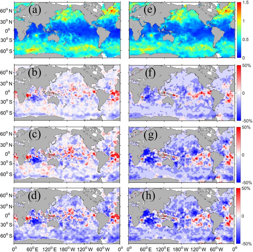
1038                                                 J. Li and S. Zhang: Mitigation of model bias influences on wave data assimilation

Figure 1. The ground projection tracks of satellite Jason-2 (blue line, with an inclination of 66◦ N(S)) and SARAL (red line, with an
inclination of 88◦ N(S)) in one cycle over approximately 10 d and 35 d, respectively, in the (a) global and (b) East Asia domains (zoomed
out of green box in a).

ear regression. The third step transforms the analyzed SWH                   Step 2: regressing the observational increment onto
to update the spectrum of model waves. The fourth step cor-                  model grids
rects wind forcing using the observational SWH.
                                                                             The second step projects the observational increment 1HkO
Step 1: computing observational increment by                                 onto the related model grids using background error co-
convolution of two Gaussians                                                 variance, which is a key step in the analysis. To sim-
                                                                             plify the problem and improve the computational efficiency,
Starting from the idea of the ensemble adjustment Kalman                     many studies use a flow-independent distance function to
filter (Anderson, 2001), an observational increment at the ob-               sample the background error covariance for computing the
servational location k, 1HkO (H represents SWH), is com-                     analysis increment                           A         A
                                                                                         at the model grid i, 1Hi , as 1Hi =
puted by the convolution of two Gaussians of the model                                      d
                                                                             (σis )2 exp − Li,k × 1HkO . Usually, such an expression is
background and observation, which can usually be obtained
from model ensemble members and observational samples.                       only a symmetrical approximation of the correlation function
1HkO is formulated as follows (Zhang et al., 2007):                          and cannot represent the spatial structure and propagation
                                                                             characteristics of waves. Here, with the assumption that wave
            1           M         1       O                                  covariance has the same structure as wave error covariance,
                    H       +           H
          (σ M )2               (σ o )2              1HkM                    we modify the covariance formula to increase its represen-
1HkO =              1             1
                                              +r                M
                                                       M 2 − Hk . (2)
                            +                                                tativeness for wave structure by superimposing a statistical
                (σ M )2         (σ O )2            1 + σσ O                  correlation coefficient obtained from the outputted SWH of
                                                                             model simulation onto the formula. After analysis, the equa-
Here, the first and second terms on the right-hand side of                   tion becomes
the equation adjust the ensemble mean and ensemble spread,                              σis s

                                                                                                       di,k

respectively, and 1HkM represents the prior model spread.
                                                                                   A
                                                                             1Hi = s ri,k exp −                × 1HkO , if di,k ≤ R (3)
                                                                                        σk              L
Superscripts “O” and “M” denote the observation and prior
quantity estimated by the model, respectively. σ is the cor-                 1HiA = 0, if di,k > R,
responding error standard deviation of SWH and varies in                     where L is the characteristic length and di,k is the distance
time and space and differs in every wave model. The overbar                  between the model grid i and observational point k. When
denotes the ensemble mean. In this simplified case, we spec-                 di,k is larger than the impact radius R, there is no observa-
ify σ M = 0.6 m, σ O = 0.25 m, assuming that σ is constant in                tional impact on this model point from observation k. All
all conditions similarly to previous studies (e.g., Qi and Fan,              variables with superscript “s” represent the model statistics
2013), and use single-model and observational values as the                  from free model control results. For example, ri,k     s is the
ensemble mean.                                                               SWH covariance between the model grid i and observation
                                                                             k, which is evaluated from the model data time series in cor-
                                                                             responding experiments. To ensure the local characteristics
                                                                             of ocean waves, in this study, the characteristics length L and
                                                                             impact radius R (or the largest di,k ) are the same, causing this
                                                                             incremental projection to reach to the e-folding scale. Refer-
                                                                             ring to previous studies (e.g., Lionello et al., 1992; Qi and

Geosci. Model Dev., 13, 1035–1054, 2020                                                         www.geosci-model-dev.net/13/1035/2020/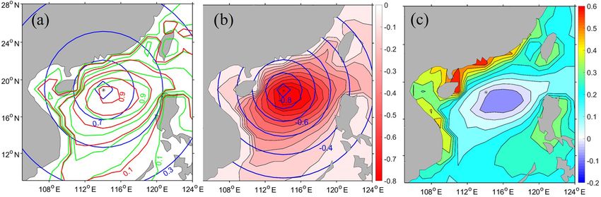
J. Li and S. Zhang: Mitigation of model bias influences on wave data assimilation                                           1039

Fan, 2013), we tested different values of L and R as 300, 800     the along-track observations within a 1 h time window cen-
and 1000 km and found no essential improvement with larger        tered at the time. After 10 d, all the observations will cover
L and R values. Trading-off with computational efficiency,        the global area. The wind data from the reanalysis products
we set L and R to 300 km throughout this study. As shown in       (ERA-Interim and NCEP-CFSR in this case) are available
Fig. 2, the new covariance represents more wave physics; i.e.,    every 6 h. To incorporate the wind correction into the wind
the correlation has more asymmetrical and wave-dependent          forcing of the model, we distribute the wind correction to
characteristics.                                                  the adjacent two time levels of wind data. As the process is
                                                                  looped forward as the wave model state is updated, the wind
Step 3: transforming the SWH to wave spectrum                     forcing is adjusted through the SWH assimilation.

The assimilation SWH HiA is a sum of the prior HiM and the        2.4     Experimental design
analysis increment from step 2 (HiA = HiM + 1HiA ). In the
wave model, the form of ocean waves is a two-dimensional          Throughout this study, we use the symbol MAWF        O(s) as the
wave spectrum that is distributed over frequency and phase.       name for the assimilation experiment. Here, “MA” stands
Thus, transforming the assimilation SWH to a wave spec-           for the “assimilation model” and the subscript “O(s)” (or
trum is necessary to update other wave parameters. Follow-        superscript “WF”) represents the observing system (or wind
ing the previous study (Qi and Fan, 2013), we assume that         forcing) in the assimilation. The wind forcing is either the
the change in wave spectrum is proportional to the energy         ECMWF ERA-Interim (hereafter known as ERAI) or NCEP-
change that is expressed by the square of SWH. Then, the          CFSR wind (hereafter known as CFSR). Wind forcing can
analyzed spectrum SiA (f, θ ) can be written as follows:          also be corrected by observations of SWH (under this cir-
                                                                  cumstance, the superscript “WF” is replaced by “ASSW”).
                      !2
                HiA                                               The observations used in the assimilation could be the model
SiA (f, θ ) =              SiM (f θ ),                     (4)    data but are projected on the along-track points of satellite(s)
                HiM                                               if being used for the twin experiments. Under this circum-
                                                                  stance, “O” represents the “model that produces observa-
where f is the wave frequency and θ is the phase direction.
                                                                  tions” and “(s)” represents the satellite tracks used (J2-Jason-
                                                                  2, J3-Jason-3 and SA-SARAL, for instance). Otherwise, in
Step 4: correcting wind forcing using SWH data
                                                                  the real-data assimilation experiments, the subscript “O(s)”
If the assimilation only adjusts the wave spectrum as de-         directly lists the satellites that measure the SWH. For exam-
scribed in Step 3, the updated spectral structure may be          ple, a symbol named WW3ERAI     SWAN(J2) means that the assim-
quickly overwritten by erroneous wind. In this step, we de-       ilation model is WW3 (here, “MA” = “WW3”) forced by
scribe a simple scheme using the observed SWH data to cor-        ERA-Interim wind (“WF” = “ERAI”), and the model pro-
rect the wind forcing. Starting from a first guess of wind (the   ducing observation is SWAN with the Jason-2 satellite track
ERA-Interim reanalysis, for instance), the analyzed wind          (“O” = “SWAN” and “(s)” = “(J2)”).
   A at model grid (i, j ) can be written as follows:
Wi,j
                                                                  2.4.1    Twin experiments
  A      M
Wi,j = Wi,j + 1Wi,j ,                                      (5)    Twin experiments refer to a type of observing system simula-
                                                                  tion experiment (OSSE), in which a model simulation is used
where W represents either the u or the v component of wind.       to define the “true” solution of a data assimilation problem
1Wi,j is the corrected wind increment transformed from            and the other model simulation is used to start the assimila-
the updated SWH. While the details of the transformation          tion. The “observations” are samples of the truth with some
scheme can be found in Lionello et al. (1992, 1995), we com-      white noise to simulate the observational errors. When the
ment on certain aspects relevant to our study. Regardless of      truth and assimilation are conducted by different (or identi-
boundaries, in general, the energy of ocean waves is deter-       cal) models, the framework is a “biased” (or “perfect”) model
mined by the wind speed and duration, which can also be           twin experiment. Within a twin experiment framework, any
expressed by SWH. In that sense, a function equation can be       aspect of assimilation skills can be measured as the degree to
built, in which the left-hand side is an expression of wind       which the truth is recovered through the assimilation.
speed and duration, while the right-hand side is an expres-
sion of SWH, and they are balanced through wave energy.           (a) Perfect twin experiment
Then, the analyzed wind speed can be resolved under the as-
sumption that the duration is the same in both the prior and      In a perfect twin experiment, we assume that the assimilation
the analyzed fields.                                              model and the observation are unbiased; i.e., both the instru-
   With respect to the configuration of wave model data as-       ment measuring and numerical modeling processes are sam-
similation, the model time step is 15 min and the assimila-       pling the same stochastic dynamical system. Such sampling
tion interval is 1 h. At the assimilation time, we assimilate     only has random sampling errors without any systematic dif-

www.geosci-model-dev.net/13/1035/2020/                                              Geosci. Model Dev., 13, 1035–1054, 2020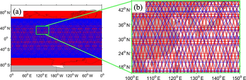
1040                                       J. Li and S. Zhang: Mitigation of model bias influences on wave data assimilation

Figure 2. Spatial distributions of (a) background correlation coefficients by the empirical correlation model (blue), model data statistics
(green) as well as their combination (red) of Eq. (3), (b) background adjustment increments of SWH projected from the observational
increment with the empirical correction model (blue line) and their combination model (red filled), and (c) the difference in background
adjustment increments of SWH from (b) by an analysis process given the single observation obtained at 18.90◦ N, 114.09◦ E, denoted by the
asterisk (unit: m).

ference (bias). We can build this perfect model framework by               Under the biased twin experiment framework, we also
using the same model to produce the truth as the assimilation           conduct experiments to examine the impacts of ob-
model but with different initial conditions and wind forcings.          serving systems on wave assimilations by increasing
   The observations from the observational time window                  the observational information based on multiple satel-
(1 h) centered at the assimilating time can be created by sam-          lite tracks. For example, we can examine the assim-
pling the truth SWH with the tracks of Jason-2, Jason-3 and             ilation results of WW3WF                   WF
                                                                                                  SWAN(J2) , WW3SWAN(J2+J3) and
SARAL, which will cover the global area in 10 d. In this cir-           WW3SWAN(J2+J3+SA) (or SWANWW3(J2) , SWANWF
                                                                               WF                        WF
                                                                                                                         WW3(J2+J3)
cumstance, if WW3 (or SWAN) is used as the assimilation                 and SWANWF                ) to understand the impacts of ob-
                                                                                    WW3(J2+J3+SA)
model, the truth is produced by the same WW3 (or SWAN)                  serving systems on different model-based assimilations.
model. In the assimilation, we may start the model with dif-
ferent initial conditions and/or wind forcings to examine the           2.4.2    Real-data assimilation experiments
influences of initial errors and wind forcing errors on the
wave assimilation. Such a perfect twin experiment can be                In this study, we also conduct real-data assimilation experi-
named WW3WF                     WF
               WW3(s) or SWANSWAN(s) .                                  ments using WW3 and SWAN assimilation systems with real
                                                                        track data from Jason-2, Jason-3 and SARAL. Through real-
(b) Biased twin experiment                                              data assimilation experiments with different model-based as-
                                                                        similation systems, we can (1) increase our understanding of
To study the impact of model errors on wave assimilation, we            the influences of model errors on the WDA and (2) study the
use two models to design a biased twin experiment. Again,               method to reduce the model error influences on the assimi-
due to the scattering nature of the observations, it is difficult       lation results. The real-data assimilation experiments can be
to obtain a complete picture of the model bias against the real         directly named, i.e., WW3WF                    WF
                                                                                                    J2+J3+SA or SWANJ2+J3+SA .
world. Given the difference between the WW3 and SWAN
models described in Sect. 2.2, we use these two models and
their assimilation systems here to simulate the model bias              3     Error sources in wave models and WDA
and examine its influences on the WDA. We use the ERA-
Interim reanalysis wind to force the WW3 (or SWAN) to                   3.1     Influences of initial and wind forcing errors
produce the truth and observations but use the SWAN (or
WW3) assimilation system to assimilate the observations.                Usually, wave numerical simulation can be improved by
The degree to which the truth produced by different model-              three methods: (1) reducing the errors in the initial condi-
based assimilation systems is recovered by assimilating the             tions, (2) enhancing the accuracy of the wind forcing, and
observations is an assessment of the model bias influences              (3) improving the representation of the wave model and its
on the WDA. Such a biased twin experiment can be named                  parameterization.
WW3WF                    WF                                                In this section, we use perfect model twin experiments
      SWAN(s) or SWANWW3(s) .
                                                                        (as described in Sect. 2.4.1) to exclude model errors and
                                                                        explore the impact of wind forcings and initial conditions

Geosci. Model Dev., 13, 1035–1054, 2020                                                    www.geosci-model-dev.net/13/1035/2020/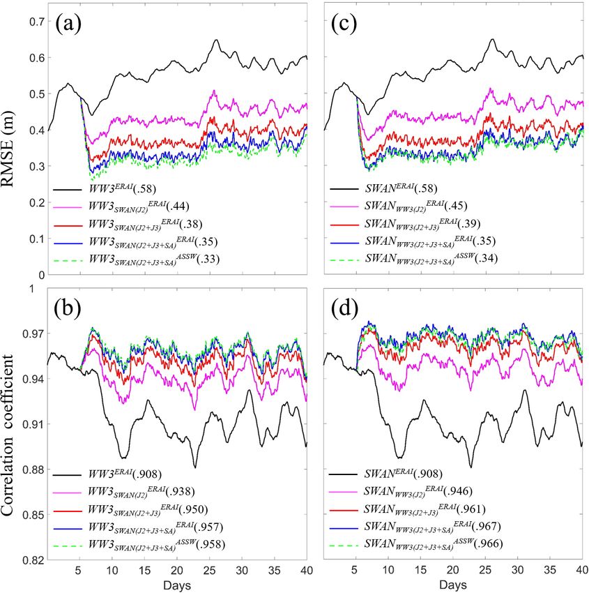
J. Li and S. Zhang: Mitigation of model bias influences on wave data assimilation                                                  1041

Table 1. List of perfect model twin experiments.

  Exp. name                  Model      Wind force    Assimilation or not                         Role
  WW3ERAI                    WW3        ERA-Interim   No                                          Truth for WW3 assimilation
  WW3CFSR                    WW3        NCEP-CFSR     No                                          Model control for WW3 assimila-
                                                                                                  tion reference
  WW3CFSR
     WW3(J2)                 WW3        NCEP-CFSR     Yes (using Jason-2 track)                   Impact of observational system
  WW3CFSR
     WW3(J2+J3)              WW3        NCEP-CFSR     Yes (using tracks of Jason-2 and Jason-3)
  WW3CFSR
     WW3(J2+J3+SA)           WW3        NCEP-CFSR     Yes (using tracks of Jason-2, Jason-3 and
                                                      SARAL)
  SWANERAI                   SWAN       ERA-Interim   No                                          Truth for SWAN assimilation
  SWANCFSR                   SWAN       NCEP-CFSR     No                                          Model control for SWAN assimila-
                                                                                                  tion reference
  SWANCFSR
      SWAN(J2)               SWAN       NCEP-CFSR     Yes (using Jason-2 track)                   Impact of observational system
  SWANCFSR
      SWAN(J2+J3)            SWAN       NCEP-CFSR     Yes (using tracks of Jason-2 and Jason-3)
  SWANCFSR
      SWAN(J2+J3+SA)         SWAN       NCEP-CFSR     Yes (using tracks of Jason-2, Jason-3 and
                                                      SARAL)

on the wave simulations. To compare the performances of              and SWANCFSR + SWANERAI ) and pink (for WW3CFSR +
the WW3 and SWAN models, we conduct separate exper-                  WW3ERAIWW3(J2) and SWAN
                                                                                               CFSR
                                                                                                    + SWANERAISWAN(J2) ) lines.
iments with these two models. The truth and model control               The SWH RMSE is approximately 0.34 m in the WW3
runs are two basic experiments of the perfect twin experiment        or SWAN model control with the NCEP-CFSR wind. Once
framework. We use the ERA-Interim wind to drive WW3 (or              the wind forcing is changed to the perfect wind (the ERA-
SWAN) and generate a long time series of model states as             Interim) on the 45th day, the RMSE quickly drops and is
the “truth,” which is called WW3ERAI (or SWANERAI ) for the          close to zero after approximately 10 d, and the SWAN model
WW3 (or SWAN) perfect model twin experiment. The obser-              takes longer to accomplish this change than the WW3. If
vations are created by interpolating the corresponding truth         data assimilation is added, the RMSE reduces much faster
SWH onto the along-track points of satellite orbits. Then,           than the model controls (roughly half of the timescale of the
we use the NCEP-CFSR wind to force WW3 (or SWAN),                    correct wind forcing). From the analyses above, we learned
called the model control WW3CFSR (or SWANCFSR ), and the             (1) in wave models, the wind forcing plays an important role
data assimilation is named WW3CFSR                     CFSR
                                   WW3(s) (or SWANSWAN(s) ).         and an incorrect wind forcing could be a significant error
Starting from an independent initial condition produced by           source of WDA, and (2) the WDA can rapidly reduce the
the model control, we can conduct the assimilation with the          initial error and improve the predictability of a wave model
ERA-Interim or NCEP-CFSR wind forcing. The error verifi-             even when it is forced by an inaccurate wind forcing.
cation of the assimilation results against the truth simulation
compared to the error of the model control is an evaluation          3.2    Impact of the observational system
of the initial error and/or wind forcing error influences on
the WDA. All perfect model twin experiments are listed in            In this section, using the same model states (at the
Table 1.                                                             45th day) in the corresponding model control as
   First, we conduct two sets of model control experiments           in Sect. 3.1 as the initial conditions, we conduct
WW3CFSR and SWANCFSR for 80 d (from December 2017                    two sets of assimilation experiments: WW3CFSR        WW3(J2) ,
to February 2018). To explore the effect of the initial con-               CFSR              CFSR                        CFSR
                                                                     WW3WW3(J2+J3) , WW3WW3(J2+J3+SA) and SWANSWAN(J2) ,
ditions, we perform the model spin-up for a long time to
adequately reach a steady state. Then using the 45th-day             SWANCFSR                   CFSR
                                                                            SWAN(J2+J3) , SWANSWAN(J2+J3+SA) . Through exam-
model states as the initial conditions, we conduct one more          ining the assimilation quality with one satellite (Jason-2),
model simulation and data assimilation experiments for each          two satellites (Jason-2+Jason-3) and three satellites (Jason-
model system as WW3ERAI and WW3ERAI                                  2+Jason-3+SARAL), we attempt to understand the impact
                                           WW3(J2) as well as
        ERAI              ERAI                                       of improving the observing system on the WDA, considering
SWAN          and SWANSWAN(J2) . The root mean square er-
                                                                     the NCEP-CFSR wind forcing errors against the ECMWF
rors (RMSEs) of these experiments against the truth are
                                                                     ERA-Interim based on a perfect assimilation model. The
shown in Fig. 3 as the red (for WW3CFSR + WW3ERAI
                                                                     RMSEs of all the above assimilation experiments are plotted

www.geosci-model-dev.net/13/1035/2020/                                                  Geosci. Model Dev., 13, 1035–1054, 2020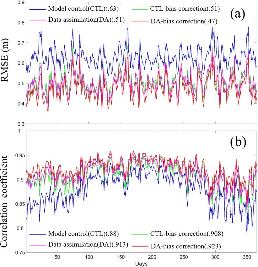
1042                                       J. Li and S. Zhang: Mitigation of model bias influences on wave data assimilation

Figure 3. The time series of RMSEs of the (a) WW3 and (b) SWAN perfect model experiments in the model control run with the NCEP
CFSRv2 wind (black, denoted as WW3CFSR in panel (a) and SWANCFSR in (b), assimilating the “observed” data sampled by the tracks of
Jason-2 (blue, denoted as WW3CFSR              CFSR                                           CFSR                 CFSR
                              WW3(J2) and SWANSWAN(J2) ), Jason-2 and 3 (green, denoted as WW3WW3(J2+J3) and SWANSWAN(J2+J3) ),
as well as Jason-2 and 3 and SARAL (cyan, denoted as WW3CFSR                                 CFSR
                                                                WW3(J2+J3+SA) and SWANSWAN(J2+J3+SA) ) against the truth simulation
forced by the ERA-Interim wind. The red and pink are forced by the NCEP CFSRv2 wind in the first 45 d, but the next 35 d are forced
using the ERA-Interim wind (same as truth) without (denoted as WW3CFSR + WW3ERAI and SWANCFSR + SWANERAI ) or with (denoted
as WW3CFSR + WW3ERAI   WW3(J2) and SWAN
                                          CFSR + SWANERAI
                                                          SWAN(J2) ) the assimilation of Jason-2 data. The number in parentheses for each
color is the corresponding RMSE averaged globally over the verification time period (30 d after the 45 d model spin-up and 5 d assimilation
spin-up). The observed data are produced by projecting the truth SWH onto the satellite orbit.

in Fig. 3 as the blue (assimilating Jason-2 only), green                verse impact of the model bias on the wave assimilation, the
(assimilating Jason-2+Jason-3) and cyan (assimilating                   biased twin experiments described in Sect. 2.4.1 are used
Jason-2+Jason-3+SARAL) lines.                                           in this section, where the truth model and the assimilation
   From Fig. 3, we can see that in both models, the assimi-             model are different between WW3 and SWAN. For exam-
lation errors are reduced when more observational informa-              ple, the WW3ERAI                      ERAI
                                                                                       SWAN(J2) (or SWANWW3(J2) ) experiment uses
tion is used. The corresponding RMSE reductions in these                WW3 (or SWAN) as the assimilation model to assimilate the
three experiments from the model control run are 24 %, 32 %             Jason-2 track point observations, but the observed values are
and 38 % for WW3 and 26 %, 35 % and 38 % for SWAN,                      produced by SWAN (or WW3), and all models are forced by
respectively. However, when more satellite observations are             the ERA-Interim wind. All related experiments for the biased
assimilated into the model, the magnitude of improvement                model framework are described in detail in Table 2.
becomes small (further reduced by 8 % in WW3 and 9 % in                    The RMSEs and correlation coefficients produced by the
SWAN when Jason-3 is added as well as only a 6 % in WW3                 all biased model assimilation experiments are plotted in
and 3 % in SWAN further reduction when SARAL is further                 Fig. 4. The black line in each panel represents the result of
added). These results suggest that given wind forcing errors,           the WW3 model control forced by the ERA-Interim wind
increasing observational information can help to improve the            (WW3ERAI ) against the truth simulation by the SWAN model
model behavior, but the improvement is limited.                         with the same wind forcing (SWANERAI ) (panels a and b)
                                                                        (vice versa in panels c and d). Both the WW3ERAI and
3.3    Adverse impact of model bias                                     SWANERAI experiments are initialized from a cold start by
                                                                        the wind and integrated for 80 d, and the results of the last
                                                                        40 d are shown in Fig. 4. It is clear that the WW3 and SWAN
As described in Sect. 2.2, the WW3 and SWAN models
                                                                        model simulations are quite different even though both sim-
discretize the wave-action-governing equation with different
                                                                        ulations use identical forcings and start from identical ini-
physical processes, parameterization schemes and differenc-
                                                                        tial conditions. The RMSEs of the two model simulations
ing schemes. These differences result in each wave model
                                                                        are both 0.58 m, which is much larger than the errors pro-
having its own distinguished characteristics. To study the ad-

Geosci. Model Dev., 13, 1035–1054, 2020                                                    www.geosci-model-dev.net/13/1035/2020/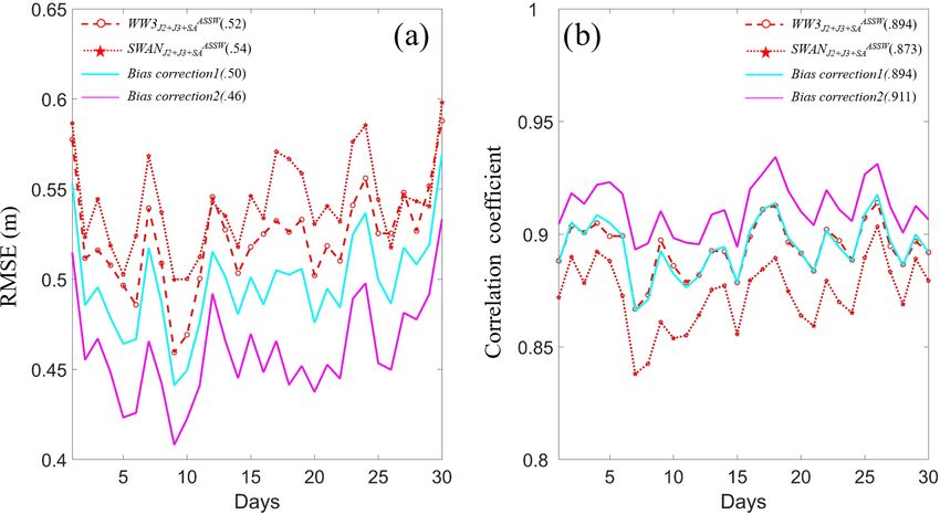
J. Li and S. Zhang: Mitigation of model bias influences on wave data assimilation                                                1043

Table 2. List of biased model twin experiments.

 Exp. name                 Model      Wind source              Assimilation or not                 Role
 WW3ERAI                   WW3        ERA-Interim              No                                  Truth for SWAN assimilation
 SWANERAI                  SWAN       ERA-Interim              No                                  Model control for SWAN assimila-
                                                                                                   tion reference
 SWANERAI
     WW3(J2)               SWAN       ERA-Interim              Yes (using Jason-2 track)           Impact of observational system
 SWANERAI
     WW3(J2+J3)            SWAN       ERA-Interim              Yes (using tracks of Jason-2 and
                                                               Jason-3)
 SWANERAI
     WW3(J2+J3+SA)         SWAN       ERA-Interim              Yes (using tracks of Jason-2,
                                                               Jason-3 and SARAL)
 SWANASSW
     WW3(J2+J3+SA)         SWAN       Assimilation-corrected   Yes (using tracks of Jason-2,       Impact of assimilation-corrected
                                      wind based on ERAI       Jason-3 and SARAL)                  wind
 SWANERAI                  SWAN       ERA-Interim              No                                  Truth for WW3 assimilation
 WW3ERAI                   WW3        ERA-Interim              No                                  Model control for WW3 assimila-
                                                                                                   tion reference
 WW3ERAI
    SWAN(J2)               WW3        ERA-Interim              Yes (using Jason-2 track)           Impact of observational system
 WW3ERAI
    SWAN(J2+J3)            WW3        ERA-Interim              Yes (using tracks of Jason-2 and
                                                               Jason-3)
 WW3ERAI
    SWAN(J2+J3+SA)         WW3        ERA-Interim              Yes (using tracks of Jason-2,
                                                               Jason-3 and SARAL)
 WW3ASSW
    SWAN(J2+J3+SA)         WW3        Assimilation-corrected   Yes (using tracks of Jason-2,       Impact of assimilation-corrected
                                      wind based on ERAI       Jason-3 and SARAL)                  wind

duced by a perfect model but with different wind (∼ 0.34 m,          “corrected” by the “observed” SWH data, as described in
see black lines in Fig. 3).                                          Step 4 of Sect. 2.3. We found that in both assimilation sys-
   Compared with the model controls WW3ERAI and                      tems, using the observed SWH data to “correct” the wind
SWANERAI , the assimilation experiments WW3ERAI SWAN(J2) and         can compensate for the model errors to some degree and fur-
        ERAI
SWANWW3(J2) (pink lines in Fig. 4) can significantly re-             ther reduce the assimilation errors, but the improvement is
duce the SWH simulation error (by 24 % and 22 %, respec-             very limited. The weak improvement could be attributed to
tively) and enhance the correlations (by 3 % and 4 %, re-            the simple wind correction method with total wave height. In
spectively) with the truth (SWANERAI and WW3ERAI , re-               the future, a more powerful correction method with wind sea
spectively). When the observations of Jason-3 and SARAL              wave height may have better performance.
are added to the assimilation (i.e., WW3ERAI                            These assimilation results clearly show that even though
                                             SWAN(J2+J3) and
                                                                     the wind forcing is perfect, once a biased assimilation model
WW3ERAISWAN(J2+J3+SA)    as well  as  SWAN   ERAI
                                             WW3(J2+J3) and
        ERAI
                                                                     is used, the wave simulation has large errors. Although WDA
SWANWW3(J2+J3+SA) ) (see the red and blue lines, respec-             can greatly reduce the simulation error by assimilating the
tively), the model SWH error (or correlation) is further re-         observational information into the model, due to the exis-
duced (or enhanced), but the amplitude of reduction (or en-          tence of the model bias, the error remains at some significant
hancement) gradually diminishes (10 % and 5 % for further            level and cannot be eliminated entirely even by increasing
error reduction and 1 % and 0.8 % for further correlation en-        the observational constraints through an improvement in the
hancement in the WW3 assimilation; 10 % and 7 % for fur-             observational system and constraint of the wind forcing.
ther error reduction and 1.7 % and 0.7 % for further correla-
tion enhancement in SWAN assimilation from the additions
of Jason-3 and SARAL, respectively).                                 3.4    Comparison of the influence of wind forcing with
   The results of two other sets of assimilation experiments                model bias
called WW3ASSW                            ASSW
              SWAN(J2+J3+SA) and SWANWW3(J2+J3+SA) are
also plotted by dotted green lines in Fig. 4. The superscript        Comparing the time series of SWH RMSE caused by two im-
“ASSW” stands for the assimilation-corrected wind, mean-             portant error sources, model bias (0.58 m shown with black
ing that the wind forcing of the assimilation model is also          lines in panels a and c in Fig. 4) plays a stronger role than
                                                                     wind forcing (0.34 m shown with black lines in Fig. 3). When

www.geosci-model-dev.net/13/1035/2020/                                                   Geosci. Model Dev., 13, 1035–1054, 2020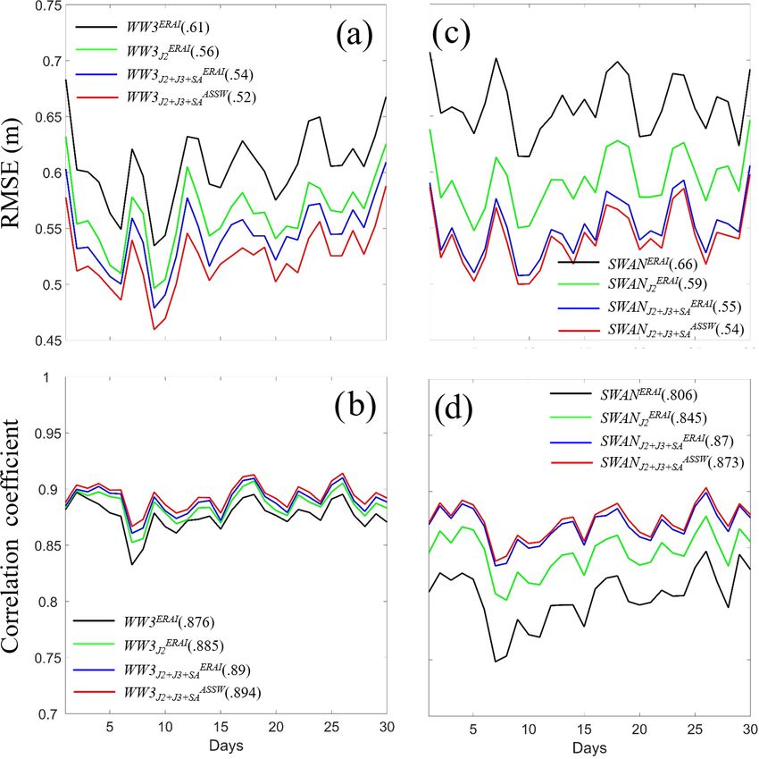
1044 J. Li and S. Zhang: Mitigation of model bias influences on wave data assimilation
Figure 4. The time series of RMSEs (a, c) and spatial correlation coefficients (b, d) of the WW3 (a, b) and SWAN (c, d) biased
model experiments in the model control run forced by the ERA-Interim wind (black, denoted as WW3ERAI and SWANERAI ), assimila-
tions with “observed” data from one (pink, denoted as WW3ERAI ERAI ERAI
SWAN(J2) and SWANWW3(J2) ), two (red, denoted as WW3SWAN(J2+J3) and
SWANERAI ERAI ERAI
WW3(J2+J3) ) and three (blue, denoted as WW3SWAN(J2+J3+SA) and SWANWW3(J2+J3+SA) ) satellites, as well as the assimilation
with corrected wind (dotted green, denoted as WW3ASSW ASSW
SWAN(J2+J3+SA) and SWANWW3(J2+J3+SA) ) against the truth (same as in Fig. 3 but
for SWAN and WW3 with the ERA-Interim wind). The numbers in the parentheses correspond to the globally averaged RMSE (in a and c)
and spatial correlation coefficient (in b and d) over the last 30 d during the assimilation period. The observed data are produced by projecting
the truth SWH onto the satellite orbit.
three satellite observations (Jason-2, Jason-3 and SARAL) as simulation/assimilation model.) In the model control run,
are assimilated into twin experiments, the RMSE of SWH re- it makes sense that the error caused by wind forcing (panel
duces by 38 % in perfect model twin experiments (cyan lines a (WW3CFSR ); truth is WW3ERAI ) has distributed in the ar-
in Fig. 3) and 40 % in biased model twin experiments (blue eas where the wind is strong, such as the area of the Antarctic
lines of panels a and c in Fig. 4). It is obvious that the error Circumpolar Current (ACC) and the north Pacific and At-
caused by model bias is bigger than by wind forcing and their lantic Ocean, while the error caused by model bias (panel c
improvements are almost similar after data assimilation. (WW3ERAI ); truth is SWANERAI ) is distributed almost glob-
A spatial pattern of SWH RMSE is also displayed in ally. After assimilating with three satellite observations, the
Fig. 5. (Due to the similar performance inside twin exper- error spatial distribution of both has improved a lot (panel b
iments, here we only show the results using WW3 model (WW3CFSR ERAI
WW3(J2+J3+SA) ) and panel d (WW3SWAN(J2+J3+SA) )).
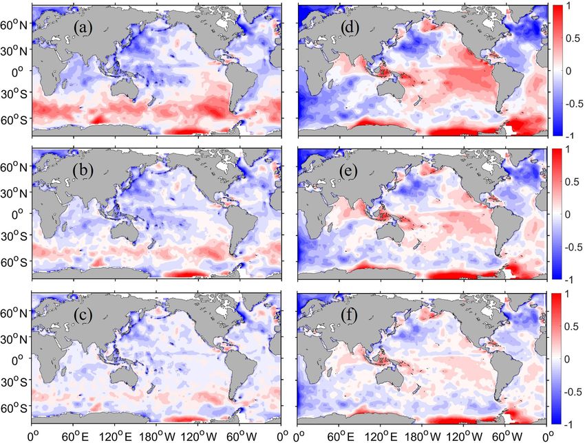
Geosci. Model Dev., 13, 1035–1054, 2020 www.geosci-model-dev.net/13/1035/2020/J. Li and S. Zhang: Mitigation of model bias influences on wave data assimilation 1045
Figure 5. Distributions of SWH RMSEs caused by wind forcing (a, b) from perfect twin experiment and model bias (c, d) from biased twin
experiment in the model control run (a, c) and assimilations with “observed” data with three satellites (b, d) averaged globally over the last
30 d during the assimilation period.
Referring to wind distribution, we can divide the global areas forcing have errors, we will analyze and discuss how to mit-
roughly into three parts: the northern westerly zone (65◦ N– igate the model bias influences on the WDA.
30◦ N), the trade-wind zone (30◦ N–30◦ S) and the circumpo-
lar westerly zone (30◦ S–65◦ S). Therefore the error is caused
by wind forcing (or model bias); the decreasing percentages 4 Mitigation of model bias influences on wave
of SWH RMSE in these three areas are 30 % (or 27 %), 45 % assimilation
(or 50 %) and 46 % (or 48 %), respectively. We can find that
the improvement of both error sources has a similar perfor- 4.1 Bias characteristics of WW3 and SWAN data
mance in three these areas: weak in the northern westerly assimilations
zone and almost the same strength in the trade-wind zone and
circumpolar westerly zone. The reason why there is a lower From the above analyses of twin experiment results, we
improvement in the north Pacific and Atlantic Ocean should learned that the model bias has a strong adverse impact on
be explored in the future. To sum up, the error caused by WDA. To explore the method of mitigating the model bias
model bias is larger than wind forcing in the global area gen- influence on the WDA, we conduct the real-data assimila-
erally, especially in the equatorial ocean. However, in the tion experiments (same time range as the twin experiments)
north of Atlantic Ocean, wind forcing has a stronger im- described in Sect. 2.4.2 using the WW3 and SWAN assim-
pact. After data assimilation, both have improved greatly and ilation systems to assimilate the track data of Jason-2 and
have a similar spatial pattern (i.e., the bigger error is still dis- Jason-2+Jason-3+SARAL. To ensure the performance of
tributed at high latitudes). However, their error gap still ex- the biased model WDA, a longer assimilation (more than 2
ists. months) is conducted (a total of 70 d). The spatial distribu-
It is worth mentioning that there is a similar performance tions of the SWH errors (obtained from the difference against
about the effect of the observation system on improving both the merged gridded AVISO observations over the last 30 d
error sources, whether in time series or spatial distribution. out of 80 d) are shown in Fig. 6. Panels a, b and c (d, e,
The more observation information is absorbed into assimila- f) are for the WW3 (SWAN) simulation and assimilations:
tion systems, the better the error improvement in both twin WW3ERAI , WW3ERAI J2 and WW3ERAIJ2+J3+SA (or SWAN
ERAI ,
experiments. However, due to the existence of model bias, ERAI ERAI
SWANJ2 and SWANJ2+J3+SA ).
this improvement has a limitation and stays at a certain level. Comparing panel a with panel d in Fig. 6 reveals that
If more powerful observation is absorbed (such as wave di- a large difference exists in the simulations of the two models.
rection, wave period and two-dimensional wave spectra), the First, the SWAN simulation errors are generally larger than
limitation maybe stay at a lower level. Next, with the re- the WW3 simulation errors. Second, the global error distri-
sults of real-data assimilation where both the model and wind butions are quite different: while the WW3 simulation errors
www.geosci-model-dev.net/13/1035/2020/ Geosci. Model Dev., 13, 1035–1054, 20201046 J. Li and S. Zhang: Mitigation of model bias influences on wave data assimilation Figure 6. Distributions of SWH mean errors (against the merged grid altimeter data) of the WW3 (a–c) and SWAN (d–f) model simula- tions (a, d) and assimilations with Jason-2 (b, e), as well as all Jason-2, Jason-3 and SARAL (c, f) data forced by the ERA-Interim wind. The statistics are averaged over the last 30 d of a 70 d total assimilation period (unit: m). appear negative (or positive) over most of the 30◦ S north (or ther reduced to some degree (comparing Fig. 6c and f with south) area, the SWAN simulation errors appear positive in Fig. 6b and e). From the corresponding RMSE distributions most of the tropical oceans and negative in the middle lat- (not shown here), we learned that the large RMSEs mainly itudes. Both simulations show large errors in the southern appear in places where the model bias (time mean error) is ocean coastal area, but over the Antarctic Circumpolar Cur- large. This finding means that the model bias has a largely rent area, the WW3 error is positive and the SWAN error is adverse impact on the WDA. negative. It is interesting that under the same wind condi- Figure 7 displays the time series of the RMSEs and spa- tions, two wave models have converse performances. In a fu- tial correlation coefficients with the global statistics in space. ture study, it is urgently necessary to find a detailed approach The RMSE (or correlation coefficient) of the SWAN model to two wave models in this area. simulation is larger (or smaller) than the WW3 model simu- The above systematic differences between the two model lation (0.66 m RMSE and 0.806 correlation for SWAN versus simulations have significant influences on the results of the 0.61 m RMSE and 0.876 correlation for WW3). In the WW3 WDA. In general, the distribution of assimilation errors and SWAN assimilations with the Jason-2 data, the RMSEs shares the same patterns as the model simulation errors but are reduced by 8 % and 11 %, respectively, and the time mean with a much smaller magnitude. The net result is that both correlations are enhanced by roughly 1 % and 5 %, respec- the WW3 negative (or positive) error magnitude over the tively. If the data of all three satellites – Jason-2, Jason-3 and 30◦ S north (or south) area and the SWAN error magnitude SARAL – are assimilated, the RMSEs are reduced by 11 % as (+)(−)(+)(−) from south to north are dramatically re- and 17 % in the WW3 and SWAN assimilations, respectively, duced by the Jason-2 data assimilation (comparing Fig. 6b and the correlations are enhanced by approximately 2 % and and e with Fig. 6a and d), and on this basis, incorporat- 8 %, respectively. In these real-data assimilation cases, for ing more observations from Jason-3 and SARAL into the each model assimilation, both the model and wind forcing assimilation process, both model error magnitudes are fur- have errors. Under this circumstance, the assimilation where Geosci. Model Dev., 13, 1035–1054, 2020 www.geosci-model-dev.net/13/1035/2020/
J. Li and S. Zhang: Mitigation of model bias influences on wave data assimilation                                            1047

Figure 7. Time series of RMSEs (a, c) and spatial correlation coefficients (b, d) of WW3 (a, b) and SWAN (c, d) produced by the
model control run (black, denoted as WW3ERAI and SWANERAI ) and the assimilation using the data from one (green, denoted as
WW3ERAI
     J2    and SWANERAI
                     J2   ) and three satellites (blue, denoted as WW3ERAI             ERAI
                                                                      J2+J3+SA and SWANJ2+J3+SA ) with corrected wind (red, denoted
as WW3ASSW             ASSW
      J2+J3+SA and SWANJ2+J3+SA ).

the SWH observations are used to adjust the model spectrum;         locations. For example, while the SWH over the southern
the model wind forcing is also corrected and can further re-        ocean coastal area always appears to be overestimated be-
duce the assimilation errors (red lines in Fig. 7). The red lines   cause of the lack of adequate observations to improve in both
in Fig. 7 represent the best result of the assimilation given the   assimilation systems, the WW3 and SWAN assimilations ap-
WW3 and SWAN model biases, which makes full use of the              pear to be the opposite in the Antarctic Circumpolar Current
observations from all three satellites to adjust both the model     area and the tropical oceans. The WW3 (or SWAN) assimila-
spectrum and wind forcing. Next, we will discuss how to use         tion errors in the Antarctic Circumpolar Current area appear
the results of two assimilation systems to mitigate the wave        positive (or negative), while the WW3 (or SWAN) assimi-
analysis error.                                                     lation errors in the tropical oceans appear negative (or posi-
                                                                    tive). A question arises: as the first step of mitigating model
4.2   Mitigation of WDA errors                                      bias influences on the WDA, can we use a pair of assimila-
                                                                    tion systems to explore a statistical approach to reduce the
The mitigation of model bias is a complex issue in which im-        wave assimilation errors?
proving the model is a final but long-lasting solution. From           Given the opposite behaviors of two assimilation systems
Fig. 6, we learned that the WW3 and SWAN assimilation er-           existing in certain places, the simplest bias correction could
rors have some common (or opposite) characteristics in some         be conducted by a simple average. This assumes that each

www.geosci-model-dev.net/13/1035/2020/                                                Geosci. Model Dev., 13, 1035–1054, 2020
1048 J. Li and S. Zhang: Mitigation of model bias influences on wave data assimilation Figure 8. Time series of (a) RMSEs and (b) spatial correlation coefficients produced by two bias correction schemes (cyan and pink) through a combination of WW3 and SWAN assimilations with the data from three satellites (Jason-2, Jason-3 and SARAL) and wind correction starting from the ERA-Interim wind. The results of the individual assimilation systems are plotted as dotted and dashed red lines (taken from Fig. 7) for reference. wave model assimilation system has its own characteristics the second method. From Fig. 9, we can easily find that after of systemic error due to deficit physics, and these systemic bias correction, all the experiments have similar error per- errors (or model biases) from different wave models follow formances, the smaller at low latitudes and the larger at high a Gaussian distribution with a trivial expectation. The cor- latitudes. As the satellite observation increases (one in panels responding results are shown in Fig. 8. Compared with the b and f and three in panels c and g), the error decreases grad- performance of each individual assimilation system (dashed ually compared to the model control run (panels a, e). Based red lines for WW3 and dotted red lines for SWAN), the re- on the best assimilation results currently (panels c, g), the im- sults of this bias correction (cyan lines) show that the RMSE provement with a corrected wind is more efficient in WW3 is reduced (Fig. 8a) but the spatial correlation is not greatly (panel d), especially at high latitudes which is the higher er- improved (Fig. 8b). It is reasonable that based on the oppo- ror area, but it is hardly to found in SWAN (panel h). If we site errors deviating from the real world in two assimilation focus on the change without (panel c) and with (panel d) the systems, this correction method employing the mathematical corrected wind in the WW3 model, the RMSE improvement average can reduce the RMSE to some extent, but it may not of wind sea and swell is 27 % and 1 % averaged globally. have a significant contribution to improving the correlation If we divide the global area into the three parts mentioned coefficient if either the sampling size of model bias is too in Sect. 3.4, the wind sea (or swell) improvement of the re- small (only two in this case) or the bias has an asymmetric gional RMSE mean is 4 % (or 3 %), 3 % (or 1 %) and 6 % distribution. (or 1 %) in the northern westerly zone (65–30◦ N), the trade- Considering the potential asymmetry of the Gaussian dis- wind zone (30◦ N–30◦ S) and the circumpolar westerly zone tribution of different model biases and small sampling size in (30–65◦ S). It is obvious that the improvement of wind sea is practice, as the first step, we calculate the spatial distribution better than swell and wind correction has a stronger impact of model bias in every assimilation system (the time mean of on wind sea wave assimilation at high latitudes with strong the difference between observations and assimilation results) wind. Clearly, this bias correction with physical considera- (Fig. 6) and extract it at each time step in the output and then tion is more effective to improve the quality of WDA, but calculate the expectation (average) of all assimilation sys- it uses observational information one more time, while the tems as the results after bias correction. The corresponding first method of bias correction processes assimilation results results are shown with pink lines in Fig. 8. Both the RMSE directly without further uses of observational information. and correlation are improved greatly. We also show the spa- To verify the feasibility and applicability of the bias tial distribution of SWH RMSEs after bias correction with correction method above, three well-known wave models Geosci. Model Dev., 13, 1035–1054, 2020 www.geosci-model-dev.net/13/1035/2020/
J. Li and S. Zhang: Mitigation of model bias influences on wave data assimilation                                                   1049

Figure 9. Distributions of corrected SWH RMSEs of the WW3 (a–d) and SWAN (e–h) model simulations (a, e); assimilations with Jason-2
(b, f) and with Jason-2, Jason-3 and SARAL (c, g) forced by the ERA-Interim wind as well as by a corrected wind (d, h). All the results is
corrected by the second bias correction method (named Bias correction2 in Fig. 8) (unit: m).

(WW3, SWAN and WAM) with the same data assimilation                    is conducted based on the result of model control run from
method are used to conduct longer assimilation and bias                three wave models) shows improvement but is worse than
correction experiments. The calculation period lasts for 14            the data assimilation before bias correction (compare green
months (from November 2016 to December 2017) with suf-                 with pink). Compared with the model control (blue), the as-
ficient spin-up process to reach a steady assimilation state           similation results with bias correction (red) can reduce the
(the first month for model spin-up and the second month for            error by 25 % and significantly enhance the correlation co-
assimilation spin-up). The results of the last 12 months (for          efficient (from 0.88 to 0.923). This result confirms that this
2017) are analyzed and presented in Figs. 10 and 11 for the            bias correction based on multiple assimilation systems can
spatial distributions and time series of RMSEs and spatial             effectively enhance the WDA quality.
correlation coefficients, respectively. From Fig. 10, we can
see that both the RMSE and the correlation coefficient (pan-
els d and h, respectively) have been improved by the bias              5   Summary and discussion
correction that combines the advantages of every WDA sys-
tem (panels a and e for WW3, panels b and f for SWAN,                  Ocean waves cause the sea surface roughness to impact the
panels c and g for WAM). In Fig. 11, the bias correction               boundary conditions of the atmosphere and the wind stress
of model control runs (the second bias correction method               of the ocean surface. Wave processes, such as wave break-

www.geosci-model-dev.net/13/1035/2020/                                                     Geosci. Model Dev., 13, 1035–1054, 2020
You can also read