RESPONSE TO MARINE CLOUD BRIGHTENING IN A MULTI-MODEL ENSEMBLE - MPG.PURE
←
→
Page content transcription
If your browser does not render page correctly, please read the page content below
Atmos. Chem. Phys., 18, 621–634, 2018
https://doi.org/10.5194/acp-18-621-2018
© Author(s) 2018. This work is distributed under
the Creative Commons Attribution 4.0 License.

Response to marine cloud brightening in a multi-model ensemble
Camilla W. Stjern1,2 , Helene Muri2 , Lars Ahlm2,3,4 , Olivier Boucher5 , Jason N. S. Cole6 , Duoying Ji7 , Andy Jones8 ,
Jim Haywood8 , Ben Kravitz9 , Andrew Lenton10 , John C. Moore7,11,12 , Ulrike Niemeier13 , Steven J. Phipps14 ,
Hauke Schmidt13 , Shingo Watanabe15 , and Jón Egill Kristjánsson2,†
1 CICERO     Center for International Climate and Environmental Research Oslo, Oslo, Norway
2 Department    of Geosciences, University of Oslo, Oslo, Norway
3 Department of Meteorology, Stockholm University, Stockholm, Sweden
4 Bolin Centre for Climate Research, Stockholm University, Stockholm, Sweden
5 Laboratoire de météorologie dynamique, Université Pierre et Marie Curie, Paris, France
6 Canadian Centre for Climate Modelling and Analysis, Environment and Climate Change Canada, Victoria, Canada
7 College of Global Change and Earth System Science, Beijing Normal University, Beijing, China
8 Met Office Hadley Centre, Exeter, UK
9 Atmospheric Sciences and Global Change Division, Pacific Northwest National Laboratory, Richland, USA
10 CSIRO Oceans and Atmosphere, Hobart, Australia
11 Joint Center for Global Change Studies, Beijing, 100875, China
12 Arctic Centre, University of Lapland, P.O. Box 122, 96101 Rovaniemi, Finland
13 Max Planck Institute for Meteorology, Hamburg, Germany
14 Institute for Marine and Antarctic Studies, University of Tasmania, Hobart, Australia
15 Japan Agency for Marine-Earth Science and Technology, Yokohama, Japan
† deceased

Correspondence: Camilla W. Stjern (camilla.stjern@cicero.oslo.no)

Received: 5 July 2017 – Discussion started: 19 July 2017
Revised: 6 December 2017 – Accepted: 8 December 2017 – Published: 19 January 2018

Abstract. Here we show results from Earth system model           aged there is a weak but significant precipitation decrease of
simulations from the marine cloud brightening experi-            −2.35 [−0.57 to −2.96] % due to a colder climate, but at
ment G4cdnc of the Geoengineering Model Intercomparison          low latitudes there is a 1.19 % increase over land. This in-
Project (GeoMIP). The nine contributing models prescribe         crease is part of a circulation change where a strong negative
a 50 % increase in the cloud droplet number concentration        top-of-atmosphere (TOA) shortwave forcing over subtropi-
(CDNC) of low clouds over the global oceans in an experi-        cal oceans, caused by increased albedo associated with the
ment dubbed G4cdnc, with the purpose of counteracting the        increasing CDNC, is compensated for by rising motion and
radiative forcing due to anthropogenic greenhouse gases un-      positive TOA longwave signals over adjacent land regions.
der the RCP4.5 scenario. The model ensemble median effec-
tive radiative forcing (ERF) amounts to −1.9 W m−2 , with a
substantial inter-model spread of −0.6 to −2.5 W m−2 . The
large spread is partly related to the considerable differences   1   Introduction
in clouds and their representation between the models, with
an underestimation of low clouds in several of the models.       The Paris Agreement of the United Nations Framework Con-
All models predict a statistically significant temperature de-   vention on Climate Change (UNFCCC) 2015, 21st Confer-
crease with a median of (for years 2020–2069) −0.96 [−0.17       ence of Parties (UNFCCC, 2015), with its ambitious aims of
to −1.21] K relative to the RCP4.5 scenario, with particularly   limiting global warming to 2 ◦ C, if not 1.5 ◦ C, to avoid dan-
strong cooling over low-latitude continents. Globally aver-      gerous climate change, has raised concerns over how to actu-
                                                                 ally reach those targets. Climate engineering, also referred to

Published by Copernicus Publications on behalf of the European Geosciences Union.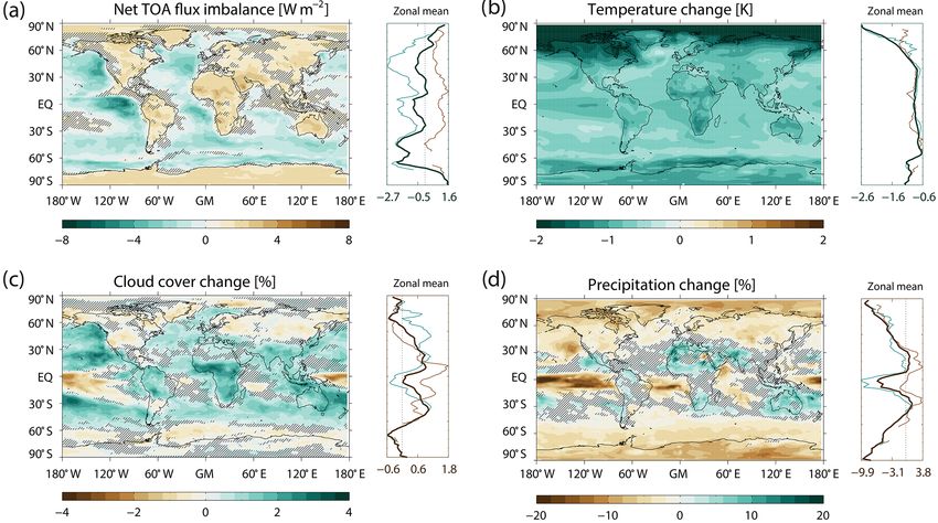
622                                   C. W. Stjern et al.: Response to marine cloud brightening in a multi-model ensemble

as geoengineering, could be considered as part of a response        ing that MCB might help stabilize the West Antarctic Ice
portfolio to contribute to reach such targets. Climate engi-        Sheet. However, comparison between studies has been dif-
neering can be defined as the deliberate modification of the        ficult partly due to different experimental design. Also, in
climate in order to alleviate negative effects of anthropogenic     studies based on one or only a few models, results will be
climate change (Sheperd, 2009). Marine cloud brightening            very dependent on the particular models’ parametrizations.
(MCB) is one such technique (Latham, 1990), which falls             For instance, Connolly et al. (2014) suggested that the unin-
into the category of solar radiation management or albedo           tended warming found in Alterskjær and Kristjánsson (2013)
modification, and aims to cool the climate by increasing the        for seeding of some particle sizes (as mentioned above) was
amount of solar radiation reflected by the Earth.                   likely to be an artifact of the cloud parametrization scheme in
   The MCB method involves adding suitable cloud conden-            the model used. To alleviate some of these issues, the Geo-
sation nuclei (CCN), for instance sea salt, into the marine         engineering Model Intercomparison Project (GeoMIP) ini-
boundary layer. As existing cloud droplets tend to distribute       tiated a series of experiments where a number of models
themselves on the available nuclei, a larger number of CCN          were to simulate MCB in a particular manner, with differ-
has the potential to enhance the cloud droplet number con-          ent degrees of complexity in the simulation design (Kravitz
centration (CDNC) in a cloud, which (given constant liquid          et al., 2013). The G1ocean-albedo experiment prescribes an
water paths) can reduce the droplet sizes and therefore in-         increase in ocean albedo in the models at a rate intended to
crease the cloud albedo (Twomey, 1974). In reality, however,        offset increasing global temperatures in response to a quadru-
the end result of adding CCN to the marine boundary layer           pling of atmospheric CO2 concentrations. The G4cdnc ex-
is highly uncertain, as there are many processes involved –         periment investigated in this work simulates a 50 % increase
each of which has a number of dependencies and uncertain-           in the CDNC of low marine clouds as described in more de-
ties. For instance, Alterskjær and Kristjánsson (2013) simu-        tail in Sect. 2. Finally, the G4sea-salt experiment involves an
lated sea-salt seeding of marine clouds using the Norwegian         increase in sea-salt emissions over tropical oceans at a rate
Earth System Model (NorESM) and found that for seeding              intended to produce a radiative forcing of −2.0 W m−2 under
particles above or below given size thresholds, a strong com-       the RCP4.5 scenario. The three experiments have an increas-
petition effect ultimately led to a warming of the climate,         ing degree of complexity or realistic representation.
contrary to the intention. Chen et al. (2012) studied obser-           Less idealized experiments, such as sea-salt injection sim-
vations of ship tracks and found that the magnitude and even        ulations, will include more of the processes in play between
the sign of the albedo response is dependent on the mesoscale       geoengineering and climate impacts. Such experiments have
cloud structure, the free tropospheric humidity, and cloud          taught us, for instance, that a substantial part of the cooling
top height. Similarly, Wang et al. (2011), using the WRF            will originate from direct aerosol effects, and that the indirect
model, found that the effectiveness of cloud albedo enhance-        cloud effects are just part of a number of responses of the
ment is strongly dependent on meteorological conditions and         climate system (Ahlm et al., 2017; Alterskjær et al., 2012;
background aerosol concentrations. There is therefore a great       Partanen et al., 2012). In order to get a clearer understanding
need for more studies of the processes behind and possible          of the causes of the inter-model spread in cloud response,
effects of MCB.                                                     we therefore look more closely into the simpler experiment
   Existing model studies of MCB (e.g., Alterskjær et al.,          G4cdnc, where only perturbations to cloud simulations are
2013; Bala et al., 2011; Bower et al., 2006; Jones et al., 2009;    made. The justification for performing more simplified sim-
Latham et al., 2014; Philip et al., 2009; Stuart et al., 2013;      ulations such as G4cdnc is that many models may partici-
Wang et al., 2011) have shed some light on potential benefits       pate, giving a more complete multi-model ensemble, but also
(e.g., in terms of climate cooling) as well as drawbacks (e.g.,     that the spatial climate response in near-surface air temper-
hydrological cycle changes). For instance, while all of the         ature and precipitation where CDNC are perturbed directly
above studies show that MCB “works” in terms of cooling             in a single fully coupled GCM is similar to that when sea-
climate, a spin-down of the hydrological cycle in the cooler        salt aerosol microphysics are included explicitly (Jones et al.,
climate leads to reduced precipitation in the global average,       2009; Jones and Haywood, 2012). In this paper we provide
with potential detrimental effects to humans and vegetation         an initial overview of the climate response in the G4cdnc ex-
(Muri et al., 2015). Jones et al. (2009) found a significant dry-   periment with a particular focus on the atmosphere. Our main
ing for the Amazon basin from increasing CDNC in marine             goal is to determine the range of responses associated with
stratocumulus decks. Bala et al. (2011) noted that differential     such a forcing and furthermore to assess the extent to which
cooling of oceans (where clouds were modified) versus land          the climate effects are dependent on the quantity, type, and
might result in circulation changes (seen also in Alterskjær        location of clouds.
et al., 2013) involving sinking motion over oceans and ris-            In the next section, we describe the G4cdnc experimental
ing motion over land, which therefore might experience an           design, and the data analysis approach. Section 3 reviews the
increase in precipitation. Thus, MCB may have very differ-          model climatologies, with a particular focus on differences in
ent regional effects. For instance, Latham et al. (2014) in-        clouds. Results from the climate engineering experiment are
vestigated possible beneficial regional effects of MCB, find-

Atmos. Chem. Phys., 18, 621–634, 2018                                                  www.atmos-chem-phys.net/18/621/2018/
C. W. Stjern et al.: Response to marine cloud brightening in a multi-model ensemble                                                           623

Table 1. Information on the contributing models, including resolution, number of realizations and their representation of the aerosol indirect
effect.

       Model                No. of         No. of vert.         RCP4.5/        Representation of aerosol indirect effect
                            grid cells     layers               G4cdnc
                            (lat × long)   (type)               realizations
       BNU-ESM              64 × 128       26 (hybrid sigma)    1/1            Single-moment microphysics scheme; Rasch and
                                                                               Kristjánsson (1998) with modification by Zhang et
                                                                               al. (2003). NOTE: to achieve effects of 50 % increase
                                                                               of CDNC over ocean regions below 680 hPa, a direct
                                                                               alteration of liquid droplet size by dividing (1.5(1/3) ) is
                                                                               done.
       CanESM2              64 × 128       35 (hybrid sigma)    5/3            Prognostic microphysics scheme accounting for the first
                                                                               indirect effect but not the second indirect effect (von
                                                                               Salzen et al., 2013)
       CSIRO-Mk3L-1-2       56 × 64        18 (hybrid sigma)    3/3            Prescribed CDNC
       GISS-E2-R            90 × 144       21 (hybrid sigma)    3/3            Prognostic calculations of CDNC (Menon et al., 2010),
                                                                               based on Morrison and Gettelman (2008)
       HadGEM2-ES           145 × 192      38 (hybrid height)   4/1            Diagnostic CDNC scheme based on Jones et al. (2001)
       IPSL-CM5A-LR         96 × 96        39 (hybrid sigma)    4/1            CDNC is computed from the total mass of soluble
                                                                               aerosol through the prognostic equation from Boucher
                                                                               and Lohmann (1995).
       MIROC-ESM            64 × 128       80 (hybrid sigma)    1/1            Prognostic calculation of CDNC (Abdul-Razzak and
                                                                               Ghan, 2000)
       MPI-ESM1-LR          96 × 192       47 (hybrid sigma)    1/1            Prescribed CDNC
       NorESM1-M            96 × 144       26 (hybrid sigma)    1/1            Double-moment microphysics scheme with prognostic
                                                                               calculation of CDNC (Abdul-Razzak and Ghan, 2000;
                                                                               Hoose et al., 2009; Morrison and Gettelman, 2008)

presented in Sect. 4, Sect. 5 provides the discussion, whilst            terminated, and the simulations are continued for a further
conclusions are drawn in Sect. 6.                                        20 years (until 2089) to assess the termination effect. Nine
                                                                         CMIP5 models participated in the experiment. However, the
                                                                         termination period was only investigated in six of the models.
2     Data and methods                                                   See Table 1 for a list of participating models.
                                                                            In the aforementioned G4sea-salt experiment, sea-salt par-
2.1    The G4cdnc experiment design                                      ticles are injected close to the ocean surface to simulate the
                                                                         entire life-cycle from aerosol injections to climate effects
The G4cdnc experiment uses the CMIP5 (Coupled Model In-
                                                                         (Ahlm et al., 2017). The G4cdnc experiment, however, sim-
tercomparison Project 5) RCP4.5 (Taylor et al., 2012) sce-
                                                                         plifies the process and addresses the adjustment of CDNC
nario as its baseline. RCP4.5 is the middle-of-the-road sce-
                                                                         without an actual increase in any cloud condensation nuclei
nario and assumes continued greenhouse gas emission in-
                                                                         (CCN) from sea spraying. Consequently, the resulting cli-
creases from today’s levels (albeit at reduced rate from a no-
                                                                         mate effects will only include aerosol–cloud interactions and
policy scenario like RCP8.5), followed by a decrease from
                                                                         will not include aerosol–radiation interactions (Boucher et
year 2040 and stabilization by year 2100, at which time
                                                                         al., 2013) or the climate system’s adjustments to them. Note
the anthropogenic radiative forcing amounts to 4.5 W m−2
                                                                         also that for BNU-ESM, the model design precluded a di-
above preindustrial levels (Meinshausen et al., 2011). The
                                                                         rect change in the CDNC. Therefore, instead of multiplying
G4cdnc experiment starts the climate engineering in year
                                                                         CDNC by 1.5 to obtain the 50 % increase, they had to ap-
2020, and prescribes a 50 % increase in the CDNC of ma-
                                                                         proximate the cloud seeding through a direct alteration of
rine low clouds. Marine low clouds are defined as clouds be-
                                                                         liquid droplet sizes (droplet radii are multiplied by the fac-
low 680 hPa over ocean grid boxes at all latitudes, except
                                                                         tor 1.51/3 ), which means that its experiment setup is slightly
where sea ice is present. The experiment is run for 50 years,
                                                                         different from the other models.
from 2020 to 2069, after which the cloud brightening is

www.atmos-chem-phys.net/18/621/2018/                                                           Atmos. Chem. Phys., 18, 621–634, 2018
624 C. W. Stjern et al.: Response to marine cloud brightening in a multi-model ensemble
Table 2. Global averages for the 20 first years (2006–2025) of the RCP4.5 experiment. Model spread is given as one standard deviation.
“Low cloud cover” is calculated using a random overlap assumption for all vertical levels below 680 hPa.
Total cloud cover Precipitation Liquid water path Low cloud cover
(%) (mm day−1 ) (g m−2 ) (%)
BNU-ESM 52.74 2.89 151.15 77.54
CanESM2 60.80 2.78 119.07 57.69
CSIRO-Mk3L-1-2 66.98 2.76 118.38 59.97
GISS-E2-R 61.01 3.22 192.71 31.19
HadGEM2-ES 53.32 3.09 92.14 –
IPSL-CM5A-LR 56.67 2.76 68.11 46.06
MIROC-ESM 50.37 2.82 139.28 55.88
MPI-ESM-LR 61.93 2.88 62.85 49.59
NorESM1-M 53.94 2.83 142.47 73.29
Model average and spread 57.5 (±5.4) 2.9 (±0.2) 120.7 (±41.6) 55.9 (±23.4)
Observations 68 (±3)a 2.68b 30–50 [10 to 100]c (not comparable to observations)
a As averaged from daytime measurements over several remote sensing datasets; see Stubenrauch et al. (2013). b Climatology for 1951–2000 from the Global
Precipitation Climatology Centre (Schneider et al., 2014). c Observations from NASA’s “A-Train” satellite observations (Jiang et al., 2012).
2.2 Postprocessing and analyses face air temperature change compared to the RCP4.5 sim-
ulations. Because of the timescales of the adjustments to the
applied forcing, we follow Williams et al. (2008) and Gre-
Some details of the nine contributing models can be seen
gory et al. (2004), using annual means for the first decade
in Table 1. For each model, annual averages are first cal-
and decadal means thereafter: the period of 2030–2069. This
culated from monthly mean model output and the ensem-
allows more weight to the years when the rapid adjustments
ble means over all available realizations are then calcu-
dominate, before the slow feedbacks have more impact in the
lated, before the data is regridded to a horizontal grid cor-
later part of the simulation.
responding to the average grid size of models: 2.1 × 2.7 lat-
itude × longitude. When calculating differences between the
G4cdnc experiment and the RCP4.5 scenario, we base our 3 Modeled cloud climatologies
analyses on years 2020–2069. To assess whether the differ-
ences between G4cdnc and RCP4.5 are statistically signif- Earth system models have large differences in their treat-
icant, a two-sample non-parametric Kolmogorov–Smirnov ment of clouds, as well as in their aerosol concentrations
(K-S) test (Conover, 1971) is used. and climatologies. The 5th assessment report of the Inter-
In our assessment, “low clouds” are quantified using a ran- governmental Panel on Climate Change (IPCC), similarly
dom overlap assumption, in which clouds in contiguous lay- to the previous ones, stressed the important role of clouds
ers overlap in a random way (Tian and Curry, 1989), based and their parameterizations in contributing towards the inter-
on the cloud cover for all grid cells from 1000 hPa and up to model spread in estimates of climate change (Stocker et al.,
680 hPa. Please note that this estimate is based on monthly 2013). As the G4cdnc experiment is designed so that changes
means, and these low cloud amounts will therefore not be are induced only to low clouds over ocean, we expect dif-
equal to the low cloud fractions calculating during model ferences in cloud fields to be a particularly large source of
runs (for models that does this); these numbers tend to be uncertainty in our results. This section therefore provides a
higher. However, they should give a fair representation of brief comparison of different climatological values between
geographical distribution, and numbers are comparable be- the models.
tween models. To estimate the effective radiative forcing In Table 2, a selection of cloud-related variables is given,
of increasing CDNC by 50 % in the different models, we based on global annual means from the first 20 years of
use the method of Gregory et al. (2004), whereby the top- the RCP4.5 simulation, to see how these values compare to
of-atmosphere (TOA) radiative flux imbalance is regressed present-day observations. Zonal mean cloud cover over the
against the globally averaged surface air temperature change same period is shown in Fig. 1. The lowermost row in Ta-
compared to the RCP4.5 simulations. To estimate the effec- ble 2 shows values from observations. Looking at the ob-
tive radiative forcing of increasing CDNC by 50 % in the dif- served cloud fraction of Fig. 1 (upper left panel), we see
ferent models, we use the method of Gregory et al. (2004), that low cloud amounts are particularly high near the poles,
whereby the global mean top of atmosphere radiative flux with also relatively high amounts extending towards the sub-
imbalance is regressed against the globally averaged sur- tropics and mid-latitudes, especially in the Southern Hemi-
Atmos. Chem. Phys., 18, 621–634, 2018 www.atmos-chem-phys.net/18/621/2018/C. W. Stjern et al.: Response to marine cloud brightening in a multi-model ensemble 625
CloudSat/CALIPSO Model median
(a) (b) 100
100
Cloud fraction [%]
15
75
Height (km)
Ice
9 50
25
3 Liquid
0 1000 0
60o S 30o S 0o N 30o N 60o N 60o S 30o S 0o N 30o N 60o N
(c)
NorESM1−M GISS−E2−R HadGEM2−ES
100 100 100
Pressure [hPa]
1000 1000 1000
60o S 30o S 0o N 30o N 60o N 60o S 30o S 0o N 30o N 60o N 60o S 30o S 0o N 30o N 60o N
BNU−ESM CanESM2 CSIRO−Mk3L−1−2
100 100 100
Pressure [hPa]
1000 1000 1000
60o S 30o S 0o N 30o N 60o N 60o S 30o S 0o N 30o N 60o N 60o S 30o S 0o N 30o N 60o N
IPSL−CM5A−LR MIROC−ESM MPI−ESM−LR
100 100 100
Pressure [hPa]
1000 1000 1000
60o S 30o S 0o N 30o N 60o N 60o S 30o S 0o N 30o N 60o N 60o S 30o S 0o N 30o N 60o N
Latitude Latitude Latitude
Figure 1. Panel (a) shows cloud fraction (%) from CloudSat/CALIPSO, adapted from Fig. 7.5c of Boucher et al. (2013) with permission.
Panel (b) shows the GeoMIP model median for the first 20 years of the RCP4.5 scenario, and panels in (c) show individual RCP4.5 GeoMIP
model results for the same years. Note different vertical axes for the AR5 and GeoMIP plots.
sphere. Observations show a high fraction of low stratocu- and a particular deficiency in subtropical low clouds. Like-
mulus clouds around 30◦ S (Wood, 2012), an area that, given wise, Konsta et al. (2016) compared tropical clouds in IPSL-
its distance from major pollution sources, might be partic- CM5A-LR to satellite observations and found an underesti-
ularly susceptible to cloud seeding (Alterskjær et al., 2013; mation of total cloud cover (underestimated low- and mid-
Jones et al., 2009; Partanen et al., 2012). It is therefore inter- level tropical clouds and overestimated high clouds) asso-
esting to note that several models are not able to realistically ciated with a high bias in cloud optical depth. Other mod-
reproduce these clouds. els have similar issues. For instance, Stevens et al. (2013)
Comparing individual model cloud fractions in Fig. 1 showed that MPI-ESM-LR has prominent negative biases in
(lower three rows) to the observed cloud fraction, we see that the major tropical stratocumulus regions. Although the low
few models compare well to the observed low-level cloud clouds in this study are an approximation as explained in
amounts. It is a well-known problem, commonly referred Sect. 2.2, a comparison between our Fig. 2 and the satellite-
to as the “too few, too bright” problem, that climate mod- based observations of low clouds in Fig. 1 of Cesana and
els tend to underestimate the amount of low clouds, while Waliser (2016) clearly demonstrates this. Although MPI-
concurrently overestimating their optical thickness, and Nam ESM-LR has a globally averaged cloud fraction close to the
et al. (2012) confirmed that this is true for most of the multi-model average (Table 2), there is a concentration of
CMIP5 models. Among the contributing G4cdnc models, clouds around the poles rather than at lower latitudes (see
GISS-E2-R and IPSL-CM5A-LR have particularly few low- Fig. 2). Brightening polar clouds may be less efficient than if
level clouds in the region around 30◦ S; see Fig. 1. This is the majority of clouds were located at lower latitudes, due to
stressed in Schmidt et al. (2014), who compared cloud data the low solar angle at high latitudes, although influences of
from GISS-E2-R to satellite measurements and found un- cloud changes on the long wave spectrum may still be large
derestimated cloud covers over mid-latitude ocean regions (Kravitz et al., 2014). Yet, as we will show in the next sec-
www.atmos-chem-phys.net/18/621/2018/ Atmos. Chem. Phys., 18, 621–634, 2018626 C. W. Stjern et al.: Response to marine cloud brightening in a multi-model ensemble
Figure 2. Low cloud fraction (%) for the first 20 years of the RCP4.5 scenario, for the model median as well as the individual models. Low
clouds are estimated using a random overlap assumption (Tian and Curry, 1989).
tion, the climate response of MPI-ESM-LR is still the highest in Sect. 2.2) of −1.91 [−0.58 to −2.48] W m−2 , where the
of all the models. numbers in brackets indicate model minimum and maxi-
In an evaluation of 19 CMIP5 models against NASA’s mum values; see Fig. 3a and Table 3. There is a factor of
“A-Train” satellites, Jiang et al. (2012) found a best esti- 4.3 difference between the highest and lowest model ERFs;
mate global mean observed liquid water path (LWP) of 30– while CSIRO-Mk3L-1-2 has the largest radiative forcing of
50 g m−2 , with an uncertainty range from 10 to 100 g m−2 . −2.48 W m−2 , GISS-E2-R has the weakest (−0.58 W m−2 ).
Table 2 shows a vast inter-model spread in annual aver- The models with a weak ERF typically also have a weak
age LWP. Values range from 61.7 g m−2 (MPI-ESM-R) to correlation between temperature change and change in TOA
194.7 g m−2 (GISS-E2-R). These variations in cloud thick- radiative flux imbalance (Table S1 in the Supplement). The
ness can be decisive to a model’s response to cloud seed- model median geographical pattern of this radiative pertur-
ing since (given similar levels of cloud condensation nuclei) bation is shown in Fig. 4a.
clouds with LWP above a certain level will be less suscepti- The negative forcing of increasing CDNC cools the near-
ble to changes in the number of cloud droplets (Sorooshian surface air temperatures with a model median of 0.96 [−0.17
et al., 2009). to −1.21] K, compared to the RCP4.5 scenario. Figure 3b
shows the time series from year 2020 to 2090 of the G4cdnc–
RCP4.5 difference in global mean near-surface air temper-
ature. The figure shows that NorESM1-M, GISS-E2-R and
4 Climate response to G4cdnc
IPSL-CM5A-LR are the models that yield the weakest tem-
The G4cdnc experiment results in a model median ERF (cal- perature response and these are the models with the weakest
culated using the Gregory regression method, as explained
Atmos. Chem. Phys., 18, 621–634, 2018 www.atmos-chem-phys.net/18/621/2018/C. W. Stjern et al.: Response to marine cloud brightening in a multi-model ensemble 627
Table 3. G4cdnc minus RCP4.5 difference (based on years 2020–2069) in the key variables, including the effective radiative forcing as
estimated in Fig. 3a). An asterisk denotes that the change is not significant at the 95 % level by the Kolmogorov-Smirnov test.
Gregory MCB Total cloud Temp. Precip. Liquid Low cloud
regression sensitivity cover change change water path cover
ERF change change change
Units W m−2 K W m−2 % K % g m−2 %
BNU-ESM −1.91 0.61 −0.46 −1.16 −2.72 +1.83 −0.01
CanESM2 −2.00 0.48 +0.29 −0.96 −2.28 −0.71 +1.82
CSIRO-Mk3L-1-2 −2.48 0.43 +1.17 −1.07 −2.93 +4.52 +2.00
GISS-E2-R −0.58 0.29 +0.05∗ −0.17 −0.61 −0.93 +0.16
HadGEM2-ES −1.93 0.49 +1.01 −0.96 −2.34 +0.01 –
IPSL-CM5A-LR −1.05 0.42 +1.03 −0.44 −1.70 −1.10 +1.28
MIROC-ESM −2.10 0.50 +0.36 −1.06 −2.51 −4.62 +1.55
MPI-ESM-LR −2.32 0.52 +0.78 −1.21 −2.96 +6.98 +5.95
NorESM1-M −0.89 0.35 +0.01 −0.31 −0.57 −0.61 +0.16
Ensemble median −1.91 (±0.63) 0.47 (±0.09) +0.18 (±0.42) −0.96 (±0.45) −2.35 (±0.92) −0.61 (±3.43) +1.55 (±1.93)
(a) Figure 4b shows the geographical pattern of the ensem-
0.5
Net TOA forcing change [W m -2 ]
0.0 NorESM1−M: −0.9 W m −2 ble median temperature difference between the G4cdnc and
GISS−E2−R: −0.6 W m −2
−0.5 HadGEM2−ES: −1.9 W m −2 RCP4.5 experiments, based on years 2020–2069 (for individ-
BNU−ESM: −1.9 W m −2
−1.0 CanESM2: −2.0 W m −2 ual models, see Fig. S1 in the Supplement). There is a strong
CSIRO−Mk3L−1−2: −2.5 W m −2
−1.5
IPSL−CM5A−LR: −1.1 W m −2 polar amplification of the cooling signal, with largest cooling
−2.0 MIROC−ESM: −2.1 W m −2
MPI−ESM−LR: −2.3 W m −2 over the Arctic from positive sea-ice feedback, and a some-
−2.5 Model median: −1.9 W m −2
−3.0 what weaker cooling around Antarctica. Individual model
0.0 −0.5 −1.0 −1.5 −2.0
Temperature change [K] numbers of the Arctic amplification is given in Table S2,
(b) but the median value is 1.9. Some of the models (NorESM1-
0.5
Temperature change [K]
0.0
M, BNU-ESM and MIROC-ESM) show a particularly large
spatial correlation (around −0.5 and significant at the 99 %
−0.5
level) between the magnitude of the cooling (averaged over
−1.0
2020–2069) and the baseline (averaged over the 20 first years
−1.5 of the RCP4.5 simulation) low cloud fractions; see Table S1.
−2.0 Such a tendency can also be seen in the ensemble median
2020 2030 2040 2050 2060 2070 2080 2090
Years temperature change of Fig. 4b; typical stratocumulus regions
such as parts of the tropical Atlantic Ocean and the Pacific
Figure 3. (a) Regression of global annual means of the net TOA Ocean off the coasts of Peru and the USA (Wood, 2012) show
radiative flux imbalance and near-surface temperatures for each
stronger cooling.
model (see Gregory et al., 2004). Each square represents global
Over oceans, the cooling also has a slight tendency to be
annual mean for each of the first 10 years and decadal means for
the remaining part of the simulations (i.e. last four decades, 2030– stronger in regions which have a low baseline LWP. Corre-
2069). Numbers to the right gives the intercept – i.e., the effective lations between the average change in temperature and the
radiative forcing. (b) Time series of the difference in global annual baseline LWP for each model gives the individual model cor-
mean near-surface temperature between G4cdnc and RCP4.5 for relation coefficients in Table S1, and correlations between
each model. Dotted vertical line indicates the onset of the termi- grid cell model medians of these quantities gives a spatial
nation period. correlation coefficient of 0.42 (significant at the 99 % level).
Such a tendency might indicate that cloud susceptibility, or
the potential of a cloud to produce cooling by increased
effective radiative forcing. Conversely, MPI-ESM-LR, with albedo in response to the increase in droplet numbers, is
the next largest forcing, shows the strongest cooling. larger in clouds that are not too dense to begin with. However,
Shown in Table 3 is also the “MCB sensitivity”, defined two of the models (NorESM1-M and BNU-ESM) have cor-
here as the global temperature change normalized by the relations of −0.30 and −0.47, respectively, indicating larger
ERF. We find a model median value of 0.47, with a much cooling in areas of larger water paths. Note also that changes
smaller inter-model spread (a factor of 1.8 difference be- in LWP are highly variable between models (Table 3 and
tween highest and lowest model value). MPI-ESM-LR and Fig. S2), with particularly strong positive changes for the two
BNU-ESM give the strongest cooling per degree forcing. models with prescribed CDNC (MPI-ESM-LR and CSIRO-
Mk3L-1-2). Although the CDNC is increased solely over the
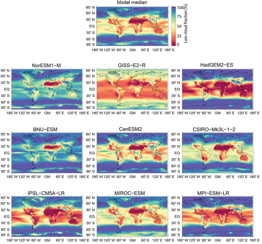
www.atmos-chem-phys.net/18/621/2018/ Atmos. Chem. Phys., 18, 621–634, 2018628 C. W. Stjern et al.: Response to marine cloud brightening in a multi-model ensemble Figure 4. Ensemble median (taken in each grid cell) G4cdnc-RCP4.5 difference based on years 2020–2069 of (a) TOA net radiative flux imbalance (W m−2 ), (b) near-surface air temperature change (K), (c) total cloud cover (%), and (d) precipitation (%). Hatched areas are grid cells where fewer than 75 % of the models agreed on the sign of the change. Zonal averages are given to the right of each panel, where brown and blue lines indicate land-only and ocean-only averages. See Figs. S2 and S3 in the Supplement for individual model changes in cloud cover and precipitation, respectively. oceans, the land masses, particularly at low latitudes, cool Fig. S4). Both total cloud cover and precipitation show dis- more than the ocean regions. We find that land areas between tinct differences in land/sea responses. Specifically, the cloud 35◦ S and 35◦ N cool by 1.08 K, while low-latitude ocean ar- cover between 35◦ S and 35◦ N tends to increase more over eas cool by 0.83 K. land (2.15 %) than over the ocean (0.32 %). While precip- As a consequence of the cooling climate, there is a weak- itation increases by 1.2 % over land, there is for the same ening of the hydrological cycle resulting in a decreasing latitudes a drying of 3.8 % for the oceans, over which the ap- global mean precipitation of −2.35 [−0.57 to −2.96] %. As plied geoengineering causes suppression of evaporation (not expected, the model with the strongest cooling has the largest shown). reduction in global precipitation. The total cloud cover in- Figure 5a shows changes in outgoing shortwave radia- creases in all models but BNU-ESM, and there is a strong tion at TOA, while Fig. 5b shows outgoing longwave radi- and statistically significant correlation (coefficient of −0.71) ation (OLR). The increase in outgoing shortwave radiation between how much the global mean cloud cover changes for is strongest in ocean regions typically associated with low a model and its baseline fraction of low clouds. The model clouds, and it changes little over land. In contrast, the OLR median cloud covers (Fig. 4c) are reduced in high northern has a band of increases around the ITCZ, but otherwise de- and southern latitudes due to the particularly strong cooling creases. The decrease is most pronounced near the poles, but and increase in sea ice in these regions (see Fig. S3 for indi- also over tropical land masses. Figure 5c shows that the low vidual total cloud change patterns). Clouds are also reduced cloud cover (see Fig. S5 for individual model changes) gener- over large regions of mid-latitude land masses, such as over ally has a pattern similar to the total cloud cover change, and Russia, northern Europe and North America, and in the In- seems to be a dominant cause of the changes we see in out- tertropical Convergence Zone (ITCZ). Changes in precipi- going shortwave radiation (a significant spatial correlation of tation (Fig. 4d) is mostly correlated to the cloud changes, 0.35 is found between Fig. 5a and c). Figure 5d, on the other with notable exceptions being the northern Pacific and At- hand, shows that high clouds increase primarily over tropi- lantic, where precipitation is reduced in spite of an increase cal and subtropical land masses, producing the reduction in in clouds. In contrast to the marine stratocumulus geoengi- OLR. This is from increasing convection over land, produc- neering experiment in Jones et al. (2009) only two mod- ing more anvils and ice clouds, as also reflected in the en- els (MPI-ESM-LR and IPSL-CM5A-LR) show drying over hancement of precipitation in these areas. The model-median the Amazon (see individual precipitation change patterns in Atmos. Chem. Phys., 18, 621–634, 2018 www.atmos-chem-phys.net/18/621/2018/
C. W. Stjern et al.: Response to marine cloud brightening in a multi-model ensemble                                                    629

Figure 5. Ensemble median (taken in each grid cell) G4cdnc–RCP4.5 difference of years 2020–2069 of (a) outgoing shortwave radiation
at TOA (W m−2 ), (b) outgoing longwave radiation at TOA (W m−2 ), (c) change in low cloud fraction (%), and (d) change in high cloud
fraction (%). Hatched areas are grid cells where fewer than 75 % of the models agreed on the sign of the change. Zonal averages are given to
the right of each panel, where brown and blue lines indicate land-only and ocean-only averages, respectively.

spatial correlation between OLR and change in high clouds               (where the latter is the termination period), there was a strong
is −0.55 and highly significant.                                        Arctic amplification when looking at the RCP4.5 scenario,
   The ability of ecosystems to adapt, and the risk for extinc-         but a weaker amplification in the climate engineering sce-
tion, dramatically increases under rapid climate change (e.g.,          nario. Consistently with this, we find that the model median
Jump and Peñuelas, 2005; Menéndez et al., 2006). One of the             Arctic amplification is 3.6 for the RCP4.5 scenario and 1.7
concerns regarding climate engineering is the possibility that,         for G4cdnc, for the same years (see Table S2). The pattern
due to unforeseen events or government issues, there may                of change in the termination period (Fig. S5) is broadly just a
be a sudden suspension of the climate engineering efforts,              reversal of the geographical patterns seen in Fig. 4. However,
casting Earth’s climate into a phase of rapid re-warming.               the spread between the models, as indicated by the hatching
This termination effect has been investigated in several stud-          in the maps, is much larger for the termination effect precip-
ies (Aswathy et al., 2015; Jones et al., 2013; Matthews and             itation response than for the temperature response, as found
Caldeira, 2007). As mentioned in Sect. 2.1, six models in the           also in Jones et al. (2013).
present study simulated the termination effect by turning off
the CDNC perturbation and continuing the simulations for
20 years. The effect on global temperatures (relative to the            5   Discussion
RCP4.5 scenario) in this termination period can be seen in
the last 20 years in Fig. 3b. At the end of these 20 years,             Increasing CDNC in low marine clouds results in global
temperatures are almost back at the RCP4.5 levels. Previous             cooling. This is accompanied by a global mean reduction in
GeoMIP publications investigating stratospheric aerosol in-             precipitation. These signals are robust across all nine mod-
jections (see, e.g., Berdahl et al., 2014) have noted a much            els, but the magnitude of the change varies by 50 % between
faster warming in the rebound or termination period than in             models for the temperature change, and by 40 % for the pre-
the RCP4.5 scenario, and this we find also here: for years              cipitation change.
2070 to 2090 there is a warming of 0.007 K yr−1 for RCP4.5                 Although the CDNC is only increased over oceans, we find
and a warming of 0.040 K yr−1 for G4cdnc. In a GeoMIP                   stronger cooling over land masses, particularly in the lower
study of stratospheric aerosol injections using three global            latitudes. High clouds increase the most over low-latitude
climate models, Aswathy et al. (2015) find that comparing               land, and the OLR is reduced over low-latitude land and in-
the mean temperatures of the years 2050–2069 to 2020–2079               creases over oceans. This is consistent with a shift in con-
                                                                        vection from ocean to land, which also explains the increase

www.atmos-chem-phys.net/18/621/2018/                                                         Atmos. Chem. Phys., 18, 621–634, 2018
630 C. W. Stjern et al.: Response to marine cloud brightening in a multi-model ensemble in precipitation of +1.2 % over low-latitude land as opposed with respect to further changes in droplet numbers, in line to a drying of −3.8 % over oceans. This kind of pattern with the findings of Painemal and Minnis (2012) mentioned has been seen in previous modeling studies of marine cloud above. brightening. For instance, Bala et al. (2011) used an Earth Geoffroy et al. (2017) investigated the role of different system model to perform simulations where the effective stratiform cloud schemes to the inter-model spread of cloud droplet size in liquid clouds was reduced over oceans glob- feedbacks, looking at 14 models – four of which were used in ally. They found that the differential enhancement of albedo the present study. They found that NorESM1-M, which diag- over oceans and land triggered a monsoonal circulation with noses stratiform clouds based on relative humidity and atmo- rising motion over land and sinking motion over oceans. This spheric stability, had an opposite cloud feedback from mod- happened as the vertically integrated air mass cooled more els (including HadGEM2-ES, CSIRO-Mk3L-1-2 and IPSL- over the oceans where the cloud albedo was increased than CM5A-LR) that diagnoses such clouds based solely on rel- over land. The resulting density change caused an increase ative humidity. BNU-ESM, whose change in TOA radiative in net land to ocean transport above 400 hPa and an increase flux imbalance is that of the model median, uses the same in the net ocean to land transport below 400 hPa. Alterskjær stratiform cloud scheme as NorESM1-M (Ji et al., 2014), and et al. (2013) analyzed an ensemble of three Earth system like NorESM1-M the change in low cloud cover is near zero. models that are all included in the present study and noted It does not, however, have the negative change in LWP seen the same land–sea difference in warming and associated hy- in NorESM1-M. This may be due to the specific setup of the drological cycle changes. Similarly, Niemeier et al. (2013) simulations in BNU-ESM, where to obtain the 50 % decrease compared three types of solar radiation management (strato- in CDNC a direct alteration of liquid droplet size was done. spheric sulfur injections, mirrors in space and MCB) and In terms of TOA radiative flux imbalance, CSIRO-Mk3L-1-2 found that only the MCB experiment induced changes to the has the strongest response of all models. LWP, amount of low Walker circulation. clouds, and the geographical distribution of low clouds, how- Marine cloud brightening through emissions of some ever, are all similar to the model average. The model has the agent, for instance sea salt, into the marine boundary layer strongest cooling per forcing (ERF) and shows the strongest influences the low-lying clouds. But we find that the amount increase in low cloud cover. and location of clouds vary greatly between the models, As seen in Table 1, there are large differences be- which will cause variation in their response to MCB (see, tween models as to how the aerosol–cloud processes are e.g., Chen and Penner, 2005, who found cloud fraction to be parametrized, and this presumably has an impact on the MCB one of the most important sources of uncertainty in model- climate response. For instance, Morrison et al. (2009) found differences in estimates of the first indirect effect). We also that the complexity of the cloud schemes had large impacts find a substantial inter-model spread in the LWP, which is on stratiform precipitation; Penner et al. (2006) compared one of the factors determining how susceptible a cloud is to several models and concluded that the method of parameter- albedo changes through the Twomey effect (Twomey, 1974). ization of CDNC can have a large impact on the calculation For instance, MPI-ESM-LR has a fraction of low clouds that of the first indirect effect. CSIRO-Mk3L-1-2 and MPI-ESM- is close to the model average, but a geographical distribution LR are the only models that have prescribed CDNC levels in of those low clouds that could imply a reduced efficiency of their simulations, and these models stand out as having ERFs the CDNC enhancement. Low clouds at higher latitudes are well above any of the other models. While an evaluation of less effective at cooling, as the solar angle, and hence the which liquid cloud parametrizations are more appropriate is climate effect, is lower. MPI-ESM-LR also has the lowest beyond the scope of this paper, this might be an indication globally averaged LWP of all models. The potential that an that prescribing CDNC levels may lead to exaggerated re- increase in CDNC has to enhance the cloud albedo (the cloud sponses to marine cloud brightening. albedo susceptibility) has been shown to be smaller in clouds A caveat of the present study is that the spatial resolu- with low LWP. For instance, Painemal and Minnis (2012) in- tion of global climate models is too coarse to resolve im- vestigated satellite data for typical stratocumulus regions and portant processes such as convection or precipitation forma- found an increase in cloud albedo susceptibility with LWP up tion. These processes are instead parametrized, which may to about 60 g m−2 , after which the susceptibility leveled off lead to unknown artifacts in the responses, dependent on or even decreased slightly. Even so, this model has the sec- the specific formulations used (see, e.g., Clark et al., 2009, ond strongest ERF of all the models, possibly due to a very who compared precipitation forecast skills for convection- strong increase in cloud amounts between around 40◦ S to allowing and convective-parametrized ensembles). It is also 40◦ N. GISS-E2-R, on the other hand, is the model with the important to point out that the G4cdnc experiment was not weakest ERF. We find that this model has the smallest low designed to give a realistic representation of the magnitude cloud fractions among all the models, and there is also a ten- of cooling and other climate responses to MCB, but rather dency for these clouds to be concentrated at higher latitudes. to test the robustness of models in simulating geographically In addition, the LWP is extremely high, which could con- heterogeneous radiative flux changes and to see their effects ceivably mean that the clouds are already relatively saturated on climate. Increasing CDNC by 50 % over all oceans is Atmos. Chem. Phys., 18, 621–634, 2018 www.atmos-chem-phys.net/18/621/2018/
C. W. Stjern et al.: Response to marine cloud brightening in a multi-model ensemble                                             631

clearly an exaggeration of what could credibly be done. A         found for G4sea-salt that the direct effect (aerosol–radiation
more realistic GeoMIP marine cloud brightening experiment,        effect) of the sea-salt aerosols themselves contributes signif-
G4sea-salt, is analyzed by Ahlm et al. (2017). Their results      icantly to the total radiative effect of sea-salt climate engi-
show what areas in the participating models where the sea-        neering. It should be noted that even experiments that cap-
salt seeding is the most effective at brightening the clouds.     ture this direct effect may be subject to biases caused by pro-
This includes the decks of persistent low-level clouds off the    cesses not included in the experiments. For instance, Stuart
west coasts of the major continents in the subtropics. Alter-     et al. (2013) noted that sea-spray climate engineering studies
skjær et al. (2012) investigated the susceptibility of marine     assume a uniform distribution of the emitted sea salt in ocean
clouds to MCB based on satellite as well as model data and        grid boxes, which does not account for sub-grid aerosol co-
reached a similar conclusion; large regions between 30◦ S         agulation within sea-spray plumes. They find that accounting
and 30◦ N, and especially clean regions in the Pacific and In-    for this effect reduces the CDNC (and the resulting radiative
dian oceans, along with regions in the western Atlantic, were     effect) by about 50 % over emission regions, with variations
susceptible.                                                      from 10 to 90 % depending on meteorological conditions.
                                                                     Cloud feedbacks remain the largest source of inter-model
                                                                  spread in predictions of future climate change (Vial et al.,
6   Summary and conclusion                                        2013). While detailed, high-resolution simulations of marine
                                                                  sky brightening give crucial insights into processes that con-
Nine models have conducted a coordinated idealized ma-            tribute to the total climate response, multi-model idealized
rine cloud brightening experiment G4cdnc of the GeoMIP            experiments such as the G4cdnc are still important to un-
project, producing a median ERF of −1.91 [−0.58 to                tangle the cloud responses. We hypothesize that liquid cloud
−2.48] W m−2 . While climate in general cools as intended,        parameterizations ought to be of appropriate complexity in
there are large geographical variations in the climate re-        order to attempt to model marine cloud brightening and the
sponse. For instance, although the global cooling leads to a      climate response.
general drying, robust model responses also include a slight
precipitation increase over low-latitude land regions, such as
subtropical Africa, Australia and large parts of South Amer-      Data availability. All model data are available through the Earth
ica. This is a result of the land–sea contrast in tempera-        System Grid or upon request to the contact author.
ture initiated by brightening clouds only over ocean regions,
which results in a circulation pattern with rising motion over
land and sinking air over ocean, particularly over lower lati-    The Supplement related to this article is available online
tudes.                                                            at https://doi.org/10.5194/acp-18-621-2018-supplement.
   Responses in precipitation and clouds show particularly
large inter-model spreads. For some models we find a strong
dependency of the climate response on the location of low
clouds in the baseline simulation, RCP4.5, and also on the        Competing interests. The authors declare that they have no conflict
thickness in terms of LWP of the clouds. For other models no      of interest.
such clear dependency is found. Variations in the complex-
ity of microphysical schemes contribute to the large model
spread in responses, with an apparent tendency for stronger       Special issue statement. This article is part of the special issue
responses for the more simple representations. Conceivably,       “The Geoengineering Model Intercomparison Project (GeoMIP):
the more realistically the processes between CDNC pertur-         Simulations of solar radiation reduction methods (ACP/GMD inter-
bation and cloud albedo change are simulated, the more            journal SI)”. It is not associated with a conference.
buffering processes are included, dampening the total cli-
mate response (Stevens and Feingold, 2009). Indeed, climate
changes from G4cdnc do not include all processes in play          Acknowledgements. The work of Jón Egill Kristjánsson,
between seeding of the clouds and the actual climate re-          Camilla W. Stjern, Helene Muri and Lars Ahlm was sup-
sponse even in the models with the most advanced micro-           ported by the EXPECT project, funded by the Norwegian Research
physics schemes. While the increase in CDNC is assumed to         Council, grant no. 229760/E10. Camilla W. Stjern wishes to
                                                                  thank CICERO for letting her continue and complete the present
originate from an increase in for instance sea-salt particles
                                                                  project. Helene Muri was also funded by RCN grant 261862/E10.
in the marine boundary layer, one caveat with the G4cdnc
                                                                  Lars Ahlm was also supported by the Swedish Research Council
experiment is that it does not simulate these particles specif-   FORMAS (grant 2015-748). The Pacific Northwest National
ically. This is, however, done in the follow-up experiment        Laboratory is operated for the US Department of Energy by
G4sea-salt, which was performed by three of the models in-        Battelle Memorial Institute under contract DE-AC05-76RL01830.
vestigated here. Consistent with previous findings (Jones and     Steven J. Phipps was supported by the Australian Research
Haywood, 2012; Partanen et al., 2012), Ahlm et al. (2017)         Council’s Special Research Initiative for the Antarctic Gateway

www.atmos-chem-phys.net/18/621/2018/                                                  Atmos. Chem. Phys., 18, 621–634, 2018
632 C. W. Stjern et al.: Response to marine cloud brightening in a multi-model ensemble
Partnership (project ID SR140300001). The work of Duoying Ji Bower, K., Choularton, T., Latham, J., Sahraei, J., and Salter,
and John C. Moore was supported by the National Basic Research S.: Computational assessment of a proposed technique
Program of China (grant number 2015CB953600). for global warming mitigation via albedo-enhancement of
marine stratocumulus clouds, Atmos. Res., 82, 328–336,
Edited by: Lynn M. Russell https://doi.org/10.1016/j.atmosres.2005.11.013, 2006.
Reviewed by: two anonymous referees Cesana, G. and Waliser, D. E.: Characterizing and understand-
ing systematic biases in the vertical structure of clouds in
CMIP5/CFMIP2 models, Geophys. Res. Lett., 43, 10538–10546,
https://doi.org/10.1002/2016GL070515, 2016.
References Chen, Y. and Penner, J. E.: Uncertainty analysis for estimates of the
first indirect aerosol effect, Atmos. Chem. Phys., 5, 2935–2948,
Abdul-Razzak, H. and Ghan, S. J.: A parameterization of aerosol https://doi.org/10.5194/acp-5-2935-2005, 2005.
activation: 2. Multiple aerosol types, J. Geophys. Res.-Atmos., Chen, Y.-C., Christensen, M. W., Xue, L., Sorooshian, A., Stephens,
105, 6837–6844, https://doi.org/10.1029/1999JD901161, 2000. G. L., Rasmussen, R. M., and Seinfeld, J. H.: Occurrence of
Ahlm, L., Jones, A., Stjern, C. W., Muri, H., Kravitz, B., and lower cloud albedo in ship tracks, Atmos. Chem. Phys., 12,
Kristjánsson, J. E.: Marine cloud brightening – as effec- 8223–8235, https://doi.org/10.5194/acp-12-8223-2012, 2012.
tive without clouds, Atmos. Chem. Phys., 17, 13071–13087, Clark, A. J., Gallus Jr., A., Xue, M., and Kong, F.: A
https://doi.org/10.5194/acp-17-13071-2017, 2017. Comparison of Precipitation Forecast Skill between
Alterskjær, K. and Kristjánsson, J. E.: The sign of the radiative Small Convection-Allowing and Large Convection-
forcing from marine cloud brightening depends on both parti- Parameterizing Ensembles, Weather Forecast., 24, 1121–1140,
cle size and injection amount, Geophys. Res. Lett., 40, 210–215, https://doi.org/10.1175/2009WAF2222222.1, 2009.
https://doi.org/10.1029/2012GL054286, 2013. Connolly, P. J., McFiggans, G. B., Wood, R., and Tsiamis, A.: Fac-
Alterskjær, K., Kristjánsson, J. E., and Seland, Ø.: Sensitivity tors determining the most efficient spray distribution for ma-
to deliberate sea salt seeding of marine clouds – observations rine cloud brightening, Philos. T. R. Soc. A, 372, 20140056,
and model simulations, Atmos. Chem. Phys., 12, 2795–2807, https://doi.org/10.1098/rsta.2014.0056, 2014.
https://doi.org/10.5194/acp-12-2795-2012, 2012. Conover, W. J.: Practical Nonparametric Statistics, John Wiley &
Alterskjær, K., Kristjánsson, J. E., Boucher, O., Muri, H., Sons, New York, 309–314, 1971.
Niemeier, U., Schmidt, H., Schulz, M., and Timmreck, Geoffroy, O., Sherwood, S. C., and Fuchs, D.: On the role
C.: Sea-salt injections into the low-latitude marine bound- of the stratiform cloud scheme in the inter-model spread
ary layer: The transient response in three Earth sys- of cloud feedback, J. Adv. Model. Earth Sy., 9, 423–437,
tem models, J. Geophys. Res.-Atmos., 118, 12195–12206, https://doi.org/10.1002/2016MS000846, 2017.
https://doi.org/10.1002/2013JD020432, 2013. Gregory, J. M., Ingram, W. J., Palmer, M. A., Jones, G. S.,
Aswathy, V. N., Boucher, O., Quaas, M., Niemeier, U., Muri, H., Stott, P. A., Thorpe, R. B., Lowe, J. A., Johns, T. C., and
Mülmenstädt, J., and Quaas, J.: Climate extremes in multi-model Williams, K. D.: A new method for diagnosing radiative forc-
simulations of stratospheric aerosol and marine cloud brighten- ing and climate sensitivity, Geophys. Res. Lett., 31, L03205,
ing climate engineering, Atmos. Chem. Phys., 15, 9593–9610, https://doi.org/10.1029/2003GL018747, 2004.
https://doi.org/10.5194/acp-15-9593-2015, 2015. Hoose, C., Kristjánsson, J. E., Iversen, T., Kirkevåg, A., Seland, Ø.,
Bala, G., Caldeira, K., Nemani, R., Cao, L., Ban-Weiss, G., and and Gettelman, A.: Constraining cloud droplet number concen-
Shin, H.-J.: Albedo enhancement of marine clouds to counteract tration in GCMs suppresses the aerosol indirect effect, Geophys.
global warming: impacts on the hydrological cycle, Clim. Dy- Res. Lett., 36, L12807, https://doi.org/10.1029/2009GL038568,
nam., 37, 915–931, https://doi.org/10.1007/s00382-010-0868-1, 2009.
2011. Ji, D., Wang, L., Feng, J., Wu, Q., Cheng, H., Zhang, Q., Yang,
Berdahl, M., Robock, A., Ji, D., Moore, J. C., Jones, A., J., Dong, W., Dai, Y., Gong, D., Zhang, R.-H., Wang, X., Liu,
Kravitz, B., and Watanabe, S.: Arctic cryosphere response J., Moore, J. C., Chen, D., and Zhou, M.: Description and ba-
in the Geoengineering Model Intercomparison Project G3 sic evaluation of Beijing Normal University Earth System Model
and G4 scenarios, J. Geophys. Res.-Atmos., 119, 1308–1321, (BNU-ESM) version 1, Geosci. Model Dev., 7, 2039–2064,
https://doi.org/10.1002/2013JD020627, 2014. https://doi.org/10.5194/gmd-7-2039-2014, 2014.
Boucher, O. and Lohmann, U.: The sulface-CCN-cloud albedo Jiang, J. H., Su, H., Zhai, C., Perun, V. S., Del Genio, A.,
project. A sensitivity study with two general circulation models, Nazarenko, L. S., Donner, L. J., Horowitz, L., Seman, C., Cole,
Tellus, 478, 281–300, 1995. J., Gettelman, A., Ringer, M. A., Rotstayn, L., Jeffrey, S., Wu,
Boucher, O., Randall, D., Artaxo, P., Bretherton, C., Feingold, G., T., Brient, F., Dufresne, J.-L., Kawai, H., Koshiro, T., Watan-
Forster, P., Kerminen, V.-M., Kondo, Y., Liao, H., Lohmann, U., abe, M., LÉcuyer, T. S., Volodin, E. M., Iversen, T., Drange, H.,
Rasch, P., Satheesh, S. K., Sherwood, S., Stevens, B., and Zhang, Mesquita, M. D. S., Read, W. G., Waters, J. W., Tian, B., Teix-
X. Y.: Clouds and Aerosols, in: Climate Change 2013: The Phys- eira, J., and Stephens, G. L.: Evaluation of cloud and water vapor
ical Science Basis. Contribution of Working Group I to the Fifth simulations in CMIP5 climate models using NASA “A-Train”
Assessment Report of the Intergovernmental Panel on Climate satellite observations, J. Geophys. Res.-Atmos., 117, D14105,
Change, edited by: Stocker, T. F., Qin, D., Plattner, G.-K., Tig- https://doi.org/10.1029/2011JD017237, 2012.
nor, M., Allen, S. K., Boschung, J., Nauels, A., Xia, Y., Bex, V., Jones, A. and Haywood, J. M.: Sea-spray geoengineering in
and Midgley, P. M., Cambridge University Press, Cambridge, UK the HadGEM2-ES earth-system model: radiative impact and
and New York, NY, USA, 571–658, 2013.
Atmos. Chem. Phys., 18, 621–634, 2018 www.atmos-chem-phys.net/18/621/2018/You can also read