Modeling the influences of aerosols on pre-monsoon circulation and rainfall over Southeast Asia
←
→
Page content transcription
If your browser does not render page correctly, please read the page content below
Atmos. Chem. Phys., 14, 6853–6866, 2014
www.atmos-chem-phys.net/14/6853/2014/
doi:10.5194/acp-14-6853-2014
© Author(s) 2014. CC Attribution 3.0 License.

Modeling the influences of aerosols on pre-monsoon circulation and
rainfall over Southeast Asia
D. Lee1,2,3 , Y. C. Sud2 , L. Oreopoulos2 , K.-M. Kim2 , W. K. Lau2 , and I.-S. Kang3
1 GESTAR,   Morgan State University, Baltimore, Maryland, USA
2 EarthSciences Division, NASA Goddard Space Flight Center, Greenbelt, Maryland, USA
3 School of Earth and Environmental Sciences, Seoul National University, Seoul, South Korea

Correspondence to: D. Lee (dongmin.lee@nasa.gov)

Received: 30 October 2013 – Published in Atmos. Chem. Phys. Discuss.: 16 December 2013
Revised: 27 May 2014 – Accepted: 29 May 2014 – Published: 4 July 2014

Abstract. We conduct several sets of simulations with a ver-      fects are additive, we estimate that the overall precipitation
sion of NASA’s Goddard Earth Observing System, version 5,         reduction is about 40 % due to the direct effects of absorb-
(GEOS-5) Atmospheric Global Climate Model (AGCM)                  ing aerosols, which stabilize the atmosphere and reduce sur-
equipped with a two-moment cloud microphysical scheme to          face latent heat fluxes via cooler land surface temperatures.
understand the role of biomass burning aerosol (BBA) emis-        Further refinements of our two-moment cloud microphysics
sions in Southeast Asia (SEA) in the pre-monsoon period of        scheme are needed for a more complete examination of the
February–May. Our experiments are designed so that both di-       role of aerosol–convection interactions in the seasonal devel-
rect and indirect aerosol effects can be evaluated. For clima-    opment of the SEA monsoon.
tologically prescribed monthly sea surface temperatures, we
conduct sets of model integrations with and without biomass
burning emissions in the area of peak burning activity, and
with direct aerosol radiative effects either active or inac-      1   Introduction
tive. Taking appropriate differences between AGCM exper-
iment sets, we find that BBA affects liquid clouds in sta-        Use of fossil fuels for ever-growing energy demands, particu-
tistically significantly ways, increasing cloud droplet num-      larly in developing countries, has led to increased concentra-
ber concentrations, decreasing droplet effective radii (i.e., a   tions of aerosol-laden combustion by-products, especially in
classic aerosol indirect effect), and locally suppressing pre-    the planetary boundary layer (PBL) (Roelofs, 2013). Moor-
cipitation due to a deceleration of the autoconversion pro-       thy et al. (2013) estimate that aerosols over India have been
cess, with the latter effect apparently also leading to cloud     increasing at the rate of 2–4 % per year over the last three
condensate increases. Geographical re-arrangements of pre-        decades, resulting in doubled aerosol optical depth (AOD) in
cipitation patterns, with precipitation increases downwind of     India’s lower atmosphere. Similar changes are expected over
aerosol sources are also seen, most likely because of advec-      other regions such as Southeast Asia (SEA). Biomass burn-
tion of weakly precipitating cloud fields. Somewhat unex-         ing (BB) is an age-old method of disposing of agricultural
pectedly, the change in cloud radiative effect (cloud forcing)    trash (Taylor, 2010) and in SEA, it occurs primarily during
at surface is in the direction of lesser cooling because of de-   the spring season (i.e., February-March-April, FMA; Gau-
creases in cloud fraction. Overall, however, because of di-       tam et al., 2013). Over SEA, the combustion by-products re-
rect radiative effect contributions, aerosols exert a net nega-   leased into the atmosphere contain large quantities of bio-
tive forcing at both the top of the atmosphere and, perhaps       genic aerosol/carbon particles whose quantitative estimates
most importantly, the surface, where decreased evaporation        are being tabulated with extensive measurements (Wiedin-
triggers feedbacks that further reduce precipitation. Invok-      myer et al., 2011).
ing the approximation that direct and indirect aerosol ef-           Biomass burning aerosol (BBA) can affect the atmo-
                                                                  spheric circulation in several ways. BBA absorbs and reflects

Published by Copernicus Publications on behalf of the European Geosciences Union.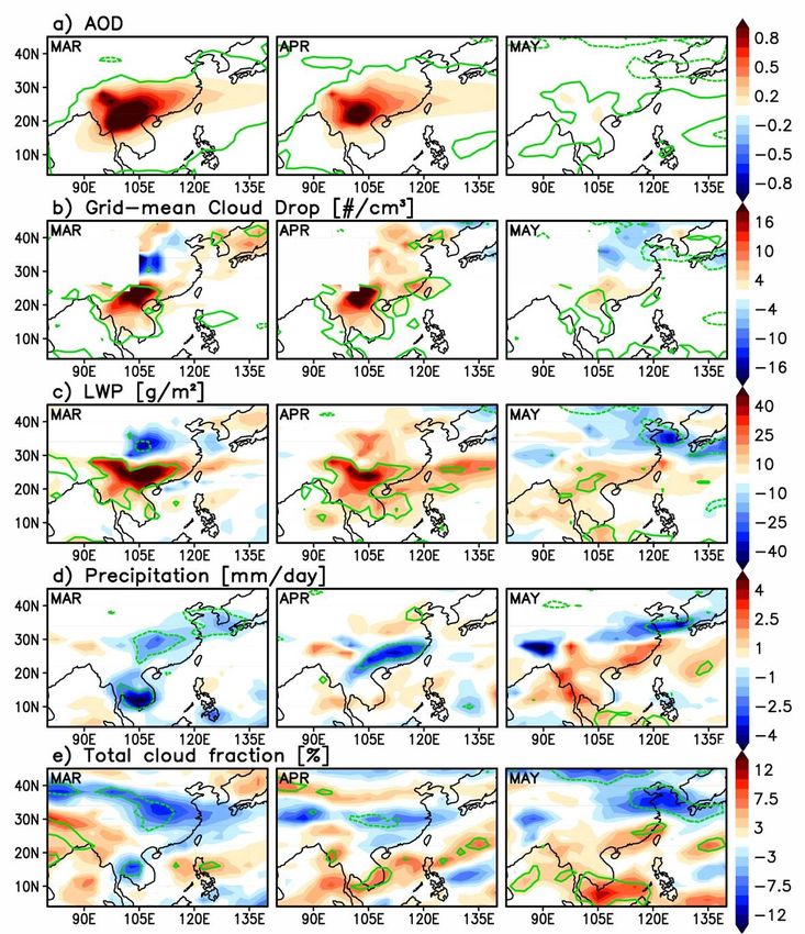
6854                                              D. Lee et al.: Modeling the influences of aerosols on pre-monsoon circulation

Table 1. Experimental designs for our GEOS-5 AGCM simulations.         less wet scavenging of aerosols compared to rainy MJJA. Ac-
“Zero” stands for zero BB emissions over the green dash box region     cordingly, aerosol optical depth and aerosol-activated cloud
of Fig. 1a, “High” for high (year 2007, Fig. 1b) emissions. Symbols    particle numbers are expected to be much larger in FMA than
under aerosol direct effect and indirect effect indicate experiments   MJJA. This is the main reason for focusing this investigation
with (O) and without (X) the effect.                                   of BBA direct and indirect effects on FMA and the transition
                                                                       month of May. Our working hypothesis is that high aerosol
                     BB      Direct effect   Indirect effect
                                                                       number concentration in FMA has a strong influence on the
       HighBoth      High          O               O                   radiative forcing, circulation, and precipitation of the local
       ZeroBoth      Zero          O               O                   and surrounding region. Important factors would be aerosol–
       HighInd       High          X               O                   cloud–radiation interactions. The cloud cover over SEA is
       ZeroInd       Zero          X               O                   generally composed of stratiform, low-altitude clouds asso-
                                                                       ciated with frontal systems that originate in China (Hsu et
                                                                       al., 2003). The major type of precipitation would be warm
                                                                       rainfall in the focused season.
solar radiation, thereby reducing the solar radiation reaching            Direct and indirect effects of aerosols are intrinsically in-
the surface, reducing surface sensible and latent heat fluxes          teractive, and therefore their combined effects can be very
(Ramanathan et al., 2005). Chung and Ramanathan (2006)                 different from their linear sum. Even though the fundamen-
showed the so-called “Atmospheric Brown Cloud” decreases               tal physics of aerosol direct and indirect effects is reasonably
the surface solar radiation flux, which reduces surface evap-          well understood, uncertainty of aerosol data under cloudy
oration while also weakening latitudinal sea surface temper-           conditions and complexities in coupling the aerosol–cloud–
ature (SST) gradients and stabilizing the troposphere, caus-           radiation interactions prohibit a better understanding of the
ing monsoon rainfall decreases. On the other hand, absorp-             impact of these processes. For example, a positive relation-
tion of solar radiation at the aerosol level warms the local           ship between AOD and total cloud cover (TCC) was shown
atmosphere, inducing elevated heating that can invigorate              in satellite data (Kaufman et al., 2005; Kaufman and Koren,
air mass convergence near the surface and, with the addi-              2006), but the dominant contribution to the AOD–TCC re-
tion of sensible and latent heat, can make the PBL unstable            lationship have been attributed to aerosol swelling in humid
enough to promote moist convection (Lau et al., 2006; Lau              air rather than the direct effects of aerosols on the cloud fields
and Kim, 2006, 2014). The net outcome of the resulting com-            (Quass et al., 2010).
plex feedback interactions may either increase or decrease                Aerosol–cloud interaction effects on South Asia to East
local rainfall (Meehl et al., 2008). Furthermore, many par-            Asia circulation and monsoons have been the subject of in-
ticles from BB emission are active cloud condensation nu-              vestigations with regional models (Wu et al., 2013; Lim et
clei (CCN) (Petters et al., 2009). Hence more BB emission              al., 2014) as well as global climate models (Bollasina et
leads to more CCN and ice nuclei (IN) and thereby more                 al., 2011; Ganguly et al., 2012; Guo et al., 2013). Our cur-
cloud particles. If we assume that the net condensate pro-             rent cloud physics scheme, Microphysics of clouds with Re-
duction is solely governed by cloud-scale dynamics, more               laxed Arakawa–Schubert moist convection upgraded with
CCN would imply larger numbers but smaller cloud droplets              prognostic aerosol–cloud interactions (McRAS-AC; Sud et
and thereby an increase in cloud albedo (Twomey, 1977).                al., 2013), has indirect effect simulation capabilities, and has
Smaller cloud particles would also hamper the autoconver-              been implemented in the GEOS-5 AGCM (Rienecker et al.,
sion of cloud water into precipitation, so the presence of BB          2008). It provides an opportunity to perform simulation stud-
sources is expected to reduce the precipitation production             ies to systematically assess the influence of BBA on rainfall
rate and increase cloud lifetime (Albrecht, 1989). However,            and circulation in SEA. Clearly, constrained model simula-
this process is only applicable to warm rain. Observations             tions are one plausible way to better distinguish between the
show that cold and mixed cloud regimes have complicated                roles of direct and indirect effects and their interactive influ-
responses, as summarized in Tao et al. (2012, Table 1). Li et          ences that depend on circulation, cloud types, and aerosol-
al. (2011), with extensive observational analysis in the At-           dependent cloud microphysics. While in principle these ef-
mospheric Radiation Measurement (ARM) site at Southern                 fects can be properly simulated only with a coupled ocean–
Great Plains, show that cloud-top height and thickness in-             atmosphere model, as a first step we use an AGCM with pre-
crease with aerosol concentration in mixed-phase clouds and            scribed monthly SSTs and with aerosol emission anomalies
rain increases with aerosol concentration in deep clouds, but          prescribed from the Quick Fire Emissions Dataset (QFED)
declines in clouds that have low liquid-water content.                 data set (see Sect. 2.1). This way we can isolate the influence
   Satellite data reveal that during FMA, the SEA region ex-           of BBA over land by comparative assessments of circulation
hibits the highest aerosol concentrations, an order of mag-            and rainfall changes in neighboring regions.
nitude greater than that in the summer monsoon May-June-                  In this endeavor, we perform a comprehensive model sim-
July-August (MJJA) season because of more BBA sources                  ulation study with the physically interactive aerosol–cloud–
during dry FMA (Ichoku et al., 2008; Lin et al., 2009) and             radiation treatment of McRAS-AC as implemented in the

Atmos. Chem. Phys., 14, 6853–6866, 2014                                                  www.atmos-chem-phys.net/14/6853/2014/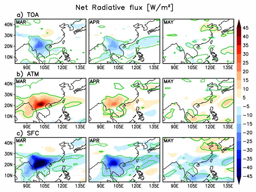
D. Lee et al.: Modeling the influences of aerosols on pre-monsoon circulation                                                 6855

GEOS-5 AGCM, in order to better understand the spatiotem-           tered in a coarse resolution GCM. These algorithms work
poral modulation of the SEA pre-monsoon season by BBA.              seamlessly across widely varying vertical model-layer thick-
Section 2 describes the data set, model and experimental de-        nesses. Any change in the cloud water substance mass by
sign; results and a summary are presented in Sects. 3 and 4,        condensation/deposition and/or collection by precipitation
respectively.                                                       works interactively through an implicit backward numerical
                                                                    integration that approximates the solution of the basic non-
                                                                    linear coupled differential equations for the cloud source and
2     Data, model and experimental design                           sink terms of the mass balance tendency equation. Despite
                                                                    using the observationally based Sundqvist (1988) equations
2.1    Data sets for aerosol effect analysis
                                                                    for the mixed phase and ice phase precipitation tendencies,
BB is a major source of primary emissions of carbonaceous           the implementation of the Barahona and Nenes (2009a, b)
aerosols over the SEA region. QFED (Darmenov and da                 ice nucleation and the Bergeron–Findeisen cloud water-to-
Silva, 2013) was developed to meet the needs of the NASA            ice mass transfer (Rotstayn et al., 2000) allows for a reason-
Goddard Earth Observing System Model (GEOS) with re-                able separation of cloud liquid and ice mass fractions with
gard to atmospheric constituent modeling and data assimila-         their accompanying liquid and ice particle number concen-
tion of BB events. QFED is based on global gridded fire ra-         trations. Homogenous freezing of in-cloud liquid droplets
diative power, derived from the Moderate Resolution Imag-           surviving below −38 ◦ C is enforced by assuming instanta-
ing Spectroradiometer (MODIS) Level 2 fire product. QFED            neous freezing. Aerosol–cloud interactions are implemented
is used not only as a BB inventory for the global Goddard           into both stratiform (large-scale) clouds, and convective tow-
Chemistry Aerosol Radiation and Transport (GOCART, Chin             ers topped by detraining convective anvils that transform
et al., 2002, Colarco et al., 2010) model in the GEOS-5 sys-        into large-scale clouds at a prescribed timescale of an hour.
tem, but also as an index indicating high BB days for our           Sud et al. (2013) provides a much more comprehensive dis-
composite analysis. Version 2.2 used in this study covers the       cussion of McRAS-AC (including treatment of the differ-
period from January 2003 to December 2010. The QFED                 ent cloud types) and its comparative performance against
Level-3 products are available at 0.3125 × 0.25◦ horizontal         the cloud scheme of the baseline model. That study also in-
resolution, but are degraded to 2.5 × 2.0 degree for use in the     cludes sensitivity studies with an interactive aerosol module
present model simulation. The 1◦ MODIS Aqua level 3 daily           and modified aerosol size distribution. The model used in
product (MYD03_D3) is used for aerosol optical depth (Chu           the current study contains all the upgrades outlined above.
et al., 2002) and liquid cloud effective radius (Platnick et al.,   The CFMIP Observation Simulator Package (COSP, http:
2003). The data cover the period from July 2002 to present.         //cfmip.metoffice.com/COSP.html) is also employed online
For precipitation, 1◦ daily Global Precipitation Climatology        in our experiments. Because of the significant differences
Project (GPCP-1DD; Huffman et al., 2001) data are used,             between the way clouds are observed and represented in
covering the period October 1996 to present.                        models, a “satellite simulator” facilitates proper compari-
                                                                    son and validations of the key simulated cloud and radia-
2.2    GEOS-5 AGCM with double moment microphysics                  tion fields against observations (Klein et al., 2013). The GO-
       and updated radiation                                        CART module provides prognostic aerosols fields consist-
                                                                    ing of five aerosol species with fifteen modes. There are five
The numerical model used for this study is the GEOS-                modes of dust and sea salt sorted in different particle size
5 AGCM, version Fortuna 2.5 documented by Molod                     bins; there are two modes of organic and black carbon to sort
et al. (2012). In the current application, McRAS-AC re-             hydrophilic and hydrophobic particles; and one mode of sul-
places the cloud scheme of the baseline model. McRAS-               fate particles. All aerosol modes are assumed to be “exter-
AC synthesizes the initial version of McRAS (described in           nally” mixed. The GOCART module runs interactively and
Sud and Walker, 1999, 2003) with subsequently developed             provides prognostic aerosol fields within the AGCM.
aerosol–cloud interaction microphysics described in Sud and            Accurate radiation calculations are also very important for
Lee (2007). The latest modification to McRAS-AC includes            properly simulating aerosol direct/indirect effect. Our means
the addition of Barahona and Nenes (2009a, b) ice nucle-            of calculating realistic cloud radiative effect (CRE) is the ad-
ation for mixed phase and ice phase clouds, as well as Foun-        vanced RRTMG radiative transfer package (Clough et al.,
toukis and Nenes (2005) liquid droplet formation. The pre-          2005) equipped with a subcolumn generator in the GEOS-
cipitation parameterization remains as before, namely Sud           5 AGCM. RRTMG can be run in Monte Carlo Indepen-
and Lee (2007) for the liquid phase and Sundqvist (1988)            dent Column Approximation (McICA) mode (Pincus et al.,
for the mixed and ice phases. In-cloud evaporation, precip-         2003) that operates on subcolumns with either clear or com-
itation and self-collection of cloud water are parameterized        pletely overcast cloud layers produced by a cloud generator.
according to Sud and Lee (2007), employing a reformu-               Whether the cloud condensate in a particular layer is dif-
lated version of the Seifert and Beheng (2001, 2006) param-         ferent from subcolumn to subcolumn depends on the spe-
eterization to handle the much thicker cloud layers encoun-         cific assumptions about horizontal cloud heterogeneity as

www.atmos-chem-phys.net/14/6853/2014/                                                Atmos. Chem. Phys., 14, 6853–6866, 2014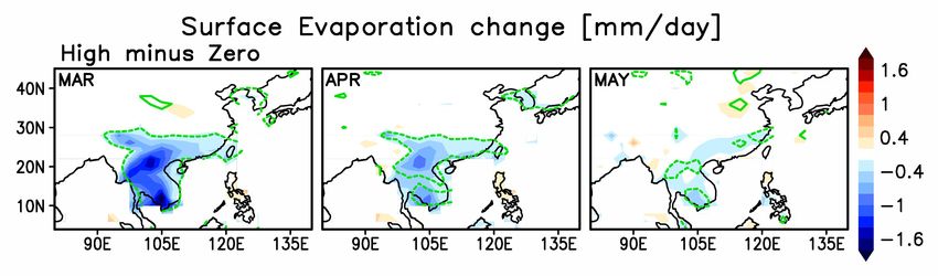
1    Fig. 1. QFED BB emission data (OC data is used for this figure, unit of µg/m2/s). a) February-
            2    March-April mean and b) averaged time series for dashed box area. Time series are smoothed by
            3    a seven-day moving average. Orange line represents data for year 2007 for high BB simulation
6856        4    experiments. Other years are plotted
                                               D. Leeinetgray.
                                                          al.: Modeling the influences of aerosols on pre-monsoon circulation

            5
Figure 1. QFED BB emission data (OC data is used for this figure, unit of µg m−2 s−1 ). (a) February-March-April mean and (b) averaged
             6
time series for dashed box area. Time series are smoothed by a 7-day moving average. Orange line represents data for year 2007 for high BB
simulation experiments. Other years are plotted in gray.

determined by distributions of condensate specified within      sion experiments. Such an “aerosol on” and “aerosol off” de-
the cloud generator. A prior implementation of McRAS-AC         sign is often used in aerosol–climate sensitivity studies (e.g.,
(Sud et al., 2013) used cloud water path scaling to account     Lau et al., 2006; Wu et al., 2013) to better depict the aerosol
for the radiative effects of subgrid scale cloud water inho-    signal, but this methodology has the drawback of making the
mogeneity. More detailed discussions about RRTMG in the         comparison of simulations with observations difficult. Initial
GEOS-5 AGCM can be found in Oreopoulos et al. (2012).           simulation sets using year-to-year emission data set did not
                                                                yield statistically significant differences on circulation, while
2.3 Experimental design                                         some sensitivity to enhanced emissions could be discerned
                                                                in increased AODs, brightened liquid clouds and decreased
In order to investigate BBA effects on SEA climate, sev-        rainfall. Clearly, by design, the differences between “High”
eral observation-inspired experiments with and without BB       and “Zero” emission experiments yield the effect of BBA,
emission over SEA are designed. Figure 1a shows the cli-        black carbon, organic carbon, and sulfate originating from
matological amount of carbonaceous aerosol emission from        the boxed area and in order to isolate statistically significant
BB during FMA averaged over 8 years from 2003 to 2010,          signals a Student’s t test is employed. We considered the dif-
and Fig. 1b depicts the time series of the boxed area. The      ferences exceeding the 95 % confidence level in a difference
QFED data set described earlier was used for this figure.       field as statistically significant.
Massive BB emissions occur during FMA in the eastern re-           The differences between “HighBoth” and “ZeroBoth”
gions of Cambodia, Myanmar, Laos, and northern Thailand         simulations are a measure of the total BB effect. Here,
with peaks in March. Figure 1b shows large temporal vari-       “Both” means that the model’s experimental setup includes
ations of BB emissions. It could be high in one month and 33 both aerosol direct and indirect effects. The indirect-only
also could become near zero in another month.                   simulations are denoted by “HighInd” and “ZeroInd” exper-
   To isolate the potential BBA effects, the AGCM exper-        iments. In these simulations, we neglect the aerosol direct
iments were performed with climatological SSTs to elimi-        effect by turning off aerosol radiative interactions globally,
nate large-scale forcing (e.g., El Niño events) influences due  thereby allowing only the indirect effects of aerosols to op-
to SST variability. Moreover, to separate the signal from       erate on clouds and influence their radiative effects. HighInd
the model’s own internal variability, multi-member ensemble     minus ZeroInd differences therefore measure the strength of
simulations were performed. Each simulation-set consists of     the BBA indirect effect. Finally, while not additive due to
a 10-member ensemble covering the early January to late Au-     nonlinearities, comparing “Both” and “Ind” runs gives in-
gust period; each runs starts with different initial conditions sight into the relative contributions of direct and indirect ef-
taken from the model runs used in Sud et al. (2013). To es-     fects to the total aerosol effect.
timate the signal of aerosol effects on climate variability, we
conducted experiments with “Zero” BB emission over the
green dash box region (Fig. 1a) and compared them to exper-
iments with “High” BB emission in 2007. BB emissions out-
side of the boxed area and all other sources of aerosol were
set to climatological means for both “High” and “Zero” emis-

Atmos. Chem. Phys., 14, 6853–6866, 2014                                                  www.atmos-chem-phys.net/14/6853/2014/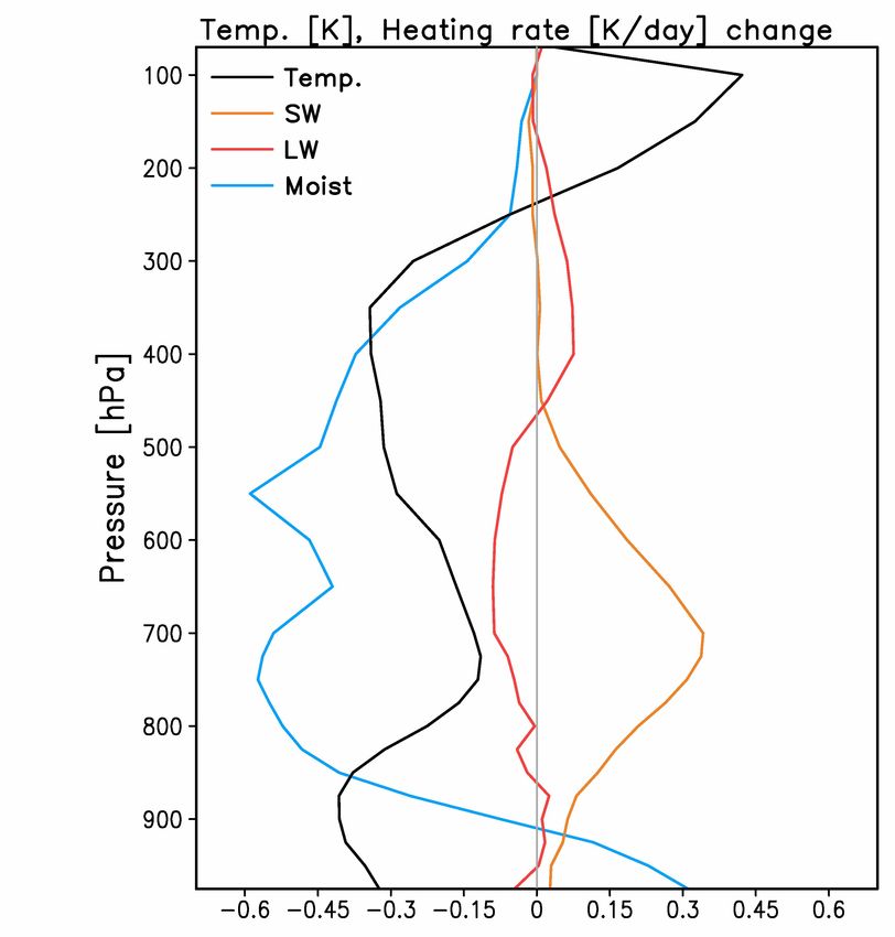
1   Fig. 2. Composite analysis and differences (Diff) in a) aerosol optical depth and b) liquid cloud
                                                                           2   effective radius (µm) from MODIS-Aqua retrievals, and c) GPCP precipitation (mm/day). High
                                                           3  emission (left), climatology (middle) and differences: high minus climatology (right) panels
D. Lee et al.: Modeling the influences of aerosols on pre-monsoon    circulation                                                                   6857
                                                                           4   respectively. Here 36 high emission days and 8-years climatology data are used.

3     Results

3.1    Comparison between model simulations and
       satellite observations

Some insight on the effects of BB in SEA can be obtained
by comparing high and climatological BB conditions in ob-
servations. We have constructed composites of MODIS Aqua
Level 3 daily products (MYD03_D8) for 36 days of the high-
est BB emission index within the 2003 to 2010 period. The
BB emission index is defined as the area average for the
dashed box area in Fig 1a. Smoothed time series of the index
is shown in Fig. 1b. Figure 2 shows comparisons between the
high-emission days and the 8-year climatology of MODIS-                    5

Aqua AOD (Fig. 2a) and liquid cloud effective radius (Reff ,               6    Figure 2. Composite analysis and differences (Diff) in (a) aerosol
Fig. 2b). When BB is high in FMA over inland areas of SEA                       optical depth and (b) liquid cloud effective radius (µm) from
compared to normal days, anomalously high AOD appears                           MODIS-Aqua retrievals, and (c) GPCP precipitation (mm day−1 ).
over the northern part of SEA up to the coast of southern                       High emission (left), climatology (middle) and differences: high mi-
China. According to Lau and Kim (2014), low-level wind                          nus climatology (right) panels respectively. Here 36 high-emission
in the area carries BBA from the source region to southern                      days and 8-year climatology data are used.
China, resulting in the high BB AOD anomaly of Fig. 2a. Ac-
cording to the rightmost panel of Fig. 2b, the corresponding
negative anomaly of Reff coincides with the region where a                      ingly Reff decreases. Not only are McRAS-AC AGCM sim-
positive AOD anomaly exists. This is a classic manifestation                    ulations capable of simulating the response of cloud droplets
of aerosol indirect effect whereby increased BBA reduces                        to AOD, but the model’s overall34    response exhibits reason-
the size of cloud droplets by increasing CCN number con-                        able spatial coherence with the composite maps of observa-
centration. Indeed, if the negative anomaly of Reff is related                  tion data (Fig. 2), particularly on the downwind side of the
to aerosol, then the imprints of other aerosol indirect effects                 BB source. Wind vectors at 800 hPa are plotted on Fig. 3a
may also exist in other meteorological fields, such as the pre-                 to explain an advection of BBA. For precipitation, the obser-
cipitation. Figure 2c compares composited daily GPCP pre-                       vations show a dipole-like anomaly pattern, namely overall
cipitation for the enhanced BB days and the climatology. The                    decrease near source area and at eastern locations, and in-
difference plot reveals a negative precipitation anomaly over                   crease further east near the coast (Fig. 2c, Diff). In the model,
the aerosol source and its adjacent areas while in the vicinity                 on the other hand, the average BB signal on FMA precipita-
of the east coast of China increased rainfall is observed. This                 tion materializes as a reduction in the precipitation of large
can be interpreted in a Lagrangian framework, by the cloud                      areas south and east of the source region. Since SSTs were
holding more cloud water due to reduced autoconversion ef-                      prescribed climatologically, less meaningful responses over
ficiency, but as the cloud advects downwind (i.e., towards the                  the ocean is expected. Potential BBA effects on SEA pre-
northeast direction), it eventually releases cloud water as pre-                monsoon are investigated further in the following sections by
cipitation far away from the source region. Higher BB emis-                     taking appropriate differences of GEOS-5 experimental sets
sion days are selected from every year and compared with                        described earlier.
climatology to remove interannual variability and SST forc-
ing and isolate the BBA effects. However, since large-scale                     3.2     BB effects on cloud microphysics and precipitation
SST forcings, such as El Nino, can simultaneously trigger a                             simulation
reduction in precipitation and an increase in aerosols (Tosca
et al., 2010), it is necessary to study shifts in the precipitation             One of the mechanisms that changes the nature and amount
pattern from AGCM simulations.                                                  of precipitation is cloud microphysical processes as influ-
   In order to evaluate the sensitivity of the AGCM to BBA                      enced by aerosols, widely known as the aerosol second in-
variations, model output is compared to the satellite data                      direct effect (Albrecht, 1989). This mechanism acts on the
analysis. Figure 3 shows the overall BBA-simulated sensi-                       autoconversion rate that modulates the intensity of liquid pre-
tivity of the model as the difference between HighBoth and                      cipitation. Our area of focus where precipitation decreases
ZeroBoth experiments. Anomalies in Reff are obtained using                      in MODIS analysis and model simulations is likely affected
COSP’s MODIS simulator in the GEOS-5 AGCM for fair                              by BBA that are transported to southern China, where a per-
comparison with observations. For the 10-member ensem-                          sistent cloud band exists. In the model simulation the hori-
ble mean, simulated AOD increases downwind (i.e., towards                       zontal and vertical location of aerosol and the cloud band(s)
the northeast direction) of the BB source and correspond-                       are in close proximity, as seen in Fig. 4. The figure shows

www.atmos-chem-phys.net/14/6853/2014/                                                                    Atmos. Chem. Phys., 14, 6853–6866, 2014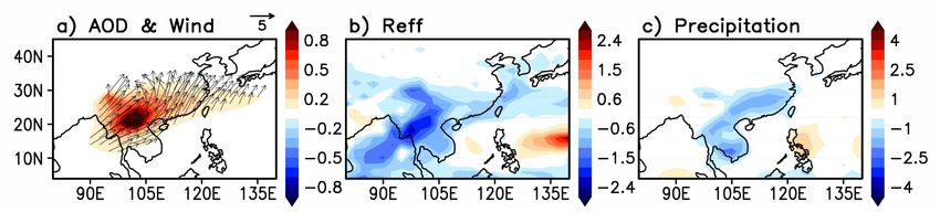
1 Fig. 3. Same variables as in Fig. 2 but for HighBoth minus ZeroBoth differences of AGCM
2 simulations. Panels show a) aerosol optical depth, b) liquid cloud effective radius (µm) and
3 precipitation rate (mm/day) during the FMA time period. Vectors on a) are wind vectors at 800
6858 4 hPa from ‘HighBoth’, only plotted where
D. Lee AOD
et al.: increases.
Modeling the influences of aerosols on pre-monsoon circulation
5
Figure 3. Same variables as in Fig. 2 but for HighBoth minus ZeroBoth differences of AGCM simulations. Panels show (a) aerosol optical
6
1
depth, (b) liquid cloud effective radius (µm) and precipitation rate (mm day−1 ) during the FMA time period. Vectors on (a) are wind vectors
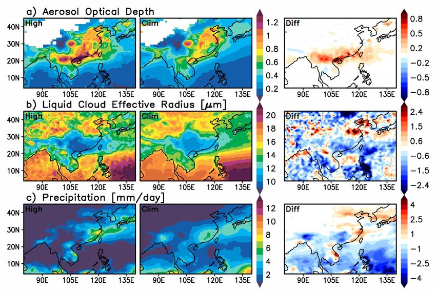
Fig. 4. Vertical cross section of simulated mixing ratio of BBA (shading, µg/kg) and cloud liquid
2
at 800
water hPa from
(contour, mg/kg) HighBoth, only simulations;
in March in HighBoth plotted where AOD increases.
zonal averaging is performed for 105
3 to 120E.
rate process via the parameterization,
∂Lc
= −KL4c Nc−2 , (1)
∂t auto
where Lc is the cloud liquid water content (kg m−3 ), Nc is
the cloud drop number concentration (m−3 ), and K is an ac-
cumulated constant for autoconversion (see Eq. A.2 in Sud
and Lee, 2007, with units of kg−3 m3 s−1 ). From Eq. (1), as
Nc increases under the assumption of constant Lc , the au-
toconversion rate decreases. The occurrence of this second
4 aerosol indirect effect is shown by the model experiments.
5 Figure 4. Vertical cross section of simulated mixing ratio of BBA Monthly mean difference fields between HighBoth and Zer-
(shading, µg kg−1 ) and cloud liquid water (contour, mg kg−1 ) in oBoth experiments from March to May are shown in Fig. 5
March in HighBoth simulations; zonal averaging is performed for for AOD, Nc , cloud liquid water path (LWP), precipitation
105 to 120◦ E. and total cloud fraction. Nc has been vertically averaged from
900 to 750 hPa. Red (blue) color indicates positive (negative)
anomaly with increasing BBA. Green contours delineate the
areas where the change by BBA is significant at the 95 % sig-
the vertical cross section of the BBA mixing ratio (shading) nificance level, based on Student’s t test. Aerosols clearly in-
and cloud liquid water content (contour) for March, obtained crease due to BB emission with an annual peak in March, and
from the HighBoth experiment in the vicinity of decreased so does the AOD anomaly. Since February is a dry season for
precipitation as shown in Fig. 3c (105 to 120◦ E). BBA are the area, the analysis focuses on March, April and May, with
lifted aloft by topography (oriented in a north–south direc- the latter month delineating the onset of the East Asian mon-
tion), and act as an additional source of CCN in pre-existing soon. With BB occurring mainly in early spring, aerosol con-
clouds which are mostly low-level36 (warm) and therefore of centrations in May should not be affected much, so any sig-
liquid phase at this particular location and time of the year. 35 nal in the meteorological fields for that month is potentially
In the model, BB produces sulfate and carbonaceous due to circulation and land surface changes induced by BB
aerosols that can be activated as cloud droplets. Sulfate emissions in the preceding months. In the model we can de-
aerosols are highly soluble, while the carbonaceous aerosols compose AOD anomaly by species. The difference of AOD
have both hydrophobic and hydrophilic modes. Hydrophilic between HighBoth and ZeroBoth experiments over the boxed
organic and black carbon aerosols have prescribed fractions area in Fig. 1 for the month of March is 0.6, 0.487 com-
of soluble mass (0.25 and 0.1) so they also act as CCNs. ing from organic carbon, 0.063 from sulfate, and 0.05 from
Thus BBAs present at the level of developing liquid clouds black carbon. There is some amount of “background” sul-
also activate along with the background aerosols. Under con- fate in ZeroBoth (AOD = 0.129), but organic and black car-
ditions of massive BB, the CCN number concentration in- bon aerosols are mostly from BB emissions, so their AODs
creases greatly, yielding increased cloud drop number con- in ZeroBoth are quite small, 0.031 and 0.013, respectively.
centration and reduced cloud droplet sizes for constant cloud Dust and sea salt aerosol presence are very small over the
water. The underlying physics leading to the reduction in Reff region with AODs less than 0.01.
is well captured by the model (Fig. 3b). Smaller droplets re- As stated earlier, as the BBA loadings increase, grid mean
duce the efficiency of autoconversion from cloud liquid wa- Nc , the product of in-cloud Nc and cloud fraction also in-
ter to rain, resulting in less precipitation. The double mo- creases. Overall, both Nc and LWP increase in the high
ment microphysics in McRAS-AC reduces autoconversion BB experiments due to delayed precipitation, particularly in
Atmos. Chem. Phys., 14, 6853–6866, 2014 www.atmos-chem-phys.net/14/6853/2014/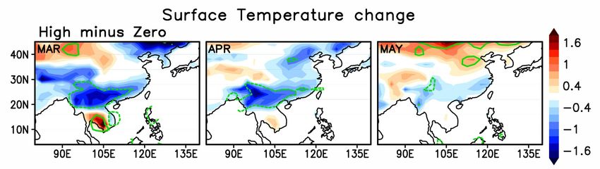
1   Fig. 5. HighBoth minus ZeroBoth representing BBA effects on a) aerosol optical depth, b) grid
2   mean cloud drop number concentration, c) liquid water path (LWP), d) precipitation and e) total
3   cloud fraction (%) from COSP. Green contour mark regions of >95% significant in a student’s t-
    D. Lee et al.: Modeling the influences of aerosols on pre-monsoon circulation                                                                                6859
4   test.

                                                                                                      precipitation is found in May, suggesting that large BB emis-
                                                                                                      sion in March and April can have a delayed effect even in
                                                                                                      regions far away from the source. Microphysical processes
                                                                                                      may therefore not be the only mechanism that reduces pre-
                                                                                                      cipitation. The impact of BBA on May precipitation could be
                                                                                                      a combination of direct, indirect effects, and feedback pro-
                                                                                                      cesses initiated by aerosols in March and April. Further anal-
                                                                                                      ysis of circulation changes is needed to distinguish whether
                                                                                                      this anomaly can be attributed to cloud microphysics or some
                                                                                                      other mechanism, a topic that we will address in Sect. 3.4.

                                                                                                      3.3   BB effects on the radiation budget

                                                                                                      BBA can change the radiation balance by both their direct
                                                                                                      and indirect effects. The direct effect of BBA consists of
                                                                                                      scattering (sulfate aerosols) and absorption (black carbon
                                                                                                      aerosols) of incoming solar radiation which cause surface
                                                                                                      cooling and atmospheric heating. As discussed in Sect. 3.2,
                                                                                                      the indirect effect of BBA comes from altering cloud optical
                                                                                                      properties like Reff and cloud amount which modify the net
                                                                                                      (= shortwave + longwave) radiation budget at the top of the
                                                                                                      atmosphere (TOA), atmosphere (ATM), and surface (SFC).
5
                                                                                                      Figure 6 illustrates the magnitude of the net radiation change
    Figure 5. HighBoth minus ZeroBoth 37     representing BBA effects on                              at TOA, ATM, and SFC due to both direct and indirect
    (a) aerosol optical depth, (b) grid mean cloud drop number con-                                   aerosol effects, primarily due to changes in shortwave (SW)
    centration, (c) liquid water path (LWP), (d) precipitation and (e)                                radiation. Each map shows the monthly mean difference be-
    total cloud fraction (%) from COSP. Green contour mark regions of                                 tween HighBoth and ZeroBoth experiments from March to
    > 95 % significant in a Student’s t test.                                                         May with red (blue) indicating heating (cooling) anomalies
                                                                                                      by aerosol, and green contours delineating the areas of statis-
                                                                                                      tically significant change. The overall net radiative effect of
    March and April. Still, some regions exhibit negative grid                                        BBA is TOA/SFC cooling, and ATM heating near the source
    mean Nc and LWP anomalies, possibly because of reduced                                            region, but its interpretation requires further scrutiny because
    cloud fraction (Fig. 5e) due to reduced grid-scale relative                                       contributions to net radiation change also come from circula-
    humidity (RH) that determines cloud amount for stratiform                                         tion changes and associated feedbacks. The ATM heating in
    clouds. The reduced RH is the outcome of larger stability of                                      March and April provides a clearer signal of direct effects
    the lower atmosphere, which suppress rising motion.                                               since the radiative heating comes almost exclusively from
       While enhanced BB emission increases AOD, CCN, Nc ,                                            aerosol absorption, while TOA and SFC cooling comes from
    and even Lc , the relationship is not linear. Increased Lc                                        both direct and indirect aerosol effects. In May there is little
    eventually creates a tendency for higher autoconversion and                                       aerosol direct effect, but a significant anomaly signal exists at
    precipitation rates, which opposes the tendency of the in-                                        the TOA and SFC due to feedbacks from circulation changes.
    creased Nc (Eq. 1). If we do not account for complex feed-                                        When examining TOA and SFC radiation fields in May, the
    backs, precipitation near the BB emission source can be                                           dipole pattern seen near the east coast of China and Korea
    expected to decrease if the increased Nc effect is stronger                                       is due to cloud fraction change (Fig. 5e) consistent with the
    than the enhanced Lc effect, as shown in Fig. 5d for March                                        precipitation change shown in Fig. 5d, and discussed further
    and April. While the satellite data analysis suggests alternat-                                   in the following section.
    ing negative-positive precipitation anomalies along the wind                                         Table 2 shows the differences between HighBoth and Ze-
    flow, a weak positive anomaly surrounds the simulated strong                                      roBoth experiments of the net downward (down minus up)
    negative anomaly over the South China Sea and northern                                            fluxes in March when BBA peaks, regionally averaged across
    China in April (Fig. 5d). This may be explained by two                                            the emission control region. Aerosol radiative effects are
    possible mechanisms. Liquid cloud water gets transported                                          much larger in the SW than the longwave (LW), so most of
    downstream instead of precipitating out locally because of                                        the net radiation change comes from SW effects. The cor-
    suppressed autoconversion, while reduced local precipita-                                         responding clear sky fluxes demonstrate that BBA increases
    tion creates favorable circulation conditions for precipitation                                   SW reflectance, but also absorbance, because large fractions
    downwind. Meanwhile, a statistically significant anomaly of                                       of BBA are composed by carbonaceous aerosols, which are

    www.atmos-chem-phys.net/14/6853/2014/                                                                              Atmos. Chem. Phys., 14, 6853–6866, 2014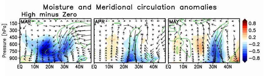
1   Fig. 6. Same layout as in Fig. 5, but for net radiative fluxes at a) top of the atmosphere, b)
    6860                                                                 D. Lee et al.: Modeling the influences of aerosols on pre-monsoon circulation
2   column atmosphere, and c) surface.

                                                                                                     perature anomaly due to BBA is plotted in Fig. 7 and can be
                                                                                                     seen to be very significant near the source region in March
                                                                                                     and April. Weak negative anomalies also appear in May,
                                                                                                     but are mostly insignificant statistically. The vertical profile
                                                                                                     of temperature change (black line) by BB, regionally aver-
                                                                                                     aged from 100 to 120◦ E and from 18 to 30◦ N (cf. red box
                                                                                                     in Fig. 7), is plotted in Fig. 8. This profile is obtained as
                                                                                                     the difference between the HighBoth and ZeroBoth exper-
                                                                                                     iments in March and April when the decrease of precipi-
                                                                                                     tation is significant, and reveals the presence of a cooling
                                                                                                     signal from the surface all the way up to the 250 hPa level.
                                                                                                     In order to better understand what causes the temperature
                                                                                                     change, the model’s major heating/cooling rate contributions
                                                                                                     are shown in Fig. 8. The orange line shows the SW heat-
3
                                                                                                     ing rate (K day−1 ) anomaly, the red line the LW heating rate
                                                                                                     anomaly, and the blue line the anomaly of the heating rate
4   Figure 6. Same layout as in Fig. 5, but for net radiative fluxes at (a)                          due to the model’s moist physics, namely large-scale con-
    top of the atmosphere, (b) column atmosphere, and (c) surface.
                                                                                                     densation and convective processes. As expected, SW radi-
                                                                                                     ation heats the atmosphere near the height of the aerosol
    Table 2. Radiative flux change (W m−2 ) by BBA: numbers indi-                                    layer (Fig. 4). The reason the temperature profile does not
    cate the difference between HighBoth and ZeroBoth experiments in                                 cross over to the positive side is due to other contributors to
    March and April, regionally averaged from 90 to 110◦ E and from                                  temperature change, namely LW and moist physics, both of
    12 to 30◦ N only including land grid (emission control region). All                              which cool the low and middle troposphere. The increase in
    fluxes are net downward, which means upward fluxes are subtracted
                                                                                                     LW cooling is a consequence of increased cloud liquid water
    from downward fluxes.
                                                                                                     between 800 to 600 hPa due to aerosol-induced changes in
                                              TOA         ATM           SFC                          cloud microphysical processes. Although the magnitude of
                                                 38                                                  LW cooling is only about a quarter of the SW heating, it has
                      SW, all sky             −9.5        15.1        −24.6                          an impact since LW cooling occurs at the time and location
                      SW, clear sky           −9.0        17.1        −26.1                          of SW heating, because of liquid water and BBA collocation.
                      LW, all sky              0.3        −2.5          2.8
                                                                                                        The major factor contributing to the negative temperature
                      LW, clear sky            1.2        −1.0          2.2
                                                                                                     anomaly is the reduced moist heating, the most significant
                                                                                                     change of all the heating rate components of the model’s
                                                                                                     physics. A negative moist physics heating rate anomaly
    efficient absorbers of SW radiation. CRE is defined as                                           translates to subdued cloud formation by large-scale con-
                                                                                                     densation and even moist convection. In the area of interest,
    CRE = Fall− sky − Fclear−sky ,                                                           (2)
                                                                                                     March precipitation mostly comes from large-scale conden-
    where F is the net downward flux at the TOA or surface.                                          sation, while in April there is some contribution from moist
    The SW CRE change by BBA (the difference between all                                             convection. The reduced convective precipitation in April,
    sky and clear sky in Table 2 – not shown) is, somewhat sur-                                      accounting for about 40 % of the total precipitation reduc-
    prisingly, positive at the surface (weaker SW CRE for the                                        tion, can be explained by changes in the vertical tempera-
    HighBoth experiment). Despite LWP increases (Fig. 5c) and                                        ture gradient. BBA direct radiative effects make the surface
    Reff decreases (Fig. 3b) in conditions of high BB, yielding                                      cooler and the 700 hPa level warmer, thus decreasing low-
    an average optical thickness increase of 46 % for the cloudy                                     level atmospheric instability as seen in the vertical temper-
    part of the BBA source region, decreased total cloud frac-                                       ature profile anomaly; even though the overall temperature
    tion (Fig. 5e) due to circulation changes overcomes increased                                    change is negative (cooling), a bump of temperature anomaly
    cloud brightness. So, the total indirect effect, namely Reff de-                                 forms near 700 hPa that suppresses the onset of moist con-
    creases (classic “Twomey effect”), accompanying LWP in-                                          vection.
    creases and any resulting cloud feedbacks, seem to counter-                                         Another important reason behind moist physics suppres-
    act the direct aerosol effect in these GEOS-5 experiments.                                       sion, which can explain both large-scale condensation and
                                                                                                     moist convection, is change in atmospheric moisture con-
    3.4     Temperature, moisture, and circulation changes                                           tent. Zonally averaged moisture and meridional circulation
                                                                                                     anomalies due to BBA within 100–120◦ E for March and
    In this section we discuss meteorological the consequences                                       April, and 110–140◦ E for May are plotted in Fig. 9. The
    of the BBA radiative effects, which we have shown to lead to                                     blue shading, indicating dry anomaly, spreads over the 20–
    surface cooling and atmospheric heating. The surface tem-                                        30◦ N latitude zone where the BBA sources are located. A

    Atmos. Chem. Phys., 14, 6853–6866, 2014                                                                           www.atmos-chem-phys.net/14/6853/2014/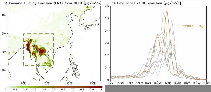
1       Fig. 7. Same layout as in Fig. 5, but for surface temperature (K). Red dashed domain is for area
                    average fields
               2 Modeling
     D. Lee et al.:                in Fig. 8 and
                              the influences  of Table 4. on pre-monsoon circulation
                                                 aerosols                                                                                                       6861

1   Fig. 8. Vertical profile of temperature (K) and heating rate (K/day) differences between
2                   3 simulations for March and April when decrease of precipitation is
    HighBoth and ZeroBoth
3   significant, averaging region 100° E to120° E and 18° N to 30° N and is marked in Fig. 7. Black,
     Figure 7. Same layout as in Fig. 5, but for surface temperature (K). Red dashed domain is for area-averaged fields in Fig. 8 and Table 4.
4                     4 lines represent temperature, SW heating rate, LW heating rate, and the
    orange, red and blue
5   heating rate due to the model’s moist physics.

                       5                                                                               reduced autoconversion leaves behind more in-cloud water,
                                                                                                       which advects downwind instead of being converted into lo-
                                                                                                       cal precipitation, resulting in a reduced supply of moisture
                                                                                                       to the levels underneath and creating a feedback loop where
                                                                                                       weaker latent heat flux at the surface causes further decreases
                                                                                                       in precipitation.
                                                                                                          Several mechanisms can potentially reduce precipitation
                                                                                                       in the downwind side of an active BB region. Cloud micro-
                                                                                                       physics can delay the precipitation process by slowing down
                                                                                                       autoconversion, and then radiation can help make the area
                                                                                                       stable and dry, all conditions unfavorable for vigorous moist
                                                                                                       processes. Moreover, dry anomalies can be the result of cloud
                                                                                                       microphysics as well as in lack of rain and its evaporation.
                                                                                                       Likewise, a number of other variables may be changing in
                                                                                                       the same direction due to direct BBA effects on radiation
                                                                                                       and the indirect effects on cloud microphysics. Both effects
                                                                                                       cause SW dimming at the surface, low-level drying, and de-
                                                                                                       creased precipitation. Separating microphysical from radia-
                                                                                                       tive effects is thus a worthwhile objective which we pursue
6                                                                                                      in the following section.
7    Figure 8. Vertical profile of temperature (K) and heating rate
     (K day−1 ) differences between HighBoth and ZeroBoth simulations                                  3.5   Quantitative breakdowns of direct and indirect
                                   40
     for March and April when precipitation decrease is significant; the                                     effects
     averaging region is 100 to 120◦ E and 18 to 30◦ N and is marked
                                                                      In the previous sections, all the results explaining aerosol ef-
     in Fig. 7. Black, orange, red and blue lines represent temperature,
     SW heating rate, LW heating rate, and the heating rate due to thefects were based on HighBoth and ZeroBoth experiments,
     model’s moist physics, respectively.                             the first including BBA from a high-emission year and the
                                                                      latter entirely neglecting BBA emissions from the area of
                                                                      strongest fire activity. The GEOS-5 AGCM accounted for
     few factors play a role in making this region drier. One is 39 both direct effects in its radiative transfer routines and in-
     reduced surface evaporation (Fig. 10) in the region of neg-      direct effects in its cloud microphysics routines. Differences
     ative surface temperature anomaly. The other is circulation      between the two experiments capture both aerosol direct and
     changes, specifically the substantial downward and south-        indirect effects (as well as feedbacks), in other words, com-
     ward flow anomalies induced by BBA. While the down-              bined effects (CE). In two other experimental sets, the ‘High-
     ward anomaly could be the result of reduced moist activ-         Ind’ and ZeroInd experiments, direct effects of aerosol on
     ity, the accompanying southward anomaly may actually be          radiation are ignored (globally), leaving only the indirect ef-
     the cause of reduced moisture transport from low latitudes.      fect (IE) of BBA to be diagnosed as the difference between
     The column-integrated moisture convergence anomaly (not          the two Ind experiments. Our diagnostic approach to sepa-
     shown) in the region where precipitation decreases is nega-      rate the direct and indirect aerosol effects of a rather complex
     tive with some degree of statistical significance, albeit less   regional climatic response consists of comparing key vari-
     than surface evaporation (Fig. 10). Another possible cause       ables from “CE” and “IE” differences, both including feed-
     for overall drying is the decreased precipitation itself, imply- back from circulation changes.
     ing positive feedback. Because of the BBA indirect effect,

     www.atmos-chem-phys.net/14/6853/2014/                                                                              Atmos. Chem. Phys., 14, 6853–6866, 2014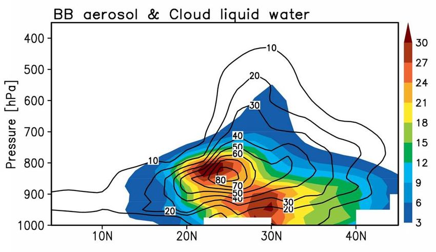
2    (vectors, horizontal component is for meridional wind anomaly, vertical component is for
            3    pressure velocity) from HighBoth minus ZeroBoth experiments over the longitude sector 100–
            4    120° E for March, April and sector 110–140° E for May. Units of pressure velocity, meridional
                                                          -2
6862        5    wind, and water vapor mixingD.
                                              ratio
                                                Leeare
                                                    et 10
                                                       al.: Pa/s, m/s, and
                                                             Modeling   theg/kg respectively.
                                                                            influences of aerosols on pre-monsoon circulation

            6
Figure 9. Zonally averaged profiles of moisture (shading) and meridional circulation anomalies (vectors, horizontal component is for merid-
ional wind anomaly,
            7         vertical component is for pressure velocity) from HighBoth minus ZeroBoth experiments over the longitude sector
100–120◦ E for March and April, and sector 110–140◦ E for May. Units of pressure velocity, meridional wind, and water vapor mixing ratio
are 10−2 Pa1s−1 ,Fig. 10.
                  m s−1    Similar
                        , and      to, Fig.
                              g kg−1        5, but for surface evaporation (mm/day).
                                       respectively.

           2
Figure 10. Similar to Fig. 5, but for surface evaporation (mm day−1 ).
           3

   Table 3 shows the radiative fluxes in the same way as Ta-     Table 3. Radiative flux change (W m−2 ) by indirect effect of BBA,
ble 2, but for “IE” and “CE minus IE”. Evidently, CE of TOA      and the differences from Table 2. “IE” indicates the difference be-
and SFC SW fluxes and atmospheric column SW absorption           tween HighInd and ZeroInd experiments, “CE” indicates the differ-
are much larger than the corresponding IE of aerosols on SW.     ence between HighBoth and ZeroBoth experiments, while the oth-
This implies a much stronger contribution of the direct effect   ers are the same as Table 2.
(DE) of BBA in CE and makes sense because BBAs have
                                                                                         TOA            ATM               SFC
large AOD over the high-emission regions. Moreover, BBA
effects on radiation in the CE runs are quite similar for clear-                       IE  CE-IE      IE   CE-IE       IE   CE-IE
sky and all-sky conditions, as pointed out earlier in Sect. 3.3.    SW,  all sky      0.5     −10    0.0     15.1     0.5   −25.1
                                                                    SW, clear sky −0.3       −8.7 −0.3       17.4     0.0 −26.1
This provides further support for the notion that the IE due        LW, all sky     −2.1       2.4   0.8    −3.3 −1.3          4.1
to BBA is an order of magnitude smaller on the SW and net 41        LW, clear sky −0.4         1.6   0.7    −1.7 −1.1          3.3
radiation compared to the corresponding DE of aerosols as a
component of CE. Net radiation change by IE turns out small
because it depends on both cloud fraction (which depends
on cloud production, cloud dissipation, and cloud advective      ages of these CE and IE breakdowns. While the CE pre-
tendencies) and cloud optical thickness (which depends on        cipitation reduction in HighBoth minus ZeroBoth BBA is
CCN and cloud water removal by precipitation). In ZeroInd,       1.08 mm day−1 , the corresponding IE precipitation reduction
the (BBA-independent) cloud fraction increases while the         is 0.77 mm day−1 only. For a linear system, one would at-
cloud optical thickness decreases compared to HighInd sim-       tribute the 0.31 mm day−1 reduction corresponding to the CE
ulations.                                                        minus IE difference, to the direct aerosol effect, but we are
   One of the interesting features of the BBA signal is de-      well aware that linearity is not necessarily a good assump-
creased precipitation over the downwind side of the source.      tion, so we view the differences as representing add-on di-
The separation of “CE” and “IE” impacts on precipitation         rect effects that also contain effects of interactive circulation
would be interesting to study for this area. To minimize         changes. Even though the IE averages do not show much
feedback contributions, we focus on variables that are pri-      change in the simulated surface temperature and evapora-
marily forced directly during the March and April time           tion of the boxed region, IE does have a prominent role in
frame and near the source region, in particular 100 to 120◦ E    decreasing surface precipitation, which is caused not only by
and 18 to 30◦ N. Table 4 provides the spatiotemporal aver-       autoconversion reduction, but also by low-level drying due to
                                                                 SW dimming in cloudy areas. In other words, the suppressed

                                                                    42
Atmos. Chem. Phys., 14, 6853–6866, 2014                                                   www.atmos-chem-phys.net/14/6853/2014/
1 Fig. 11. Zonal mean temperature (K) and wind (m/s) differences between HighBoth and Zero
2 Both BBA for 110–140E in May. Green contour identifies regions with >95% significant
3 differences according to the Student’s t-test. Black contour on b) is zonal mean wind in
‘HighBoth’ run. circulation
D. Lee et al.: Modeling the influences of aerosols 4on pre-monsoon 6863
Table 4. Analysis of combined effects (CE, Direct+Indirect) and
only indirect effect (IE).
Aerosol Combined Indirect
effect effect effect
Precipitationa (mm day−1 ) −1.08 −0.77
Surface temperaturea (K) −0.59 0.09
Surface evaporationa (mm day−1 ) −0.25 0.07
Moistureb (g kg−1 ) −0.38 −0.23
5
Moist heating rateb (K day−1 ) −0.29 −0.16
Figure 11. Zonal mean temperature (K) and wind (m s−1 ) differ-
Temperatureb (K) −0.24 6
−0.07
ences between HighBoth and Zero Both BBA for 110–140◦ E in
a Regional average from 100 to 120◦ E and 18 to 30◦ N, on March and April,
7 May. Green contour identifies regions with > 95 % significant dif-
and b 975 to 500 hPa vertical. ferences according to the Student’s t test. Black contour on (b) is
8 zonal mean wind in HighBoth run.
autoconversion that follows CCN and Nc increases9 due to
the presence of additional BBA in the IE simulations and
decreases precipitation, which creates a dry anomaly in the cloud interaction (the indirect effect), the drying of the lower
atmosphere beneath the precipitating cloud due to reduced and middle troposphere is caused by both.
evaporation of rain. In comparison, the DE as a part of CE An interesting, and somewhat unexpected, consequence of
has a more straightforward effect on the moisture supply that enhanced BBAs is the May precipitation anomaly near the
can be traced to atmospheric stabilization and reduced sur- Korean peninsula shown in Fig. 5d. Since BB is not a ma-
face temperature due to surface cooling. So while both CE jor factor in May aerosol loadings, the precipitation anomaly
and IE tend to reduce precipitation, the mechanisms can dif- could be due to circulation and land surface changes trig-
fer overall, despite sharing the common processes of slower gered by BB in the preceding month. In March and April, the
autoconversion and low-level drying. surface temperature over Southeast Asia drops significantly
due to the combined direct and indirect solar dimming effect
of BBA and this reduces the meridional temperature gradient.
Figure 9 shows that the overall circulation anomaly heads
4 Summary and discussion south in March and April. The May circulation anomaly ex-
hibits downward motion at 30◦ N and a little upward motion
An aerosol impact study including both the direct and in- south of 30◦ N. According to Kim et al. (2007) an upper level
43
direct effects focusing on the Southeast Asia pre-monsoon jet stream change can induce secondary circulation changes
season is conducted based on simulations using the GEOS- near the entrance of the jet core in East Asia. In their analysis,
5 AGCM with double moment cloud microphysics called an initial surface cooling by the direct effect of sulfate aerosol
McRAS-AC, interactive GOCART aerosol model, advanced results in a reduced north–south thermal gradient. Figure 11a
radiative transfer package RRTMG applying the Monte Carlo shows a similar weakened meridional temperature gradient
Independent Column Approximation, and the CFMIP Obser- change due to surface cooling found in March and April.
vation Simulator Package (COSP). Analysis of GEOS-5 in- This reduced gradient weakens the zonal wind shear through
tegrations with and without BB emission allows us to sepa- the thermal wind relationship, and slows down the westerly
rate the responses of clouds and precipitation to aerosol from jet stream (Fig. 11b). The deceleration causes ageostrophic
those due to changes in meteorological fields. Our analysis meridional winds and, in this case, anomalous sinking mo-
indicates that plausible reasons for the reduced precipitation tion at 30◦ N (see Fig. 9, May), conditions that are less favor-
are (a) vertical stabilization by atmospheric heating aloft ac- able for precipitation. Although Kim et al. (2007) account
companied by surface cooling due to the shortwave scattering only for direct forcing of aerosol, the circulation anomalies
and absorption by the BBA; (b) less efficient autoconversion induced by the BBA emissions of this study are similar, be-
despite liquid water increases due to increased cloud droplet cause indirect effects did not affect much the surface forcing
number concentration; and (c) suppressed moist processes in CE simulations.
due to atmospheric drying. With properly designed experi- While this study provided some confirmation that our BB
ments we managed to separate the impacts of direct and in- sensitivity in the model looks similar to that from the MODIS
direct effects. While vertical stabilization is traced to direct analysis, the “Zero” BB assumption is admittedly extreme.
aerosol–radiation interaction, which causes rapid cloud ad- So the year-to-year change of meteorological fields by BBA
justments (commonly referred to as the “semi-direct effect”) could be weaker than suggested by the results shown here.
because of depressed dynamical forcing, and the reduced But given the plausibility of how the model’s mechanisms
autoconversion rate is primarily a consequence of aerosol– operate, there is good possibility that real conditions would
www.atmos-chem-phys.net/14/6853/2014/ Atmos. Chem. Phys., 14, 6853–6866, 20146864 D. Lee et al.: Modeling the influences of aerosols on pre-monsoon circulation
be consistent with the overall tendencies of the model. Still, Chu, D., Kaufman, Y., Ichoku, C., Remer, L., Tanre, D., and Hol-
there is much room for further development of the GEOS-5 ben, B.: Validation of MODIS aerosol optical depth retrieval over
model towards more realism. For example, phenomena such land, Geophy. Res. Lett., 29, 1617, doi:10.1029/2001GL013205,
as aerosol-induced convective invigoration (Rosenfeld et al., 2002.
2008) cannot be properly reproduced in our model because Chung, C. and Ramanathan, V.: Weakening of North Indian SST
gradients and the monsoon rainfall in India and the Sahel, J. Cli-
heat release due to freezing does not affect the convective
mate, 19, 2036–2045, doi:10.1175/JCLI3820.1, 2006.
mass flux. This process could be better represented in a bulk Clough, S., Shephard, M., Mlawer, E., Delamere, J., Iacono, M.,
mass flux convection scheme (e.g., Kim and Kang 2012), but Cady-Pereira, K., Boukabara, S., and Brown, P.: Atmospheric
it remains to be seen whether its inclusion in such a scheme radiative transfer modeling: a summary of the AER codes, J.
would ultimately affect overall convective activity in a sub- Quant. Spec. Ra., 91, 233–244, doi:10.1016/j.jqsrt.2004.05.058,
stantial way. Evidently, further refinements and cloud model 2005.
validations are needed for a better understanding of the role Colarco, P., da Silva, A., Chin, M., and Diehl, T.: Online
of aerosol–convection interactions in the seasonal develop- simulations of global aerosol distributions in the NASA
ment of the summer monsoon. Our method of separating di- GEOS-4 model and comparisons to satellite and ground-based
rect and indirect aerosol effects may be imperfect, but no bet- aerosol optical depth, J. Geophys. Res.-Atmos., 115, D14207,
ter alternative currently exists given present modeling limita- doi:10.1029/2009JD012820, 2010.
Darmenov, A. and da Silva, A.: The Quick Fire Emissions Dataset
tions. Regardless, we believe that this study provides a foun-
(QFED) – Documentation of versions 2.1, 2.2 and 2.4., NASA
dation on which to develop better methodologies to properly Technical Report Series on Global Modeling and Data Assimila-
distinguish direct and indirect effect sensitivity to aerosols in tion, NASA TM-2013-104606, Vol. 32, 183 pp., 2013.
large-scale models. Fountoukis, C. and Nenes, A.: Continued development of
a cloud droplet formation parameterization for global
climate models, J. Geophys. Res.-Atmos., 110, D11212,
Acknowledgements. Funding from NASA’s Modeling Analysis doi:10.1029/2004JD005591, 2005
and Prediction (MAP) program managed by D. Considine, and Ganguly, D., Rasch, P., Wang, H., and Yoon, J.: Climate
from the Interdisciplinary Research in Earth Science (IDS) response of the South Asian monsoon system to anthro-
program (Water and Energy Cycle Impacts of Biomass Burning pogenic aerosols, J. Geophys. Res.-Atmos., 117, D13209,
subelement) managed by Hal Maring is gratefully acknowledged. doi:10.1029/2012JD017508, 2012.
I.-S. Kang was supported by the National Research Foundation Gautam, R., Hsu, N., Eck, T., Holben, B., Janjai, S., Jantarach,
of Korea (NRF) grant funded by the Korean government (MEST) T., Tsay, S., and Lau, W.: Characterization of aerosols over the
(NRF-2012M1A2A2671775) and the BK21 program. Indochina peninsula from satellite-surface observations during
biomass burning pre-monsoon season, Atmos. Environ., 78, 51–
Edited by: J. Ma 59, doi:10.1016/j.atmosenv.2012.05.038, 2013.
Guo, L., Highwood, E. J., Shaffrey, L. C., and Turner, A. G.: The
effect of regional changes in anthropogenic aerosols on rainfall
of the East Asian Summer Monsoon, Atmos. Chem. Phys., 13,
References 1521–1534, doi:10.5194/acp-13-1521-2013, 2013.
Huffman, G., Adler, R., Morrissey, M., Bolvin, D., Curtis, S.,
Albrecht, B.: Aerosols, Cloud Microphysics, and Joyce, R., McGavock, B., and Susskind, J.: Global precipi-
Fractional Cloudiness, Science, 245, 1227–1230, tation at one-degree daily resolution from multisatellite ob-
doi:10.1126/science.245.4923.1227, 1989. servations, J. Hydrometeorol., 2, 36–50, doi:10.1175/1525-
Barahona, D. and Nenes, A.: Parameterizing the competition be- 7541(2001)0022.0.CO;2, 2001.
tween homogeneous and heterogeneous freezing in cirrus cloud Ichoku, C., Giglio, L., Wooster, M., and Remer, L.: Global char-
formation – monodisperse ice nuclei, Atmos. Chem. Phys., 9, acterization of biomass-burning patterns using satellite mea-
369–381, doi:10.5194/acp-9-369-2009, 2009a. surements of fire radiative energy, Remote Sens. Environ., 112,
Barahona, D. and Nenes, A.: Parameterizing the competition be- 2950–2962, doi:10.1016/j.rse.2008.02.009, 2008.
tween homogeneous and heterogeneous freezing in ice cloud for- Kaufman, Y. and Koren, I.: Smoke and pollution
mation – polydisperse ice nuclei, Atmos. Chem. Phys., 9, 5933– aerosol effect on cloud cover, Science, 313, 655–658,
5948, doi:10.5194/acp-9-5933-2009, 2009b. doi:10.1126/science.1126232, 2006.
Bollasina, M., Ming, Y., and Ramaswamy, V.: Anthropogenic Kaufman, Y., Koren, I., Remer, L., Rosenfeld, D., and Rudich, Y.:
Aerosols and the Weakening of the South Asian Summer The effect of smoke, dust, and pollution aerosol on shallow cloud
Monsoon, Science, 334, 502–505, doi:10.1126/science.1204994, development over the Atlantic Ocean, P. Natl. Acad. Sci. USA,
2011. 102, 11207–11212, doi:10.1073/pnas.0505191102, 2005.
Chin, M., Ginoux, P., Kinne, S., Torres, O., Holben, B., Dun- Kim, D. and Kang, I.-S.: A bulk mass flux convection scheme for
can, B., Martin, R., Logan, J., Higurashi, A., and Nakajima, climate model: description and moisture sensitivity, Clim. Dy-
T.: Tropospheric aerosol optical thickness from the GOCART nam., 38, 411–429, doi:10.1007/s00382-010-0972-2, 2012.
model and comparisons with satellite and Sun photometer Kim, M.-K., Lau, K.-M., Kim, K.-M., and Lee, W.: A GCM study
measurements, J. Atmos. Sci., 59, 461–483, doi:10.1175/1520- of effects of radiative forcing of sulfate aerosol on large scale cir-
0469(2002)0592.0.CO;2, 2002.
Atmos. Chem. Phys., 14, 6853–6866, 2014 www.atmos-chem-phys.net/14/6853/2014/You can also read