A cross-scale study for compound flooding processes during Hurricane Florence
←
→
Page content transcription
If your browser does not render page correctly, please read the page content below
Nat. Hazards Earth Syst. Sci., 21, 1703–1719, 2021
https://doi.org/10.5194/nhess-21-1703-2021
© Author(s) 2021. This work is distributed under
the Creative Commons Attribution 4.0 License.

A cross-scale study for compound flooding
processes during Hurricane Florence
Fei Ye1 , Wei Huang1 , Yinglong J. Zhang1 , Saeed Moghimi2 , Edward Myers2 , Shachak Pe’eri2 , and Hao-Cheng Yu1
1 VirginiaInstitute of Marine Science, College of William & Mary, Gloucester Point, 23062, USA
2 NOAA   National Ocean Service, Silver Spring, 20910, USA

Correspondence: Fei Ye (feiye@vims.edu) and Yinglong J. Zhang (yjzhang@vims.edu)

Received: 24 November 2020 – Discussion started: 8 December 2020
Revised: 27 April 2021 – Accepted: 28 April 2021 – Published: 2 June 2021

Abstract. We study the compound flooding processes that            flooding highlights one of the major pitfalls of the current
occurred in Hurricane Florence (2018), which was accompa-          hurricane intensity scale, which is entirely based on wind
nied by heavy precipitation, using a 3D creek-to-ocean hy-         speed, leaving the potential rainfall and flooding impacts to
drodynamic model. We examine the important role played             be glossed over in initial forecasts that emphasize hurricane
by barrier islands in the observed compound surges in the          category. The record-setting 2020 Atlantic hurricane season
coastal watershed. Locally very high resolution is used in         (which had several very wet storms) highlights the urgency
some watershed areas in order to resolve small features that       and exposes the current knowledge gap for understanding
turn out to be critical for capturing the observed high water      compound flooding processes.
marks locally. The wave effects are found to be significant           A recent example for compound flood events is Hurricane
near barrier islands and have contributed to some observed         Florence that impacted a large area of North Carolina (NC)
over-toppings and breaches. Results from sensitivity tests ap-     in September 2018. Hurricane Florence was the first major
plying each of the three major forcing factors (oceanic, flu-      hurricane of the 2018 Atlantic hurricane season. Originating
vial, and pluvial) separately are succinctly summarized in a       from a strong tropical wave near Cape Verde, west Africa,
“dominance map” that highlights significant compound ef-           it acquired tropical storm strength on 1 September, followed
fects in most of the affected coastal watersheds, estuaries,       by a rapid intensification to a category 4 status on 4 Septem-
and back bays behind the barrier islands. Operational fore-        ber, with estimated maximum sustained winds of 130 mph
casts based on the current model are being set up at NOAA          (58 m s−1 ), and eventually reaching its maximum strength on
to help coastal resource and emergency managers with disas-        11 September. It made landfall south of Wrightsville Beach
ter planning and mitigation efforts.                               near the border between NC and South Carolina (SC) as a
                                                                   category 1 hurricane on 14 September. The slow motion of
                                                                   the storm after the landfall brought heavy rainfall through-
                                                                   out the Carolinas for several days. Compounded by the storm
1   Introduction                                                   surge, the rainfall caused widespread flooding along a large
                                                                   swath of the NC coast and inland flooding in cities such
Recently, more frequent occurrences of “wet” hurricanes            as Fayetteville, Smithfield, Lumberton, Durham, and Chapel
(i.e., hurricanes accompanied by heavy precipitation) that         Hill. According to a USGS report (Fester et al., 2018), a
stall near the coast (Pfahl et al., 2017; Hall and Kossin, 2019)   new record rainfall total of 35.93 in. (0.91 m) was set dur-
have brought new challenges to coastal communities in the          ing the hurricane in Elizabethtown, NC. Many other loca-
form of compound flooding, which is defined as concurrence         tions throughout NC and SC also set new rainfall records
of flooding from the same or different origins (river, storm       (Fig. 1). Florence is a quintessential example of major flood-
surge and rainfall), especially in the coastal transitional zone   ing caused by a slow moving, moisture-laden storm, even if
that sits at the border between coastal, estuarine, and hy-        it does not have strong hurricane wind.
drologic regimes (Santiago-Collazo et al., 2019). Compound

Published by Copernicus Publications on behalf of the European Geosciences Union.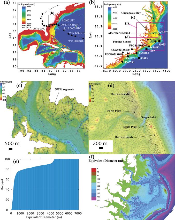
1704                            F. Ye et al.: A cross-scale study for compound flooding processes during Hurricane Florence

                                                                        this event. The trade-off between 2D and 3D setups was care-
                                                                        fully weighed with the goal of operationalization in mind be-
                                                                        fore the 3D setup was chosen. In short, the advantage of 2D is
                                                                        the speed (about 80 times faster than its 3D baroclinic coun-
                                                                        terpart) and the simplicity of the setup; the disadvantage is
                                                                        that it misses baroclinic effects and 3D processes whose im-
                                                                        portance can vary in space and time. For example, the baro-
                                                                        clinic effects during the adjustment phase after Hurricane
                                                                        Irene (2011) are discussed in detail in Ye et al. (2020) us-
                                                                        ing a similar model setup as the one used here. Even though
                                                                        different setups (2D, 3D barotropic, and 3D baroclinic) were
                                                                        tuned to their best possible skills, the 3D baroclinic setup
                                                                        was shown to better capture the total elevation during the
                                                                        post-storm adjustment phase. In addition, during the ongo-
                                                                        ing effort to operationalize the model, we found that includ-
                                                                        ing 3D processes greatly simplified the bottom friction pa-
                                                                        rameterization at some coastal locations (e.g., NOAA Sta-
                                                                        tion 8447930 at Woods Hole, MA; Huang et al., 2021b). A
                                                                        3D model can also produce relevant 3D variables (e.g., 3D
                                                                        velocity and tracer concentration) that are important for safe
                                                                        navigation and ecosystem health. The 3D model presented
                                                                        in this paper is efficient enough for operational forecasts
                                                                        (see Sect. 3.1), which are being set up at NOAA (National
                                                                        Oceanic and Atmospheric Administration).
                                                                           The rest of the paper is structured as follows. Section 2
Figure 1. Weather map showing the low-pressure system and               will review the study site and available observations collected
amount of rainfall Florence brought to the North Carolina and
                                                                        during the event in the watershed, estuaries, and coastal
South Carolina coast around landfall. Credit: NOAA Central Li-
brary US Daily Weather Maps Project (https://www.wpc.ncep.noaa.
                                                                        ocean. Section 3 describes the numerical model used and
gov/dailywxmap/, last access: April 2021); partial views of the orig-   its setup. Section 4 presents model validation and impor-
inal online maps.                                                       tant sensitivity test results; the validation is done in a cross-
                                                                        scale fashion from small-scale watershed areas to large-scale
                                                                        coastal ocean. Section 5 discusses the compound effects as
                                                                        revealed by the 3D model in all regimes. Section 6 summa-
   In this paper, we will study the response to the storm in the        rizes the major findings and planned follow-up work.
watershed rivers and estuaries and examine the processes and
sources that led to the compound flooding there. We will also
examine the coastal responses to the event and the close con-           2   Study site and observation
nection between watershed and coastal ocean. The existing
modeling efforts on compound flooding (Chen et al., 2010;               The focus (high-resolution) area of this study is the NC and
Cho et al., 2012; Dresback et al., 2013; Chen and Liu, 2014;            SC coast and coastal watersheds that saw most of the impact
Ikeuchi et al., 2017; Kumbier et al., 2018; Pasquier et al.,            from Florence (Fig. 3b and f). Similar to what we did for
2019; Wing et al., 2019; Muñoz et al., 2020) often focus on             other hurricane events, the spatial domain’s landward bound-
a subset of the processes (storm surges, tides, waves, fluvial          ary is set at 10 m above the NAVD88 datum, which is deemed
flooding, pluvial flooding, and potential baroclinic effects),          sufficient to capture most backwater effects (Zhang et al.,
leaving gaps in accurately representing the complex inter-              2020). A rich set of observations for physical and biolog-
actions among them (Santiago-Collazo et al., 2019). What                ical variables are available from satellites, autonomous in-
distinguishes this study from traditional compound flooding             struments (e.g., gliders and Argo floats), in situ stations op-
simulations is a holistic approach that solves interrelated pro-        erated by NOAA, and USGS’s field estimates collected dur-
cesses in different regimes and on multiple temporal and spa-           ing after-event surveys (e.g., high water marks or HWMs;
tial scales with the same hydrodynamic core (i.e., the same             Fig. 2b and c). Analysis and quality control of these datasets
set of governing equations) in a single modeling framework.             have been done by the data distributors, together with uncer-
An overview of the processes studied in this paper is shown             tainty assessments. Some of the datasets will be presented
in Fig. 2. The primary tool used in this study is a proven              in the context of model validation sections below to allow
cross-scale 3D baroclinic model designed for effective and              for a comprehensive and objective assessment of the model
holistic simulations of intertwined processes as found during           errors and uncertainties. An assessment of compound flood

Nat. Hazards Earth Syst. Sci., 21, 1703–1719, 2021                                      https://doi.org/10.5194/nhess-21-1703-2021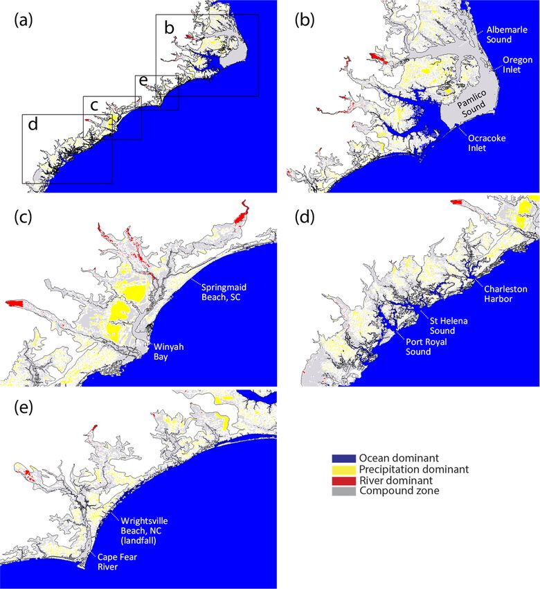
F. Ye et al.: A cross-scale study for compound flooding processes during Hurricane Florence                                        1705

Figure 2. Overview of the processes studied in the paper, from (a) coastal zone to (b) watershed and down to very small local scales in
the watershed in (c) and (d). The base maps in (c) and (d) are provided by Esri (sources: Esri, DigitalGlobe, GeoEye, i-cubed, USDA FSA,
USGS, AEX, Getmapping, Aerogrid, IGN, IGP, swisstopo, and the GIS user community).

models such as ours inevitably involves observations col-             a balance of accuracy, efficiency, robustness, and flexibil-
lected at disparate spatial and temporal scales of several or-        ity include hybrid finite-element and finite-volume methods
ders of magnitude contrasts, as illustrated in Fig. 2. To the         and a highly flexible 3D gridding system (“polymorphism”)
best of our knowledge, this type of model assessment has              that combines a hybrid triangular-quadrangular unstructured
rarely been attempted before even in a 2D setting due to              grid in the horizontal dimension; and localized sigma co-
the formidable challenges to numerical models (Santiago-              ordinates with shaved cells (dubbed as LSC2 ; Zhang et al.,
Collazo et al., 2019) but is badly needed in order to gain a          2015) in the vertical dimension. The polymorphism allows a
holistic understanding of the complex processes at play (Ye           single SCHISM grid to seamlessly morph between full 3D,
et al., 2020; Zhang et al., 2020; Huang et al., 2021a).               2DH (2D depth-averaged), 2DV (2D laterally averaged), and
                                                                      quasi-1D configurations. The employment of shaved cells
                                                                      near the bottom in particular faithfully preserves the original
3     Model description                                               bathymetry without any smoothing required. The detrimen-
                                                                      tal effects of bathymetry smoothing on important physical
3.1    Model setups                                                   and biological processes (e.g., residual transport, lateral cir-
                                                                      culation, nutrient cycling, etc.) have been documented in Ye
To capture the storm surge effects we use a large study do-           et al. (2018) and Cai et al. (2020).
main that encompasses the North Atlantic west of 60◦ W                   Similar to a recent compound flooding study using
(Fig. 3a). An added benefit of using such a large domain              SCHISM for Hurricane Harvey (Huang et al., 2021a), the
in conjunction of a 3D baroclinic model is that the interac-          current model domain covers the entire US east coast and
tion between large- and small-scale processes can be organi-          the entire Gulf of Mexico, with all major bays, estuaries,
cally examined in a single model. For example, the disruption         and coastal watersheds resolved (Fig. 3). The horizontal
and oscillation of the Gulf Stream by storms can directly af-         grid, generated using the software SMS (aquaveo.com), has
fect the coastal inundation (i.e., the fair-weather flooding re-      2.2 million nodes and 4.4 million elements (Fig. 3). About
ported by Ezer, 2018); our results suggest that the converse          50 % and 40 % of the elements have a resolution finer than
is also true, as watershed processes can also affect the Gulf         300 and 220 m, respectively (Fig. 3e). The grid bathymetry
Stream and other coastal processes (Ye et al., 2020). There-          is interpolated from a combination of digital elevation model
fore, a seamless creek-to-ocean model is advantageous for             (DEM) sources from coarse (ETOPO1, 90 m Coastal Relief
compound flood studies.                                               Model1 ) to fine resolution (1/9 arcsec CUDEM2 and 1–3 m
   As we shall see, this model solves the physical pro-               CoNED3 ), and the vertical datum used is NAVD88, with ap-
cesses from the watershed to the ocean with the same                  propriate conversion between datums done by the VDatum
set of governing equations, qualifying for the definition of          tool (vdatum.noaa.gov). Note that NAVD88 is a more conve-
Santiago-Collazo et al. (2019) of a fully coupled compound
surge and flood model. SCHISM (schism.wiki) uses effi-                   1 https://ngdc.noaa.gov/mgg/coastal/crm.html, last access: Jan-
cient semi-implicit solvers to solve the hydrostatic form of          uary 2021.
the Reynolds-averaged Navier–Stokes equations and trans-                 2 https://www.ncei.noaa.gov/metadata/geoportal/rest/metadata/
port equation (Zhang et al., 2016) which govern all flow              item/gov.noaa.ngdc.mgg.dem:999919/html, last access: Jan-
movements inside the 3D model domain, including over-                 uary 2021.
land flow in the watersheds, as well as estuarine and ocean              3 https://www.usgs.gov/core-science-systems/eros/coned,     last
circulations. Major characteristics of the model that ensure          access: January 2021.

https://doi.org/10.5194/nhess-21-1703-2021                                    Nat. Hazards Earth Syst. Sci., 21, 1703–1719, 2021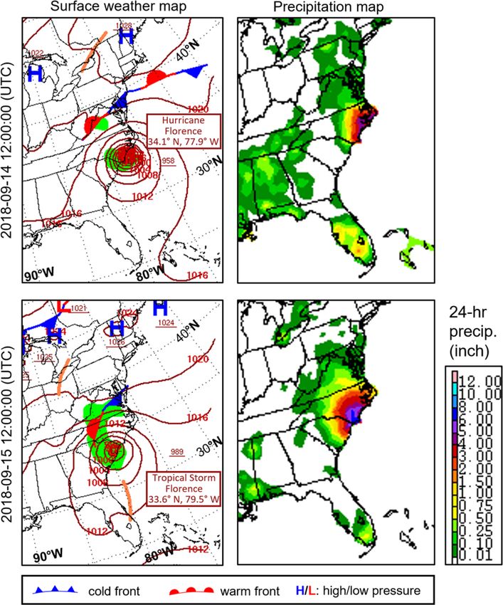
1706                            F. Ye et al.: A cross-scale study for compound flooding processes during Hurricane Florence

Figure 3. Model domain and horizontal grid. (a) Domain extent and hurricane track. (b) Station locations along the North Carolina and
South Carolina coast. The six NOAA gauges are Charleston (8665530), Springmaid Pier (8661070), Wrightsville Beach (8658163), Beaufort
(8656483), Hatteras (8654467), and Oregon Inlet (8652587). The three squares are National Data Buoy Center (NDBC) buoys (41013, 41159,
and 41025). The spatial extents of (c), (d), and (f) are also marked in (b). (c) Zoom-in of grid in a watershed area (the arcs are from National
Water Model (NWM) river network). (d) Zoom-in of grid near barrier islands and inlet (the dark line is the 0 m isobath, NAVD88). (e)
Cumulative histogram of grid resolution (measured in equivalent diameters). (f) Grid resolution in North Carolina’s coastal watershed area.

Nat. Hazards Earth Syst. Sci., 21, 1703–1719, 2021                                         https://doi.org/10.5194/nhess-21-1703-2021
F. Ye et al.: A cross-scale study for compound flooding processes during Hurricane Florence                                                1707

Figure 4. Vertical grid. (a) Transect from the watershed to the ocean used to illustrate the vertical grid; (b) vertical grid along the transect;
(c) zoom-in from (b) illustrating the transitions from 3D (Pamlico Sound) to 2DH (barrier islands) and back to 3D (coastal ocean). The base
map in (a) is provided by Esri (sources: Esri, DeLorme, HERE, USGS, Intermap, iPC, NRCAN, Esri Japan, METI, Esri China (Hong Kong),
Esri (Thailand), MapmyIndia, Tomtom).

nient datum to use in the model as most of the recent ob-                  Table 1. Baseline and sensitivity runs used in this paper.
servational data refer to this datum, and therefore we use
this datum in the model setup and allow the model to au-                     Scenario            Description
tomatically set up the sub-tidal surface slope from coastal                  Baseline            With forcing from tides, atmosphere, rivers
ocean into watershed (due to the friction effects). Altogether                                   (from NWM), and precipitation, initialized
close to 400 DEM tiles are used to cover such a large re-                                        with HYCOM GOFS 3.1
gion. The horizontal grid resolution ranges from 6–7 km in
the open ocean to ∼ 400 m near the shoreline, with bar-                      Baseline_Wave       Baseline with added wave effects
rier islands and narrow inlets resolved; river channels and                  Ocean               Baseline forced by ocean and atmosphere
creeks have about 300 m along-channel resolution and vari-                                       (i.e., tides and storm surge) only
able cross-channel resolutions to ensure adequate represen-
                                                                             River               Baseline forced by rivers (i.e., freshwater
tation of the channelized flow. Shipping channels are repre-                                     inputs from NWM) only
sented by quadrangles and have 20 m or finer cross-channel
resolution in NC. The finest grid resolution used is ∼ 1 m                   Rain                Baseline forced by precipitation (directly
which represents many levees in other parts of the coast;                                        on top of the domain) only
note that as an implicit model SCHISM is not constraint by
the Courant–Friedrichs–Lewy (CFL) condition and thus can
handle high resolution efficiently. Moreover, to better cap-               thus effectively rendering the model 2DH there, which is suf-
ture the geometry and bathymetry of flood pathways in the                  ficient for processes like overland flow and inundation.
watershed region, specifically the region between the 10 m                    Table 1 shows the setups for Baseline and important sensi-
contour (set as the land boundary) and the 0 m contour of                  tivity simulations used in this paper. For the Baseline, im-
the DEM (based on NAVD88), about 300 000 National Water                    posed at the ocean boundary (60◦ W) are tidal elevation
Model (NWM) segments (i.e., thalwegs; Fig. 3c) are repro-                  and barotropic velocity of eight tidal constituents (S2, M2,
duced in SCHISM’s horizontal grid. Note that only the ge-                  N2, K2, K1, P1, O1, and Q1) extracted from the FES2014
ometry of the NWM segments is retained, while NWM out-                     database4 . The baroclinic components for the elevation and
puts are only used as the land boundary condition, and NWM                 velocity are derived from the daily outputs of the HYbrid
does not solve any hydrodynamics inside the model domain.                  Coordinate Ocean Model (HYCOM; hycom.org). The initial
Customary of all SCHISM applications, no manipulation or                   condition for the water elevation is set to be 0 in all areas
smoothing of bathymetry was done in the computational grid                 with positive grid depths (“wet” with 0 initial water level,
after interpolation of the depths from DEMs (including steep               e.g., rivers and bays) and to be equal to the bottom eleva-
slopes in the Caribbean and all shipping channels). From our               tion in areas with negative grid depths (“dry” with 0 initial
experience, CUDEM may underestimate the depth of coastal                   water depth, e.g., high ground in the watershed). The initial
streams (e.g., those in the South Carolina watersheds), which              condition for the horizonal velocity is zero in the watershed
is a potential error source of our model. In the vertical dimen-           and is interpolated from HYCOM elsewhere. Commensurate
sion we use 1–43 grid layers, with 43 layers being applied in              with the non-zero velocity (fully dynamic state) are salin-
the deep ocean and 1 layer in most of the watershed (Fig. 4),
                                                                              4 https://datastore.cls.fr/catalogues/fes2014-tide-model/, last ac-
                                                                           cess: January 2021.

https://doi.org/10.5194/nhess-21-1703-2021                                          Nat. Hazards Earth Syst. Sci., 21, 1703–1719, 2021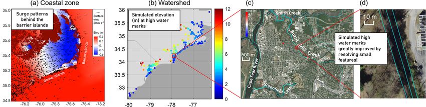
1708                            F. Ye et al.: A cross-scale study for compound flooding processes during Hurricane Florence

ity and temperature values interpolated from HYCOM; how-               quasi-2D, making it efficient enough for operational fore-
ever, in the nearshore areas where HYCOM results are less              casts. For the Baseline run, the real time to simulation time
accurate, the initial conditions for salinity and temperature          ratio is 80 with 1440 cores on TACC’s (Texas Advanced
are interpolated from the sparse observation at several USGS           Computing Center) Stampede2 cluster and 30 with 480 cores
gauges in order to speed up the dynamic adjustment process.            on W&M’s SciClone cluster. Intel Skylake cores with a nom-
The surface meteorological forcing applied in the model is             inal clock speed of 2.1 GHz were used on both clusters. This
a combination of two products: (1) a high-resolution ERA               means a 3 d (typical operational forecast duration) simula-
re-analysis product from the European Centre for Medium-               tion will take about 0.9 h using 1440 cores or 2.4 h using
range Weather Forecasts (ECMWF) with a ∼ 9 km horizontal               480 cores.
resolution (see Acknowledgements) and (2) a 3 h time inter-
val with NOAA’s High-Resolution Rapid Refresh (HRRR5 ),                3.2   Coupling with NWM
which is a cloud-resolving and convection-allowing atmo-
spheric model with a 3 km horizontal resolution and a 1 h              River discharges are introduced into our model at its land
time interval. The friction of the Baseline model was tuned in         boundary. About 6752 intersection points are identified be-
the wet area (river, estuary, ocean; lower than 1 m, NAVD88)           tween the NWM river segments and SCHISM’s land bound-
and on higher grounds (higher than 3 m, NAVD88) sepa-                  ary where the freshwater is injected as volume sources
rately. In the wet area, drag coefficients within a range of           (Fig. 5). Inside the model domain, streamflow, overland flow,
0.001–0.01 (non-dimensional) were tested. The commonly                 and precipitation are directly handled by the hydrodynamic
accepted default value of 0.0025 gave good error statistics            core of SCHISM. This fully coupled configuration is rare
near the landfall site, and values within a range of 0.001–            in the existing compound flooding simulations (Santiago-
0.005 gave very similar results. In the watershed, drag co-            Collazo et al., 2019). To ensure the accuracy and robust-
efficients within a range of 0.01–0.5 were tested. The opti-           ness of SCHISM in simulating hydrological and hydraulic
mal value was chosen based on the high water mark (HWM)                processes including the overland flow, we already examined
comparisons (Sect. 4.3) at 276 locations recorded by USGS.             the model’s performance in both lab-scale and field-scale
A small friction value within this range tended to underpre-           tests in a previous study (Sects. 2.2 and 2.3 of Zhang et al.,
dict the elevation at HWMs, and a large value led to over-             2020) and applied the model in the Delaware Bay watershed
prediction. Values within a range of 0.02–0.05 gave good er-           including the Delaware River (extended to 40 m above the
ror statistics. We chose 0.025 because it gave slightly bet-           NAVD88 datum) with a hydraulic jump (Fig. 14 in Zhang
ter results in the Cape Fear River watershed near the land-            et al., 2020). The NWM segments explicitly reproduced in
fall site. To sum up, drag coefficient is set at a constant            our grid (Fig. 3c) during the mesh generation stage help
value of 0.0025 at all “wet” locations and then linearly in-           capture the bathymetry of main flood pathways (thalwegs).
creased to 0.025 as the ground elevation increases from 1              However, flow is not restricted to these 1D segments; in fact,
to 3 m (NAVD88), and finally a constant value of 0.025 is              precipitation may generate overland flow on any 2D horizon-
used for higher grounds where the bed texture is generally             tal grid elements in the watershed. Note that the river flows
rougher than the riverbed. Note that this is the parameteriza-         injected at the land boundary have indirectly incorporated
tion based on the region influenced by Hurricane Florence.             the precipitation that occurred outside (but not inside) the
Spatially varying parameterization of bottom friction for dif-         model domain, and therefore, the addition of direct precipita-
ferent systems is an ongoing effort as we study more recent            tion onto the model domain is appropriate and is an integral
hurricanes and operationalize the model along the east coast           component of the compound flood processes. To accurately
and the Gulf Coast. However, as presented in Ye et al. (2020),         simulate the initial movement of the very thin layer of rain-
Zhang et al. (2020), and Huang et al. (2021a), the choices             water on the dry land, which is dominated by friction, a very
described above seem to work fine in general for other sys-            small threshold of 10−6 m is used to differentiate between
tems as well. The method used to impose the river flow in the          wet and dry states (Zhang et al., 2020). Since we have no in-
model is described in the next subsection.                             formation on the scalar concentrations for river inflows and
   Choices of the Baseline model parameters are similar to             rainfall, we applied 0 PSU (practical salinity unit) for salin-
those used for Irene (Ye et al., 2020). The time step is 150 s         ity and ambient water temperature (i.e., the temperature at
(sensitivity tests using 100–150 s gave very similar results).         the local receiving cell calculated without accounting for the
The level-2.5 equation turbulence closure scheme chosen is             rivers or raindrops) for the injected river water and also for
from the generic length scale model k-kl (Umlauf and Bur-              the rainfall. Obviously, the latter represents a source of un-
chard, 2003). The simulation starts from 24 August 2018 at             certainty for the modeled temperature results. As explained
00:00 UTC and lasts for 36 d to cover the hurricane and en-            in Huang et al. (2021a), heat exchange between air and water
suing restoration period. Although the model covers a large            would misbehave on such a thin layer of water in the water-
domain, most of the elements (those in the watersheds) are             shed, so a threshold of 0.1 mm is set for local water depth,
                                                                       below which the heat exchange is turned off. As a model
   5 https://rapidrefresh.noaa.gov/hrrr/, last access: January 2021.   limitation, infiltration is neglected in this work. In the case

Nat. Hazards Earth Syst. Sci., 21, 1703–1719, 2021                                    https://doi.org/10.5194/nhess-21-1703-2021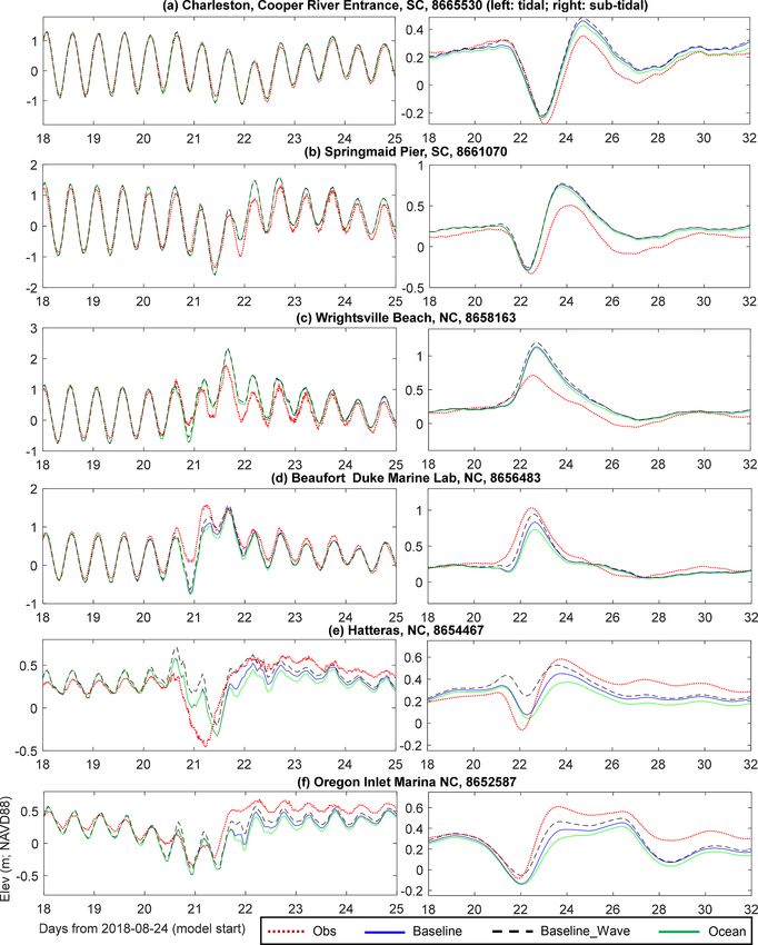
F. Ye et al.: A cross-scale study for compound flooding processes during Hurricane Florence                                            1709

Figure 5. Distribution of river discharge (time-averaged during the simulation period) in North Carolina and South Carolina from the National
Water Model (NWM).

of Hurricane-Florence-induced flooding, we expect the ef-                tion indicates the peak streamflow occurs about 7 d after the
fect of infiltration to be minor. According to NOAA’s weather            landfall, which is the time it takes for the rainfall-induced
map6 , there was continuous rainfall along the US east coast             flood to reach the coastal rivers. Note that there is typically
from 11 September 2018 to the date of Florence’s landfall                a time lag of 1–2 d between the peak flow in NWM and the
(14 September 2018), so the infiltration capacity of the soil            gauged flow (Fig. 6). The forcing errors in the magnitude
was already reduced. Moreover, “wet” storms like Hurricane               and timing of NWM’s peak flow should explain part of the
Florence (2018) and Hurricane Harvey (2017) tend to dump                 model errors, especially in the watershed. For example, we
a large amount of rain fall at a location for days because               found that replacing the NWM streamflow with the gauged
of the slow movement of the storm, so most of the rainfall               flow at USGS Station 02109500 (Waccamaw River at Free-
should be on saturated soil. As another model limitation, the            land, NC) improves the model skill locally. However, this is
drainage in urban settings is not included in our model. This            not cost-effective for our goal of operationalizing this com-
may have led to some occasional big errors in the predicted              pound flood model along the US east coast and Gulf Coast.
elevation on high water marks, for example the one large er-             The developers of NWM (Gochis et al., 2018) showed that
ror in the urban area in Fig. 13d. We do have a plan of explic-          NWM’s model skill was improved by each version update,
itly accounting for infiltration and drainage as volume sinks            with 44 % of the gauges having a bias < 20 % in the lat-
based on NWM (or other hydrologic models). However, con-                 est version (NWM v2.0). We will adopt the newest and best
sidering the additional uncertainty this would bring, for now            NWM version as soon as it is available in our ongoing study
we choose to continue improving more important aspects of                and operational forecast, and we are open to using any other
the model for operational use; the focus is on the quality of            hydrologic sources to drive our model.
model grid, which is very likely responsible for most of the
existing large errors.
   The assessment of NWM-calculated flow against observed
                                                                         4   Model validation and sensitivity
flow at the two largest rivers in the region is shown in Fig. 6.
Similar to our findings for other storm events, the flow pro-
                                                                         In this section we will assess the model results for elevation,
duced by this particular version of NWM (v2.0) is gener-
                                                                         inundation, and flow in the watershed and estuary. The spa-
ally consistent with USGS observations but tends to show
                                                                         tial scales covered by the validation vary from O(10 km) to
narrower and higher peaks, with roughly the same total vol-
                                                                         O(1 m). The model validation for non-storm period will not
ume of water throughout the event (Fig. 6). The observa-
                                                                         be discussed here; in short, the averaged amplitude error for
  6 https://www.wpc.ncep.noaa.gov/dailywxmap/,        last   access:     the major constituent (M2 on east coast and K1 in north-
April 2021.                                                              ern Gulf of Mexico) for the non-storm period is 3–4 cm (see

https://doi.org/10.5194/nhess-21-1703-2021                                      Nat. Hazards Earth Syst. Sci., 21, 1703–1719, 2021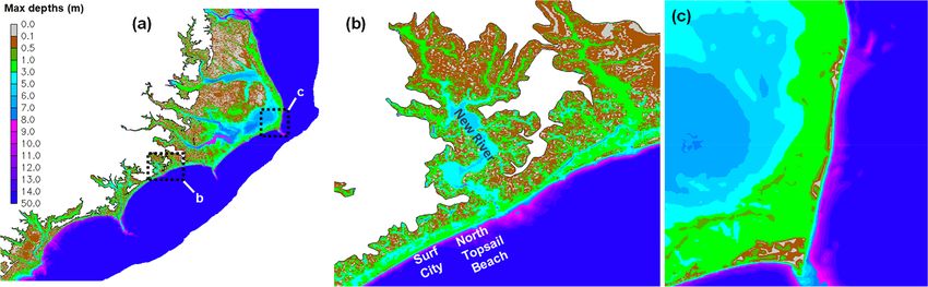
1710                          F. Ye et al.: A cross-scale study for compound flooding processes during Hurricane Florence

Figure 6. Discharges at the two largest freshwater sources in the impact region (locations marked in Fig. 5). At each location, the NWM
streamflow is taken at the intersection of the NWM segment and SCHISM’s land boundary; the observation is based on the closest USGS
station.

Huang et al., 2021a). We will start by looking at the wave            and 24 frequency bins to cover a frequency range of 0.04 to
effects nearshore.                                                    1 Hz. The coupling time step between the two models (i.e.,
                                                                      the interval at which the information of surface elevation, ve-
4.1 Wave effects                                                      locity, and wave radiation stress was exchanged) was 600 s.
                                                                          Our results indicate that the barrier islands near Surf City,
Multiple breaches and over-toppings were reported7 across             North Top Sail Beach, and New River inlet were indeed over-
several NC barrier islands during the event, including Surf           topped with 1–2 m of water (Fig. 7b; the locations of the is-
City, North Top Sail Beach, and New River inlet. Some of              lands can be seen in Fig. 8b). On the other hand, a large por-
these breaches may be related to significant wave activi-             tion of the island north of Cape Hatteras (Outer Banks) was
ties; for example, the maximum wave height at buoy 41025,             spared (Fig. 7c) likely due to its north–south shoreline ori-
∼ 30 km offshore from Cape Hatteras, reached ∼ 10 m. Inter-           entation, even with the 10 m wave approximately 30 km off-
estingly, the maximum wave heights become relatively mod-             shore from there. More quantitative validation for the breach-
est nearer to the landfall: 4–6 m at buoys 41159 and 41013            ing processes is beyond the scope here because (1) we do
(see Fig. 3b for their locations). Therefore, to investigate this     not have accurate and up-to-date bathymetry just before the
possibility, we have also conducted a simulation with the             event and (2) more importantly, a sediment transport study is
wave model in SCHISM activated (Baseline_Wave in Ta-                  required to simulate the bathymetric changes.
ble 1). The details of the wave model (Wind Wave Model)                   The wave effects on the surface elevation are further quan-
have been described in Roland et al. (2012), and the cou-             tified in Fig. 8, which suggests that the effects are most pro-
pled model has been applied to other systems (Guérin et al.,          nounced (with 30 cm or larger differences) inside the estuar-
2018; Khan et al., 2020). The wave model was initialized and          ies and Albemarle–Pamlico Sound (APS) due to large wave
forced at the ocean boundary by a global Wave Watch III sim-          breaking nearby. In the intermediate and deep water, how-
ulation8 and used a spectral resolution of 36 directional bins        ever, the wave effects are on the order of a few centimeters
   7 https://www.wusa9.com/article/weather/                           and negligible (Fig. 8a). The Baseline results (without wave
before-and-after-hurricane-florence-changes-north-carolina-coastline/ effects) also showed over-topping of the barrier islands sim-
65-595918389, last access: 29 May 2021.                               ilar to the Baseline_Wave (not shown).
   8 ftp://ftp.ifremer.fr/ifremer/ww3/HINDCAST, last access: Jan-
uary 2021.

Nat. Hazards Earth Syst. Sci., 21, 1703–1719, 2021                                    https://doi.org/10.5194/nhess-21-1703-2021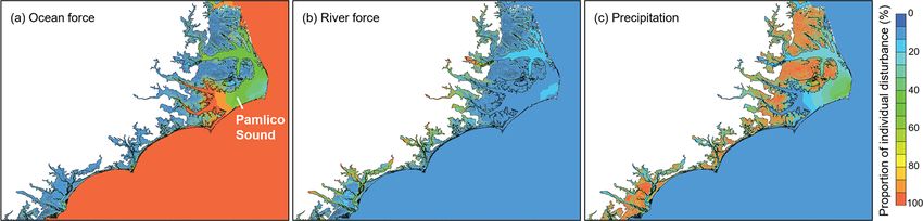
F. Ye et al.: A cross-scale study for compound flooding processes during Hurricane Florence                                         1711

Figure 7. The maximum water depths from Baseline_Wave. The spatial extents of the local regions of (b) and (c) are marked in (a).

Figure 8. Differences of the maximum elevations between Baseline_Wave and Baseline. Panel (b) is a zoom-in on (a). The thin black lines
are the 0 m isobath.

   In summary, the wave effects are significant nearshore              of ∼ 0.2–0.5 m and surges of ∼ 0.5–1 m at Wrightsville and
and have contributed to the observed breaching and over-               Beaufort (Fig. 9). The different responses at these gauges
toppings of barrier islands. However, because the current              are due to the wind curl of Florence that led to different
study does not focus on the breaching processes and be-                dominant wind directions between southern and northern sta-
cause of the significant computational overhead introduced             tions and are also due to specific geographic settings of each
by adding the wave model (> 50 %), we will proceed in the              gauge. Most intriguing are the prominent set-downs observed
following by using the run without waves as the Baseline.              at Hatteras and Oregon Inlet, which are explained by a com-
                                                                       bination of wind direction and blocking effects of barrier is-
4.2   Bays and estuaries                                               lands. Figure 10 demonstrates that around the time of land-
                                                                       fall of the hurricane, the predominantly westward wind felt
We assess the calculated water levels at six NOAA tide                 in the Pamlico Sound has pushed water away from the bar-
gauges near the impact area (see locations in Fig. 3b). Three          rier islands. Meanwhile, the surge that propagated from the
gauges are facing the open ocean (Charleston, Springmaid,              ocean side is effectively blocked by the barrier island chain,
and Wrightsville), and the other three gauges are either shel-         thus creating a ∼ 70 cm elevation difference between the wa-
tered inside a bay (Beaufort) or behind barrier islands (Hat-          ters immediately outside and inside the islands (Fig. 10).
teras and Oregon Inlet). The responses to the hurricane are            The mechanism causing the water level set-downs at the two
different at those gauges, as seen from the total elevation            South Carolina stations (Charleston and Springmaid) is simi-
(Fig. 9a) and the sub-tidal signals (Fig. 9b). The latter applies      lar to that causing the set-downs behind the barrier islands in
a low-pass Butterworth filter (Butterworth, 1930) only pre-            North Carolina. The two South Carolina stations are located
serving longer-period (longer than 2 d) components. The ob-            to the south of the landfall site, and the wind direction is from
servation shows sea set-downs of ∼ 0.3–0.5 m at Charleston,            the land to the ocean, pushing water away from shore. The
Springmaid, Hatteras, and Oregon Inlet followed by surges

https://doi.org/10.5194/nhess-21-1703-2021                                    Nat. Hazards Earth Syst. Sci., 21, 1703–1719, 2021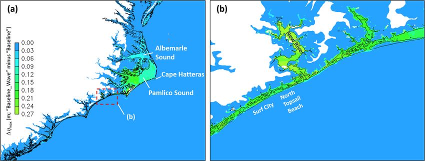
1712                           F. Ye et al.: A cross-scale study for compound flooding processes during Hurricane Florence

Figure 9. Comparison of elevation at six NOAA gauges: (left) total elevation; (right) subtidal elevation. Also included are results from two
sensitivity runs (Baseline_Wave and Ocean; see descriptions in Table 1). Note the plots have different y-axis ranges.

model captured the different regional responses; overall, the           a maximum overprediction of 0.64 m for the peak surge at
averaged MAE (mean absolute error) for elevation is 11 cm.              Springmaid Pier, SC. The overpredicted peak surge can lead
The averaged MAE for the subtidal comparison is 8.6 cm,                 to overpredictions in elevation on coastal high water marks
and the averaged correlation coefficient is 0.92. The peak er-          (HWMs). In addition, there is a maximum underprediction
rors at different stations occur around the storm surge, with           of 0.66 m for the set-down at Hatteras, NC, mainly due to the

Nat. Hazards Earth Syst. Sci., 21, 1703–1719, 2021                                       https://doi.org/10.5194/nhess-21-1703-2021
F. Ye et al.: A cross-scale study for compound flooding processes during Hurricane Florence 1713
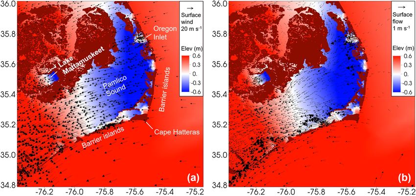
Figure 10. Snapshots of water surface elevation at the time of Florence’s landfall (14 September 2018) near the barrier islands around
Pamlico Sound, overlaid by (a) wind speed at water surface and (b) surface flow. Note that the general pattern of wind-induced set-up and
set-down is also present on a smaller scale (Lake Mattamuskeet).
Figure 11. Comparison of water surface elevation on HWMs. (a) Field estimates from USGS; (b) model prediction; (c) model minus
observation; (d) regression between model prediction and observation; (e) histogram showing the error distribution.
mismatch in the set-down timing. The uncertainties in wind are derived from small seeds or floating debris carried by
forcing may be the main cause of the error, which is predomi- floodwaters that adhere to smooth surfaces or lodge in tree
nantly from subtidal signals. The grid quality near the barrier bark to form a distinct line and also by stain lines on build-
islands may also contribute to the error. Adding wave effects ings, fences, and other structures. Therefore, HWMs are time
slightly increases the surge and rebounding waves at the last sensitive and usually have vertical uncertainties of ±0.3 ft
three gauges, resulting in slightly better model skills there. or equivalently ±0.09 m (Koenig, et al., 2016; Austin, et al.,
2018).
4.3 Watershed The simulated elevation on 276 HWMs in the NC and SC
watersheds are compared with field estimates (Fig. 11). The
High water marks (HWMs) were collected by USGS experts model is able to capture the transition from estuarine to river-
more than 2 weeks after Hurricane Florence’s landfall. They ine regimes; note that the averaged bottom elevation for all
https://doi.org/10.5194/nhess-21-1703-2021 Nat. Hazards Earth Syst. Sci., 21, 1703–1719, 20211714 F. Ye et al.: A cross-scale study for compound flooding processes during Hurricane Florence
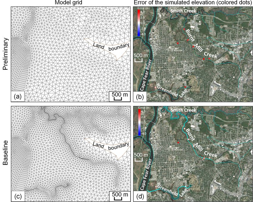
ing of water locally and thus large overprediction of HWMs
there. The channel of the creek is about 6–10 m wide, and
once resolved using two rows of quadrangles as was done in
the Baseline (Fig. 13c), the model skill was greatly improved
(Fig. 13d). The only remaining large error point in the Base-
line occurs in an urban area away from the river (Fig. 13d)
likely due to the building or drainage effects that have not
been incorporated in the model. The defects in grid quality
can lead to large errors that are not likely to be rectified by
tuning other parameters. To fix the remaining few large er-
rors away from the landfall site, grid quality should be exam-
ined first. The continuous improvement on this model grid
is part of an ongoing effort of operationalizing the model
Figure 12. Model–data comparison near the landfall location: (a) along the US east coast and Gulf Coast, and we will report
streamflow; (b) gauge height. The sensitivity run (without freshwa- this in future studies. Resolving small-scale flow routing fea-
ter inputs from NWM or precipitation) is also shown, in which the tures on a national scale requires automated tools such as
channels are dry even during the hurricane, indicating they are be- Pysheds9 that can detect and delineate the channels automat-
yond the storm surge influence. The station location is marked in ically. Initial tests showed very promising results from this
Fig. 3b.
package. We remark that it is feasible to resolve these fea-
tures efficiently without significantly increasing the grid size
due to SCHISM’s flexibility and robustness in handling poor-
observation points is 3.8 m (NAVD88), and about 70 % of the quality meshes. Afterwards, the inclusion of urban drainage
points are located above 2 m (NAVD88), beyond the reach of should reduce the occasional large errors there. Other fac-
storm surges. Overall, the averaged MAE for all HWMs is tors such as uncertainties in DEM, precipitation, and the river
0.73 m, with a correlation coefficient of 0.92 and a positive flow through land boundary also play minor roles.
mean bias of 0.09 m. There is a slight positive bias on near-
shore HWMs (Fig. 11) corresponding to the overprediction
of peak elevation at coastal stations (Fig. 9a–c). These skill 5 Compound effects
scores are similar to what we obtained for Hurricane Harvey
A carefully validated 3D model such as the one presented
(Huang et al., 2021a).
here can effectively separate out compounding factors from
Figure 12 shows the comparison for both elevation (gauge
different sources: coastal surge, river flooding, and precipi-
height) and discharge in a large river in the study region.
tation. In this section we apply this approach to examine the
The gauge is in the interior of our grid, near “Freshwater
contributing factors to the total flooding during Florence. The
Source 2” in Fig. 6. Because the observation’s vertical da-
design of the numerical experiments is such that we selec-
tum is NAVD29 and the model’s datum is NAVD88, we
tively turn on and off forcing from ocean, river, and precip-
have adjusted the mean model elevations to match the ob-
itation to examine their individual effects in isolation (Ta-
served mean in the elevation comparison (Fig. 12b); in other
ble 1). As an overview, the conditions of maximum inunda-
words, only the elevation variability is compared. Our model
tion extent from all scenarios are listed in Table 2. To facili-
overpredicted the flow and underpredicted the flood-induced
tate the comparison of inundated area, a practical value (1 ft,
surges. Using a more accurate fresh water source at the land
or equivalently 0.305 m) on the same order of the mean inun-
boundary, improving the channel representation in the model
dation depth is used as a threshold. For the two indices (per-
grid, and locally adjusting the bottom friction should help
cent inundated area and maximum inundation depth) shown
improve the skill.
in Table 2, the Baseline values are significantly larger than
Our tests show that the simulated elevation on the high
those from a single sensitivity test. This confirms the exis-
water marks (HWMs) in the watershed is sensitive to grid
tence of compound regions in the two states (North Carolina
resolution, precipitation, river inputs through the land bound-
and South Carolina) during the event. More details of each
ary, and bottom friction. Grid resolution and quality are the
forcing’s effect and the compound effects are discussed be-
most important factors. Misrepresenting flood pathways can
low.
easily lead to errors of a few meters near some very local-
Turning off both rivers and precipitation (i.e., ocean only)
ized features such as ditches and highways. Figure 13 illus-
is expected to have a major impact on flooding in the wa-
trates such an example around Burnt Mill Creek in the city of
tershed. This is confirmed in Fig. 12 in the previous section.
Wilmington, NC. Large HWM errors were found in the pre-
Not surprisingly, without rivers and precipitation, watershed
liminary setup because the computational grid did not resolve
the small creeks that served as the main conduit in draining 9 https://github.com/mdbartos/pysheds, last access: Jan-
out the storm water after the flood. This resulted in the stack- uary 2021.
Nat. Hazards Earth Syst. Sci., 21, 1703–1719, 2021 https://doi.org/10.5194/nhess-21-1703-2021F. Ye et al.: A cross-scale study for compound flooding processes during Hurricane Florence 1715
Figure 13. Importance of resolving small-scale features on the order of a few meters in the watershed, illustrated by a comparison between
a preliminary setup (a, b) and the Baseline setup (c, d). To better resolve Burnt Mill Creek, NC, more SMS feature arcs (cyan lines in d) are
used in the Baseline setup than in the preliminary setup (cyan lines in b), significantly reducing the HWM errors. See Fig. 2 for the location
of this locally zoomed-in region. The base maps in (b) and (d) are provided by Esri (sources: Esri, DigitalGlobe, GeoEye, i-cubed, USDA
FSA, USGS, AEX, Getmapping, Aerogrid, IGN, IGP, swisstopo, and the GIS user community).
Figure 14. Simulated water surface elevation on HWMs from the sensitivity run “Ocean”, i.e., without the freshwater inputs from NWM or
precipitation. Note the underpredictions in the watershed and worse model skill compared with Baseline (Fig. 11).
is mostly dry as the storm surge cannot propagate over steep the near-shore HWMs because those locations are predomi-
terrains. As a result, the predicted HWMs are biased too low nately affected by oceanic processes.
(Fig. 14), as the steep topography quickly damped out any Less obvious are the effects of rivers and precipitation on
surges brought in by the ocean. This leads to systematic un- the observed surges in the coastal bays. Figure 9 indicates
derpredictions in the watershed and a 64 % increase in MAE that the effects are negligible at the three coastal stations
compared to the Baseline (Fig. 11). On the other hand, Zhang away from barrier islands (Fig. 9a–c), as the large amount of
et al. (2020) demonstrated that the storm surges can propa- freshwater from the watershed directly drains into the coastal
gate much further into watershed if watershed rivers are in- ocean (which has a much larger volume of water). On the
cluded. There is no apparent deterioration of model skill on other hand, the impounding effects are clearly seen at the two
stations behind the barrier islands (Fig. 9ef; roughly starting
https://doi.org/10.5194/nhess-21-1703-2021 Nat. Hazards Earth Syst. Sci., 21, 1703–1719, 20211716 F. Ye et al.: A cross-scale study for compound flooding processes during Hurricane Florence
Figure 15. Regional map showing the spatially varying importance of each forcing factor: (a) ocean force (Ocean in Table 1); (b) river force
(“River” in Table 1); and (c) precipitation (“Rain” in Table 1). The value is the proportion of a factor’s individual “disturbance” (see definition
in Sect. 5) to the sum of the disturbance from all factors. The colors from blue to red represent the increasing importance of a factor at a
specific location.
Table 2. Overview of the maximum inundation extent in South Car- shed, D represents the local water depth, whereas at initially
olina and North Carolina watersheds (above the NAVD88 datum) “wet” locations, D is simply the surface elevation. D is also
during the simulation period. a smoother metric to measure the compound effects as one
transitions from oceanic into watershed regimes.
Scenario Percentage of Spatially averaged The comparison between the maximum disturbances from
inundated area with maximum inundation the three experiments using only one of the three forcing fac-
water depth > 0.305 m depth (m) tors and the total sum helps elucidate the contributions from
(1 ft)
each. The results are presented in Fig. 15 in terms of pro-
Baseline 46.7 % 0.61 portion of total maximum disturbance as explained by each
Ocean 12.7 % 0.12 forcing factor at a given location (therefore, the sum of all
River 17.4 % 0.31 proportions equals unity). Our results clearly indicate that (1)
Rain 34.4 % 0.36 the ocean (and atmospheric) forcing dominates in the open
ocean and part of southern Pamlico Sound in the APS sys-
tem, (2) river forcing is most dominant in the river network of
from day 22), where the discharged water is trapped for al- watershed, and (3) precipitation effects are dominant in other
most a week. As we showed in Sect. 4.2, the barrier islands parts of the watershed away from the river network. However,
are effective in creating separation and thus a large elevation the presence of the barrier islands significantly complicates
gradient between water immediately outside and inside (see the interaction among different forcings (e.g., the significant
Fig. 10). contribution from precipitation in Pamlico Sound as shown
To assess the contributions from each of the three forcing in Fig. 15c). On the other hand, the inclusion of the wave ef-
factors to the total sum, we follow Huang et al. (2021a) and fects is not expected to alter the findings here because their
use the concept of “disturbance”. We recognize that for com- contribution to the total elevation is relatively minor as com-
pound flooding processes involving both ocean and water- pared to the atmospheric effects (see Fig. 9).
shed, neither the water surface elevation nor the water depth The competition among different forcing factors in differ-
is a satisfactory metric because the nominally large water el- ent regions can be succinctly summarized in a “dominance”
evations on the high ground of the watershed are dominated map as shown in Fig. 16: a factor is deemed dominant if it
by the high bottom elevation there, and the large water depths explains at least 80 % of the total disturbance; if, however,
in the bays and ocean are dominated by the local bathymetry. none of the three factors contribute to 80 % or more at a par-
Therefore, we adopt the concept of disturbance, defined as ticular place, the nonlinear compound effects are expected to
be significant there. The ocean response is overwhelmingly
η, if h ≥ 0, dominated by the oceanic and atmospheric forcing, the re-
D=
η + h, if h < 0, sponse in the watershed rivers by the river flow, and the re-
where η is the water surface elevation and h is the bathymetry sponse in a large portion of highly elevated watersheds by
(positive downward based on the same datum as η; e.g., the precipitation, as seen in Fig. 16. Most of the response in
h > 0 for ocean and h < 0 for high grounds in watershed), the southern Pamlico Sound is of oceanic origin because of
so (η + h) is water depth. Basically, D represents the de- the wider openings to the south (e.g., Ocracoke Inlet). On
parture from “initial condition” (either the initial water sur- the other hand, there are only a few narrow inlets to the east
face or bottom, whichever is higher). Note that D is contin- (e.g., Oregon Inlet), thus effectively blocking off the oceanic
uous across h = 0. On the initially “dry” ground in water- influence there (Fig. 16b; also see Fig. 10). It is the “grey
Nat. Hazards Earth Syst. Sci., 21, 1703–1719, 2021 https://doi.org/10.5194/nhess-21-1703-2021F. Ye et al.: A cross-scale study for compound flooding processes during Hurricane Florence 1717
Figure 16. Dominance map showing the spatial dominance of different flood drivers during Hurricane Florence. Panels (b–e) are zoom-ins
from (a) in different regions.
areas” (Fig. 16) of compound flooding zones that are most for a holistic management approach in the planning of miti-
intriguing. These include most of the APS and coastal rivers gation efforts for the flood hazard during and after hurricane
(Fig. 16b), where the weakened oceanic influence competes events.
with river flow and large rainfall there (Fig. 15). In the estu-
aries with large river discharges and limited openings to the
coastal ocean (Fig. 16c and e), the compound flooding zone 6 Conclusions
is a result of the competition among all three factors. On the
other hand, the estuaries to the south of the landfall site have We have successfully applied a 3D cross-scale model to ex-
smaller river discharges and less precipitation; moreover, amine the compound flooding processes that occurred dur-
they are not protected by barrier islands. As a result, oceanic ing Hurricane Florence 2018. The model is fully coupled in
effects can penetrate very deep into these coastal watersheds the sense that the hydrologic and hydrodynamic processes
(Fig. 16d). Note that the ocean dominance near Wrightsville are solved by the same set of governing equations. Limita-
Beach, NC (NOAA Station 8658163), and Springmaid Pier, tions of the model include the neglection of infiltration and
SC (NOAA Station 8661070), may be exaggerated, consider- urban drainage, which will be implemented soon. The model
ing the overestimated peak elevation there (Fig. 9). The com- was validated with observation data collected in the water-
pound map in Fig. 16 clearly demonstrates the urgent need shed and coastal ocean. The mean absolute errors for major
variables are 11 cm for coastal elevation and 72 cm for high
https://doi.org/10.5194/nhess-21-1703-2021 Nat. Hazards Earth Syst. Sci., 21, 1703–1719, 20211718 F. Ye et al.: A cross-scale study for compound flooding processes during Hurricane Florence
water marks (HWMs). Locally very high resolution was used Financial support. This work is funded by the NOAA Water Ini-
in some watershed areas to resolve small features that were tiative (grant no. NA16NWS4620043). The computational resource
critical for a good model skill for the HWMs. The wave ef- on XSEDE (grant no. TGOCE130032) is funded by the National
fects were found to be significant near barrier islands and Science Foundation (grant no. OCI 1053575).
have contributed to over-toppings and breaches there. The
validated model was then used to reveal significant nonlinear
compound effects in most parts of coastal watersheds and be- Review statement. This paper was edited by Philip Ward and re-
viewed by three anonymous referees.
hind the barrier islands. The barrier islands were shown to be
particularly effective in separating the processes in the water
bodies on the land side and on the ocean side.
The results of the current study, especially the regional
compound zone map, filled in a critical knowledge gap in our References
understanding of compound flooding events. In fact, opera-
tional forecasts based on the current model are being set up Austin, S. H., Watson, K. M., Lotspeich, R. R., Cauller, S. J.,
at NOAA to help coastal resource and emergency managers White, J. S., and Wicklein, S. M.: Characteristics of peak
streamflows and extent of inundation in areas of West Vir-
with disaster planning and mitigation efforts. The model can
ginia and southwestern Virginia affected by flooding, June 2016
also be used to facilitate new scientific discoveries of novel (ver. 1.1, September 2018), US Geological Survey Open-File Re-
coastal processes; for example, preliminary results for the port 2017-1140, US Geological Survey, Reston, Virginia, USA,
fate of pollutants discharged from the watershed suggest that 35 pp., https://doi.org/10.3133/ofr20171140, 2018.
the large watershed outflow resulting from heavy precipi- Butterworth, S.: On the theory of filter amplifiers, Wireless Eng., 7,
tation played an essential role in exporting pollutants far 536–541, 1930.
into the ocean through the large and long-lasting freshwater Cai, X., Zhang, Y. J., Shen, J., Wang, H., Wang, Z., Qin, Q.,
plumes that occurred after the event. and Ye, F.: A Numerical Study of Hypoxia in Chesapeake Bay
Using an Unstructured Grid Model: Validation and Sensitiv-
ity to Bathymetry Representation, J. Am. Water Resour. As.,
Data availability. The model source code is freely available at https://doi.org/10.1111/1752-1688.12887, in press, 2020.
https://github.com/schism-dev (last access: 29 May 2021) (Zhang, Chen, A. S., Djordjević, S., Leandro, J., and Savić, D. A.: An analy-
2019). sis of the combined consequences of pluvial and fluvial flooding,
Water Sci. Technol., 62, 1491–1498, 2010.
Chen, W. B. and Liu, W. C.: Modeling flood inundation induced by
river flow and storm surges over a river basin, Water, 6, 3182–
Author contributions. All authors conceived the idea of the study
3199, 2014.
under the NOAA Water Initiative project. FY, WH, and YJZ devel-
Cho, K. H., Wang, H. V., Shen, J., Valle-Levinson, A., and
oped the methodology with the support of other co-authors. SM,
Teng, Y. C.: A modeling study on the response of Chesapeake
EM, and SP designed the sensitivity tests and assisted in the inter-
Bay to hurricane events of Floyd and Isabel, Ocean Model., 49,
pretation of sensitivity test results. FY and WH produced the results
22–46, 2012.
with the support of YJZ and HCY. FY, YJZ, and SM analyzed the
Dresback, K. M., Fleming, J. G., Blanton, B. O., Kaiser, C., Gour-
results with the support of other co-authors. All authors contributed
ley, J. J., Tromble, E. M., Luettich Jr., R. A., Kolar, R. L.,
to writing of the paper.
Hong, Y., Van Cooten, S., and Vergara, H. J.: Skill assessment
of a real-time forecast system utilizing a coupled hydrologic
and coastal hydrodynamic model during Hurricane Irene (2011),
Competing interests. The authors declare that they have no conflict Cont. Shelf Res., 71, 78–94, 2013.
of interest. Ezer, T.: On the interaction between a hurricane, the Gulf stream
and coastal sea level, Ocean Dynam., 68, 1259–1272, 2018.
Feaster, T. D., Weaver, J. C., Gotvald, A. J., and Kolb, K. R.: Prelim-
Acknowledgements. The authors thank Linus Magnus- inary peak stage and streamflow data for selected US Geological
son (ECMWF) for providing the high-resolution ERA forcing. Survey streamgaging stations in North and South Carolina for
Simulations used in this paper were conducted using the fol- flooding following Hurricane Florence, September 2018, US Ge-
lowing computational facilities: (1) William & Mary Research ological Survey, Reston, Virginia, USA, 2018.
Computing which provided computational resources and technical Gochis, D. J., Cosgrove, B., Dugger, A. L., Karsten, L., Samp-
support (URL: https://www.wm.edu/it/rc, last access: May 2021); son, K. M., McCreight, J. L., Flowers, T., Clark, E. P., Vukice-
(2) the Extreme Science and Engineering Discovery Environ- vic, T., Salas, F. R., and FitzGerald, K.: Multi-variate evalua-
ment (XSEDE) and (3) the NASA High-End Computing (HEC) tion of the NOAA National Water Model, in: AGU Fall Meet-
program through the NASA Advanced Supercomputing (NAS) ing 2018, AGU, 10–14 December 2018, Washington, DC, USA,
Division at Ames Research Center. 2018.
Guérin, T., Bertin, X., Coulombier, T., and de Bakker, A.: Im-
pacts of wave-induced circulation in the surf zone on wave setup,
Ocean Model., 123, 86–97, 2018.
Nat. Hazards Earth Syst. Sci., 21, 1703–1719, 2021 https://doi.org/10.5194/nhess-21-1703-2021You can also read