Robust Face Recognition via Sparse Representation
←
→
Page content transcription
If your browser does not render page correctly, please read the page content below
IEEE TRANSACTIONS ON PATTERN ANALYSIS AND MACHINE INTELLIGENCE,                        VOL. 31, NO. 2,      FEBRUARY 2009                                     1

                 Robust Face Recognition via Sparse
                          Representation
                      John Wright, Student Member, IEEE, Allen Y. Yang, Member, IEEE,
                 Arvind Ganesh, Student Member, IEEE, S. Shankar Sastry, Fellow, IEEE, and
                                         Yi Ma, Senior Member, IEEE

       Abstract—We consider the problem of automatically recognizing human faces from frontal views with varying expression and
       illumination, as well as occlusion and disguise. We cast the recognition problem as one of classifying among multiple linear regression
       models and argue that new theory from sparse signal representation offers the key to addressing this problem. Based on a sparse
       representation computed by ‘1 -minimization, we propose a general classification algorithm for (image-based) object recognition. This
       new framework provides new insights into two crucial issues in face recognition: feature extraction and robustness to occlusion. For
       feature extraction, we show that if sparsity in the recognition problem is properly harnessed, the choice of features is no longer critical.
       What is critical, however, is whether the number of features is sufficiently large and whether the sparse representation is correctly
       computed. Unconventional features such as downsampled images and random projections perform just as well as conventional
       features such as Eigenfaces and Laplacianfaces, as long as the dimension of the feature space surpasses certain threshold, predicted
       by the theory of sparse representation. This framework can handle errors due to occlusion and corruption uniformly by exploiting the
       fact that these errors are often sparse with respect to the standard (pixel) basis. The theory of sparse representation helps predict how
       much occlusion the recognition algorithm can handle and how to choose the training images to maximize robustness to occlusion. We
       conduct extensive experiments on publicly available databases to verify the efficacy of the proposed algorithm and corroborate the
       above claims.

       Index Terms—Face recognition, feature extraction, occlusion and corruption, sparse representation, compressed sensing,
       ‘1 -minimization, validation and outlier rejection.

                                                                                 Ç

1    INTRODUCTION

P   ARSIMONY    has a rich history as a guiding principle for
     inference. One of its most celebrated instantiations, the
principle of minimum description length in model selection
                                                                                     choosing a limited subset of features or models from the
                                                                                     training data, rather than directly using the data for
                                                                                     representing or classifying an input (test) signal.
[1], [2], stipulates that within a hierarchy of model classes,                          The role of parsimony in human perception has also
the model that yields the most compact representation                                been strongly supported by studies of human vision.
should be preferred for decision-making tasks such as                                Investigators have recently revealed that in both low-level
classification. A related, but simpler, measure of parsimony                         and midlevel human vision [7], [8], many neurons in the
in high-dimensional data processing seeks models that                                visual pathway are selective for a variety of specific stimuli,
depend on only a few of the observations, selecting a small                          such as color, texture, orientation, scale, and even view-
subset of features for classification or visualization (e.g.,                        tuned object images. Considering these neurons to form an
Sparse PCA [3], [4] among others). Such sparse feature                               overcomplete dictionary of base signal elements at each
selection methods are, in a sense, dual to the support vector                        visual stage, the firing of the neurons with respect to a given
machine (SVM) approach in [5] and [6], which instead                                 input image is typically highly sparse.
selects a small subset of relevant training examples to                                 In the statistical signal processing community, the
characterize the decision boundary between classes. While                            algorithmic problem of computing sparse linear representa-
these works comprise only a small fraction of the literature
                                                                                     tions with respect to an overcomplete dictionary of base
on parsimony for inference, they do serve to illustrate a
                                                                                     elements or signal atoms has seen a recent surge of interest
common theme: all of them use parsimony as a principle for
                                                                                     [9], [10], [11], [12].1 Much of this excitement centers around
                                                                                     the discovery that whenever the optimal representation is
. J. Wright, A. Ganesh, and Y. Ma are with the Coordinated Science                   sufficiently sparse, it can be efficiently computed by convex
  Laboratory, University of Illnois at Urbana-Champaign, 1308 West Main              optimization [9], even though this problem can be extre-
  Street, Urbana, IL 61801. E-mail: {jnwright, abalasu2, yima}@uiuc.edu.             mely difficult in the general case [13]. The resulting
. A. Yang and S Satry are with the Department of Electrical Engineering
  and Computer Science, University of California, Berkeley, Berkeley, CA             optimization problem, similar to the Lasso in statistics
  94720. e-mail: {yang, sastry}@eecs.berkeley.edu.
                                                                                        1. In the literature, the terms “sparse” and “representation” have been
Manuscript received 13 Aug. 2007; revised 18 Jan. 2008; accepted 20 Mar.             used to refer to a number of similar concepts. Throughout this paper, we
2008; published online 26 Mar. 2008.                                                 will use the term “sparse representation” to refer specifically to an
Recommended for acceptance by M.-H. Yang.                                            expression of the input signal as a linear combination of base elements in
For information on obtaining reprints of this article, please send e-mail to:        which many of the coefficients are zero. In most cases considered, the
tpami@computer.org, and reference IEEECS Log Number                                  percentage of nonzero coefficients will vary between zero and  30 percent.
TPAMI-2007-08-0500.                                                                  However, in characterizing the breakdown point of our algorithms, we will
Digital Object Identifier no. 10.1109/TPAMI.2008.79.                                 encounter cases with up to 70 percent nonzeros.
                                               0162-8828/09/$25.00 ß 2009 IEEE       Published by the IEEE Computer Society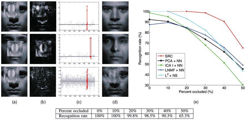
2 IEEE TRANSACTIONS ON PATTERN ANALYSIS AND MACHINE INTELLIGENCE, VOL. 31, NO. 2, FEBRUARY 2009
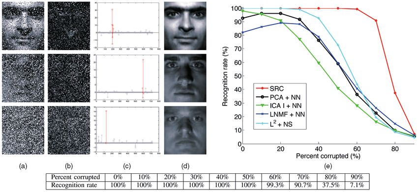
Fig. 1. Overview of our approach. Our method represents a test image (left), which is (a) potentially occluded or (b) corrupted, as a sparse linear
combination of all the training images (middle) plus sparse errors (right) due to occlusion or corruption. Red (darker) coefficients correspond to
training images of the correct individual. Our algorithm determines the true identity (indicated with a red box at second row and third column) from
700 training images of 100 individuals (7 each) in the standard AR face database.
[12], [14] penalizes the ‘1 -norm of the coefficients in the Our use of sparsity for classification differs significantly
linear combination, rather than the directly penalizing the from the various parsimony principles discussed above.
number of nonzero coefficients (i.e., the ‘0 -norm). Instead of using sparsity to identify a relevant model or
The original goal of these works was not inference or relevant features that can later be used for classifying all test
classification per se, but rather representation and compres- samples, it uses the sparse representation of each individual
sion of signals, potentially using lower sampling rates than test sample directly for classification, adaptively selecting
the Shannon-Nyquist bound [15]. Algorithm performance the training samples that give the most compact representa-
was therefore measured in terms of sparsity of the tion. The proposed classifier can be considered a general-
representation and fidelity to the original signals. Further- ization of popular classifiers such as nearest neighbor (NN)
more, individual base elements in the dictionary were not [18] and nearest subspace (NS) [19] (i.e., minimum distance to
assumed to have any particular semantic meaning—they the subspace spanned all training samples from each object
are typically chosen from standard bases (e.g., Fourier, class). NN classifies the test sample based on the best
Wavelet, Curvelet, and Gabor), or even generated from representation in terms of a single training sample, whereas
random matrices [11], [15]. Nevertheless, the sparsest NS classifies based on the best linear representation in
representation is naturally discriminative: among all subsets terms of all the training samples in each class. The nearest
of base vectors, it selects the subset which most compactly feature line (NFL) algorithm [20] strikes a balance between
expresses the input signal and rejects all other possible but these two extremes, classifying based on the best affine
less compact representations. representation in terms of a pair of training samples. Our
In this paper, we exploit the discriminative nature of method strikes a similar balance but considers all possible
supports (within each class or across multiple classes) and
sparse representation to perform classification. Instead of
adaptively chooses the minimal number of training samples
using the generic dictionaries discussed above, we repre-
needed to represent each test sample.3
sent the test sample in an overcomplete dictionary whose
We will motivate and study this new approach to
base elements are the training samples themselves. If sufficient
classification within the context of automatic face recogni-
training samples are available from each class,2 it will be
tion. Human faces are arguably the most extensively
possible to represent the test samples as a linear combina- studied object in image-based recognition. This is partly
tion of just those training samples from the same class. This due to the remarkable face recognition capability of the
representation is naturally sparse, involving only a small human visual system [21] and partly due to numerous
fraction of the overall training database. We argue that in important applications for face recognition technology [22].
many problems of interest, it is actually the sparsest linear In addition, technical issues associated with face recognition
representation of the test sample in terms of this dictionary are representative of object recognition and even data
and can be recovered efficiently via ‘1 -minimization. classification in general. Conversely, the theory of sparse
Seeking the sparsest representation therefore automatically representation and compressed sensing yields new insights
discriminates between the various classes present in the into two crucial issues in automatic face recognition: the
training set. Fig. 1 illustrates this simple idea using face role of feature extraction and the difficulty due to occlusion.
recognition as an example. Sparse representation also The role of feature extraction. The question of which low-
provides a simple and surprisingly effective means of dimensional features of an object image are the most relevant or
rejecting invalid test samples not arising from any class in informative for classification is a central issue in face recogni-
the training database: these samples’ sparsest representa- tion and in object recognition in general. An enormous
tions tend to involve many dictionary elements, spanning volume of literature has been devoted to investigate various
multiple classes. data-dependent feature transformations for projecting the
2. In contrast, methods such as that in [16] and [17] that utilize only a 3. The relationship between our method and NN, NS, and NFL is
single training sample per class face a more difficult problem and generally explored more thoroughly in the supplementary appendix, which can
incorporate more explicit prior knowledge about the types of variation that be found on the Computer Society Digital Library at http://
could occur in the test sample. doi.ieeecomputersociety.org/10.1109/TPAMI.2008.79.
WRIGHT ET AL.: ROBUST FACE RECOGNITION VIA SPARSE REPRESENTATION                                                                                   3

high-dimensional test image into lower dimensional feature           2     CLASSIFICATION BASED                  ON    SPARSE
spaces: examples include Eigenfaces [23], Fisherfaces [24],                REPRESENTATION
Laplacianfaces [25], and a host of variants [26], [27]. With so
many proposed features and so little consensus about which           A basic problem in object recognition is to use labeled
are better or worse, practitioners lack guidelines to decide         training samples from k distinct object classes to correctly
which features to use. However, within our proposed                  determine the class to which a new test sample belongs. We
framework, the theory of compressed sensing implies that             arrange the given ni training samples from the ith class as
                                                                                               :
the precise choice of feature space is no longer critical: Even      columns of a matrix Ai ¼½vvi;1 ; v i;2 ; . . . ; v i;ni  2 IRmni . In the
random features contain enough information to recover the            context of face recognition, we will identify a w  h gray-
sparse representation and hence correctly classify any test          scale image with the vector v 2 IRm ðm ¼ whÞ given by
image. What is critical is that the dimension of the feature         stacking its columns; the columns of Ai are then the training
space is sufficiently large and that the sparse representation       face images of the ith subject.
is correctly computed.
                                                                     2.1   Test Sample as a Sparse Linear Combination of
    Robustness to occlusion. Occlusion poses a significant
                                                                           Training Samples
obstacle to robust real-world face recognition [16], [28],
                                                                     An immense variety of statistical, generative, or discrimi-
[29]. This difficulty is mainly due to the unpredictable nature
                                                                     native models have been proposed for exploiting the
of the error incurred by occlusion: it may affect any part of
                                                                     structure of the Ai for recognition. One particularly simple
the image and may be arbitrarily large in magnitude.
                                                                     and effective approach models the samples from a single
Nevertheless, this error typically corrupts only a fraction of
                                                                     class as lying on a linear subspace. Subspace models are
the image pixels and is therefore sparse in the standard basis
                                                                     flexible enough to capture much of the variation in real data
given by individual pixels. When the error has such a sparse
                                                                     sets and are especially well motivated in the context of face
representation, it can be handled uniformly within our
                                                                     recognition, where it has been observed that the images of
framework: the basis in which the error is sparse can be
                                                                     faces under varying lighting and expression lie on a special
treated as a special class of training samples. The subsequent
                                                                     low-dimensional subspace [24], [30], often called a face
sparse representation of an occluded test image with respect
                                                                     subspace. Although the proposed framework and algorithm
to this expanded dictionary (training images plus error
                                                                     can also apply to multimodal or nonlinear distributions (see
basis) naturally separates the component of the test image
                                                                     the supplementary appendix for more detail, which can be
arising due to occlusion from the component arising from
                                                                     found on the Computer Society Digital Library at http://
the identity of the test subject (see Fig. 1 for an example). In     doi.ieeecomputersociety.org/10.1109/TPAMI.2008.79), for
this context, the theory of sparse representation and                ease of presentation, we shall first assume that the training
compressed sensing characterizes when such source-and-               samples from a single class do lie on a subspace. This is the
error separation can take place and therefore how much               only prior knowledge about the training samples we will be
occlusion the resulting recognition algorithm can tolerate.          using in our solution.4
    Organization of this paper. In Section 2, we introduce a basic      Given sufficient training samples of the ith object class,
general framework for classification using sparse represen-
                                                                     Ai ¼ ½vvi;1 ; v i;2 ; . . . ; v i;ni  2 IRmni , any new (test) sample y 2
tation, applicable to a wide variety of problems in image-
                                                                     IRm from the same class will approximately lie in the linear
based object recognition. We will discuss why the sparse
                                                                     span of the training samples5 associated with object i:
representation can be computed by ‘1 -minimization and
how it can be used for classifying and validating any given                         y ¼ i;1 v i;1 þ i;2 v i;2 þ    þ i;ni v i;ni ;         ð1Þ
test sample. Section 3 shows how to apply this general
classification framework to study two important issues in            for some scalars, i;j 2 IR, j ¼ 1; 2; . . . ; ni .
                                                                        Since the membership i of the test sample is initially
image-based face recognition: feature extraction and robust-
                                                                     unknown, we define a new matrix A for the entire training
ness to occlusion. In Section 4, we verify the proposed
                                                                     set as the concatenation of the n training samples of all
method with extensive experiments on popular face data
                                                                     k object classes:
sets and comparisons with many other state-of-the-art face
recognition techniques. Further connections between our                           :
                                                                                A¼½A1 ; A2 ; . . . ; Ak  ¼ ½vv1;1 ; v 1;2 ; . . . ; v k;nk : ð2Þ
method, NN, and NS are discussed in the supplementary
appendix, which can be found on the Computer Society                 Then, the linear representation of y can be rewritten in
Digital Library at http://doi.ieeecomputersociety.org/               terms of all training samples as
10.1109/TPAMI.2008.79.                                                                           y ¼ Ax
                                                                                                      x0         2 IRm ;                         ð3Þ
    While the proposed method is of broad interest to object
                                                                                                                                       T   n
recognition in general, the studies and experimental results         where x 0 ¼ ½0;    ; 0; i;1 ; i;2 ; . . . ; i;ni ; 0; . . . ; 0 2 IR is a
in this paper are confined to human frontal face recognition.        coefficient vector whose entries are zero except those
We will deal with illumination and expressions, but we do            associated with the ith class.
not explicitly account for object pose nor rely on any
                                                                         4. In face recognition, we actually do not need to know whether the
3D model of the face. The proposed algorithm is robust to            linear structure is due to varying illumination or expression, since we do
small variations in pose and displacement, for example, due          not rely on domain-specific knowledge such as an illumination model [31]
to registration errors. However, we do assume that detec-            to eliminate the variability in the training and testing images.
                                                                         5. One may refer to [32] for how to choose the training images to ensure
tion, cropping, and normalization of the face have been              this property for face recognition. Here, we assume that such a training set
performed prior to applying our algorithm.                           is given.
4                                    IEEE TRANSACTIONS ON PATTERN ANALYSIS AND MACHINE INTELLIGENCE,                 VOL. 31, NO. 2,    FEBRUARY 2009

    As the entries of the vector x 0 encode the identity of the
test sample y, it is tempting to attempt to obtain it by
solving the linear system of equations y ¼ Ax       x. Notice,
though, that using the entire training set to solve for x
represents a significant departure from one sample or one
class at a time methods such as NN and NS. We will later
argue that one can obtain a more discriminative classifier
from such a global representation. We will demonstrate its
superiority over these local methods (NN or NS) both for
identifying objects represented in the training set and for
rejecting outlying samples that do not arise from any of the                  Fig. 2. Geometry of sparse representation via ‘1 -minimization. The
classes present in the training set. These advantages can                     ‘1 -minimization determines which facet (of the lowest dimension) of the
come without an increase in the order of growth of the                        polytope AðP Þ, the point y=kyyk1 lies in. The test sample vector y is
computation: As we will see, the complexity remains linear                    represented as a linear combination of just the vertices of that facet, with
                                                                              coefficients x0 .
in the size of training set.
    Obviously, if m > n, the system of equations y ¼ Ax    x is
overdetermined, and the correct x 0 can usually be found as                   that if the solution x0 sought is sparse enough, the solution of
its unique solution. We will see in Section 3, however, that                  the ‘0 -minimization problem (5) is equal to the solution to
in robust face recognition, the system y ¼ Ax    x is typically               the following ‘1 -minimization problem:
underdetermined, and so, its solution is not unique.6
Conventionally, this difficulty is resolved by choosing the                        ð‘1 Þ :     ^ 1 ¼ arg min kx
                                                                                               x              xk1                   x ¼ y:
                                                                                                                        subject to Ax                 ð6Þ
minimum ‘2 -norm solution:                                                    This problem can be solved in polynomial time by standard
                                                                              linear programming methods [34]. Even more efficient
    ð‘2 Þ :      ^ 2 ¼ arg min kx
                 x              xk 2     subject to      x ¼ y:
                                                        Ax             ð4Þ    methods are available when the solution is known to be
While this optimization problem can be easily solved (via                     very sparse. For example, homotopy algorithms recover
the pseudoinverse of A), the solution x     ^ 2 is not especially             solutions with t nonzeros in Oðt3 þ nÞ time, linear in the size
informative for recognizing the test sample y . As shown in                   of the training set [35].
Example 1, x ^ 2 is generally dense, with large nonzero entries
corresponding to training samples from many different                         2.2.1 Geometric Interpretation
classes. To resolve this difficulty, we instead exploit the                   Fig. 2 gives a geometric interpretation (essentially due to
following simple observation: A valid test sample y can be                    [36]) of why minimizing the ‘1 -norm correctly recovers
sufficiently represented using only the training samples                      sufficiently sparse solutions. Let P denote the ‘1 -ball (or
from the same class. This representation is naturally sparse if               crosspolytope) of radius :
the number of object classes k is reasonably large. For                                           :
                                                                                               P ¼fx    xk1  g  IRn :
                                                                                                    x : kx                              ð7Þ
instance, if k ¼ 20, only 5 percent of the entries of the
desired x 0 should be nonzero. The more sparse the                            In Fig. 2, the unit ‘1 -ball P1 is mapped to the polytope
recovered x 0 is, the easier will it be to accurately determine                   :
                                                                              P ¼AðP1 Þ  IRm , consisting of all y that satisfy y ¼ Ax      x for
the identity of the test sample y .7                                          some x whose ‘1 -norm is  1.
   This motivates us to seek the sparsest solution to y ¼ Ax   x,                  The geometric relationship between P and the polytope
solving the following optimization problem:                                   AðP Þ is invariant to scaling. That is, if we scale P , its
                                                                              image under multiplication by A is also scaled by the same
    ð‘0 Þ :      ^ 0 ¼ arg min kx
                 x              xk 0     subject to      x ¼ y;
                                                        Ax             ð5Þ    amount. Geometrically, finding the minimum ‘1 -norm
                                0
where k  k0 denotes the ‘ -norm, which counts the number                     solution x ^ 1 to (6) is equivalent to expanding the ‘1 -ball P
of nonzero entries in a vector. In fact, if the columns of A are              until the polytope AðP Þ first touches y. The value of  at
in general position, then whenever y ¼ Ax     x for some x with               which this occurs is exactly k^     x 1 k1 .
less than m=2 nonzeros, x is the unique sparsest solution:                         Now, suppose that y ¼ Ax     x0 for some sparse x 0 . We wish
^ 0 ¼ x [33]. However, the problem of finding the sparsest
x                                                                             to know when solving (6) correctly recovers x 0 . This
solution of an underdetermined system of linear equations is                  question is easily resolved from the geometry of that in
NP-hard and difficult even to approximate [13]: that is, in the               Fig. 2: Since x ^ 1 is found by expanding both P and AðP Þ
general case, no known procedure for finding the sparsest                     until a point of AðP Þ touches y , the ‘1 -minimizer x    ^ 1 must
solution is significantly more efficient than exhausting all                  generate a point A^     x 1 on the boundary of P .
subsets of the entries for x .                                                           ^ 1 ¼ x 0 if and only if the point Aðx
                                                                                   Thus, x                                         x0 k1 Þ lies on
                                                                                                                              x0 =kx
                                                                              the boundary of the polytope P . For the example shown in
2.2 Sparse Solution via ‘1 -Minimization                                      Fig. 2, it is easy to see that the ‘1 -minimization recovers all
Recent development in the emerging theory of sparse                           x0 with only one nonzero entry. This equivalence holds
representation and compressed sensing [9], [10], [11] reveals                 because all of the vertices of P1 map to points on the
                                                                              boundary of P .
   6. Furthermore, even in the overdetermined case, such a linear equation
may not be perfectly satisfied in the presence of data noise (see                  In general, if A maps all t-dimensional facets of P1 to
Section 2.2.2).                                                               facets of P , the polytope P is referred to as (centrally)
   7. This intuition holds only when the size of the database is fixed. For   t-neighborly [36]. From the above, we see that the
example, if we are allowed to append additional irrelevant columns to A,
we can make the solution x0 have a smaller fraction of nonzeros, but this     ‘1 -minimization (6) correctly recovers all x 0 with  t þ 1
does not make x0 more informative for recognition.                            nonzeros if and only if P is t-neighborly, in which case, it is
WRIGHT ET AL.: ROBUST FACE RECOGNITION VIA SPARSE REPRESENTATION                                                                                           5

Fig. 3. A valid test image. (a) Recognition with 12  10 downsampled images as features. The test image y belongs to subject 1. The values of the
sparse coefficients recovered from Algorithm 1 are plotted on the right together with the two training examples that correspond to the two largest
                                                                                                                                  xÞ by ‘1 -minimization. The
sparse coefficients. (b) The residuals ri ðyyÞ of a test image of subject 1 with respect to the projected sparse coefficients i ð^
ratio between the two smallest residuals is about 1:8.6.

equivalent to the ‘0 -minimization (5).8 This condition is                      2.3 Classification Based on Sparse Representation
surprisingly common: even polytopes P given by random                           Given a new test sample y from one of the classes in the
matrices (e.g., uniform, Gaussian, and partial Fourier) are                     training set, we first compute its sparse representation x      ^1
highly neighborly [15], allowing correct recover of sparse x 0                  via (6) or (10). Ideally, the nonzero entries in the estimate x ^1
by ‘1 -minimization.                                                            will all be associated with the columns of A from a single
   Unfortunately, there is no known algorithm for effi-                         object class i, and we can easily assign the test sample y to
ciently verifying the neighborliness of a given polytope P .                    that class. However, noise and modeling error may lead to
The best known algorithm is combinatorial, and therefore,                       small nonzero entries associated with multiple object
only practical when the dimension m is moderate [37].                           classes (see Fig. 3). Based on the global sparse representa-
When m is large, it is known that with overwhelming                             tion, one can design many possible classifiers to resolve
probability, the neighborliness of a randomly chosen                            this. For instance, we can simply assign y to the object class
polytope P is loosely bounded between                                           with the single largest entry in x  ^ 1 . However, such heuristics
                                                                                do not harness the subspace structure associated with
                      c  m < t < bðm þ 1Þ=3c;                           ð8Þ
                                                                                images in face recognition. To better harness such linear
for some small constant c > 0 (see [9] and [36]). Loosely                       structure, we instead classify y based on how well the
speaking, as long as the number of nonzero entries of x 0 is a                  coefficients associated with all training samples of each
small fraction of the dimension m, ‘1 -minimization will                        object reproduce y .
recover x 0 .                                                                       For each class i, let i : IRn ! IRn be the characteristic
                                                                                function that selects the coefficients associated with the
2.2.2 Dealing with Small Dense Noise                                            ith class. For x 2 IRn , i ðx
                                                                                                             xÞ 2 IRn is a new vector whose only
So far, we have assumed that (3) holds exactly. Since real                      nonzero entries are the entries in x that are associated with
data are noisy, it may not be possible to express the test                      class i. Using only the coefficients associated with the
sample exactly as a sparse superposition of the training                        ith class, one can approximate the given test sample y as
samples. The model (3) can be modified to explicitly                            y^i ¼ Ai ð^
                                                                                           x 1 Þ. We then classify y based on these approxima-
account for small possibly dense noise by writing                               tions by assigning it to the object class that minimizes the
                                   x0 þ z ;
                              y ¼ Ax                                     ð9Þ    residual between y and y^i :
                                                                                                                :
                 m
where z 2 IR is a noise term with bounded energy                                                    min ri ðyyÞ¼kyy  A i ð^
                                                                                                                            x 1 Þk2 :        ð12Þ
                                                                                                        i
kzzk2 < ". The sparse solution x 0 can still be approximately
recovered by solving the following stable ‘1 -minimization                      Algorithm 1 below summarizes the complete recognition
problem:                                                                        procedure. Our implementation minimizes the ‘1 -norm via
                                                                                a primal-dual algorithm for linear programming based on
   ð‘1s Þ :   ^ 1 ¼ arg min kx
              x              xk 1     subject to     kAx
                                                       x  y k2  ":            [39] and [40].
                                                                       ð10Þ     Algorithm 1. Sparse Representation-based Classification
    This convex optimization problem can be efficiently                         (SRC)
solved via second-order cone programming [34] (see                               1: Input: a matrix of training samples
Section 4 for our algorithm of choice). The solution of ð‘1s Þ                      A ¼ ½A1 ; A2 ; . . . ; Ak  2 IRmn for k classes, a test sample
is guaranteed to approximately recovery sparse solutions in                         y 2 IRm , (and an optional error tolerance " > 0.)
ensembles of random matrices A [38]: There are constants                        2: Normalize the columns of A to have unit ‘2 -norm.
and  such that with overwhelming probability, if kx x0 k 0 <
                                                                                 3: Solve the ‘1 -minimization problem:
m and kzzk2  ", then the computed x^ 1 satisfies
                                                                                               ^ 1 ¼ arg minx kx
                                                                                               x                    xk1 subject to Ax x ¼ y:     ð13Þ
                            k^
                             x 1  x 0 k2  ":                        ð11Þ         (Or alternatively, solve
                                                                                               ^ 1 ¼ arg minx kx
                                                                                               x                    xk1 subject to kAx x yyk2  ":Þ
   8. Thus, neighborliness gives a necessary and sufficient condition for        4: Compute the residuals ri ðyyÞ ¼ kyy  A i ð^    x 1 Þk2
sparse recovery. The restricted isometry properties often used in analyzing
the performance of ‘1 -minimization in random matrix ensembles (e.g., [15])                    for i ¼ 1; . . . ; k.
give sufficient, but not necessary, conditions.                                  5: Output: identityðyyÞ ¼ arg mini ri ðyyÞ.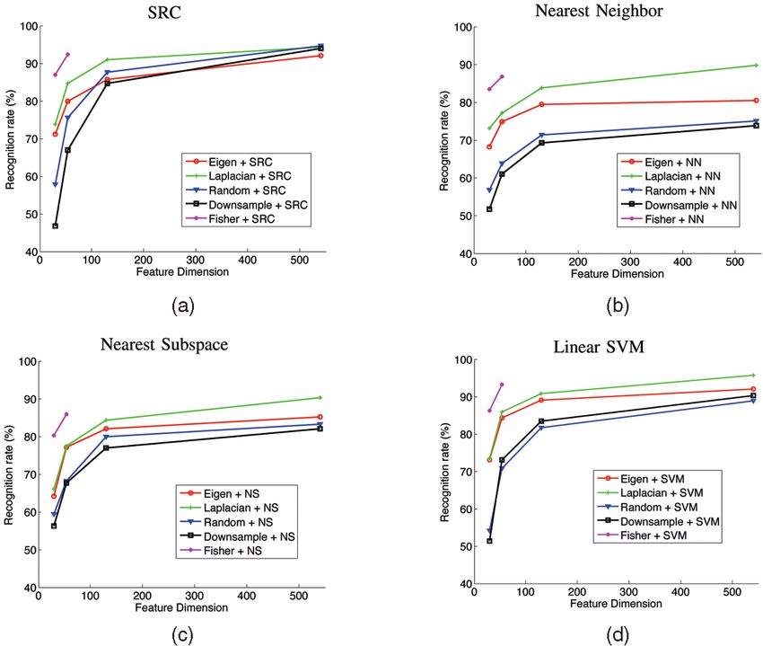
6                                   IEEE TRANSACTIONS ON PATTERN ANALYSIS AND MACHINE INTELLIGENCE,                  VOL. 31, NO. 2,    FEBRUARY 2009

Fig. 4. Nonsparsity of the ‘2 -minimizer. (a) Coefficients from ‘2 -minimization using the same test image as Fig. 3. The recovered solution is not
sparse and, hence, less informative for recognition (large coefficients do not correspond to training images of this test subject). (b) The residuals of
                                                                 xÞ of the coefficients obtained by ‘2 -minimization. The ratio between the two smallest
the test image from subject 1 with respect to the projection i ð^
residuals is about 1:1.3. The smallest residual is not associated with subject 1.

Example 1 (‘1 -minimization versus ‘2 -minimization). To                     test sample based on how small the smallest residual is.
  illustrate how Algorithm 1 works, we randomly select                       However, each residual ri ðyyÞ is computed without any
  half of the 2,414 images in the Extended Yale B database                   knowledge of images of other object classes in the training
  as the training set and the rest for testing. In this                      data set and only measures similarity between the test
  example, we subsample the images from the original 192                     sample and each individual class.
   168 to size 12  10. The pixel values of the                                In the sparse representation paradigm, the coefficients x ^1
  downsampled image are used as 120-D feature-                               are computed globally, in terms of images of all classes. In a
  s—stacked as columns of the matrix A in the algorithm.                     sense, it can harness the joint distribution of all classes for
  Hence, matrix A has size 120  1,207, and the system                       validation. We contend that the coefficients x   ^ are better
  y ¼ Ax x is underdetermined. Fig. 3a illustrates the sparse                statistics for validation than the residuals. Let us first see
  coefficients recovered by Algorithm 1 for a test image                     this through an example.
  from the first subject. The figure also shows the features
  and the original images that correspond to the two                         Example 2 (concentration of sparse coefficients). We
  largest coefficients. The two largest coefficients are both                  randomly select an irrelevant image from Google and
  associated with training samples from subject 1. Fig. 3b                     downsample it to 12  10. We then compute the sparse
  shows the residuals with respect to the 38 projected                         representation of the image against the same Extended
  coefficients i ð^
                   x 1 Þ, i ¼ 1; 2; . . . ; 38. With 12  10 down-             Yale B training data, as in Example 1. Fig. 5a plots the
  sampled images as features, Algorithm 1 achieves an                          obtained coefficients, and Fig. 5b plots the corresponding
  overall recognition rate of 92.1 percent across the                          residuals. Compared to the coefficients of a valid test
  Extended Yale B database. (See Section 4 for details                         image in Fig. 3, notice that the coefficients x
                                                                                                                             ^ here are not
  and performance with other features such as Eigenfaces                       concentrated on any one subject and instead spread
  and Fisherfaces, as well as comparison with other                            widely across the entire training set. Thus, the distribu-
  methods.) Whereas the more conventional minimum                              tion of the estimated sparse coefficients x      ^ contains
  ‘2 -norm solution to the underdetermined system y ¼ Ax         x             important information about the validity of the test
  is typically quite dense, minimizing the ‘1 -norm favors                     image: a valid test image should have a sparse
  sparse solutions and provably recovers the sparsest                          representation whose nonzero entries concentrate mostly
  solution when this solution is sufficiently sparse. To                       on one subject, whereas an invalid image has sparse
  illustrate this contrast, Fig. 4a shows the coefficients of                  coefficients spread widely among multiple subjects.
  the same test image given by the conventional
  ‘2 -minimization (4), and Fig. 4b shows the corresponding                     To quantify this observation, we define the following
  residuals with respect to the 38 subjects. The coefficients                measure of how concentrated the coefficients are on a single
  are much less sparse than those given by ‘1 -minimization                  class in the data set:
  (in Fig. 3), and the dominant coefficients are not                         Definition 1 (sparsity concentration index (SCI)). The SCI
  associated with subject 1. As a result, the smallest                         of a coefficient vector x 2 IRn is defined as
  residual in Fig. 4 does not correspond to the correct
  subject (subject 1).                                                                    : k  maxi ki ðx
                                                                                                          xÞk1 =kx
                                                                                                                 xk1  1
                                                                                        xÞ¼
                                                                                    SCIðx                                           2 ½0; 1:       ð14Þ
                                                                                                       k1
2.4 Validation Based on Sparse Representation
Before classifying a given test sample, we must first decide                 For a solution x^ found by Algorithm 1, if SCIð^    x Þ ¼ 1, the
if it is a valid sample from one of the classes in the data set.             test image is represented using only images from a single
The ability to detect and then reject invalid test samples, or                                  x Þ ¼ 0, the sparse coefficients are spread
                                                                             object, and if SCIð^
“outliers,” is crucial for recognition systems to work in real-              evenly over all classes.9 We choose a threshold  2 ð0; 1Þ
world situations. A face recognition system, for example,                    and accept a test image as valid if
could be given a face image of a subject that is not in the
database or an image that is not a face at all.                                 9. Directly choosing x to minimize the SCI might produce more
                                                                             concentrated coefficients; however, the SCI is highly nonconvex and
    Systems based on conventional classifiers such as NN or                  difficult to optimize. For valid test images, minimizing the ‘0 -norm already
NS, often use the residuals ri ðyyÞ for validation, in addition              produces representations that are well-concentrated on the correct subject
to identification. That is, the algorithm accepts or rejects a               class.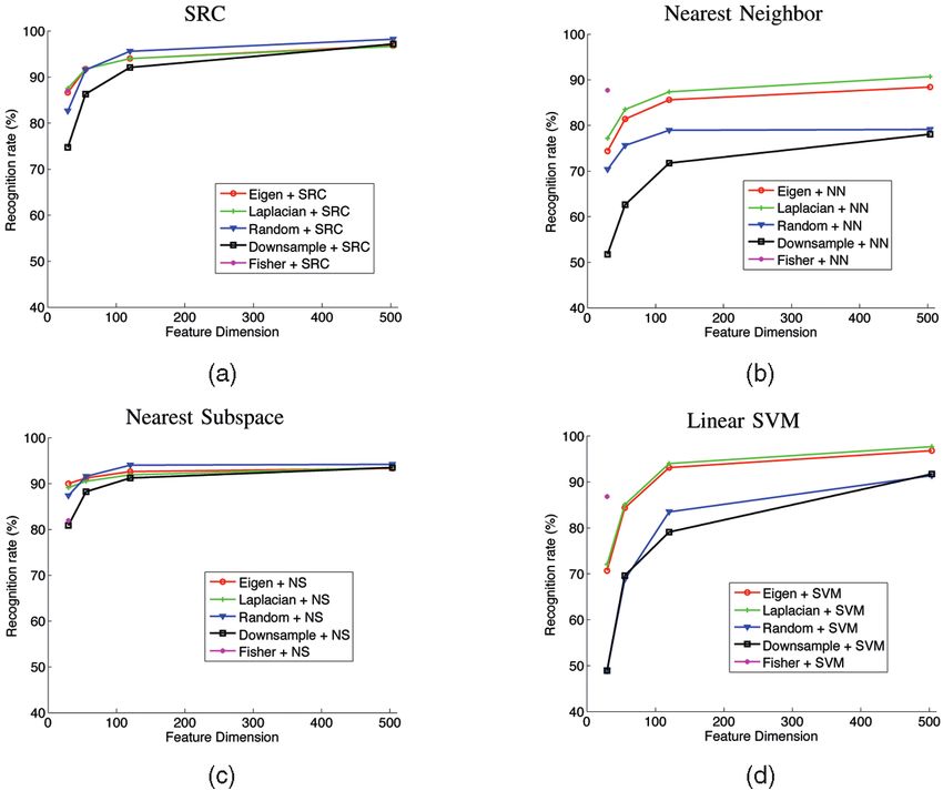
WRIGHT ET AL.: ROBUST FACE RECOGNITION VIA SPARSE REPRESENTATION                                                                                     7

Fig. 5. Example of an invalid test image. (a) Sparse coefficients for the invalid test image with respect to the same training data set from
Example 1. The test image is a randomly selected irrelevant image. (b) The residuals of the invalid test image with respect to the projection i ð^
                                                                                                                                                  xÞ of
the sparse representation computed by ‘1 -minimization. The ratio of the two smallest residuals is about 1:1.2.

                                  xÞ
                              SCIð^       ;                          ð15Þ     3.1 The Role of Feature Extraction
and otherwise reject as invalid. In step 5 of Algorithm 1, one                 In the computer vision literature, numerous feature extrac-
may choose to output the identity of y only if it passes this                  tion schemes have been investigated for finding projections
criterion.                                                                     that better separate the classes in lower dimensional spaces,
   Unlike NN or NS, this new rule avoids the use of the                        which are often referred to as feature spaces. One class of
residuals ri ðyyÞ for validation. Notice that in Fig. 5, even for a            methods extracts holistic face features such as Eigen-
nonface image, with a large training set, the smallest                         faces[23], Fisherfaces [24], and Laplacianfaces [25]. Another
residual of the invalid test image is not so large. Rather                     class of methods tries to extract meaningful partial facial
than relying on a single statistic for both validation and                     features (e.g., patches around eyes or nose) [21], [41] (see
identification, our approach separates the information                         Fig. 6 for some examples). Traditionally, when feature
required for these tasks: the residuals for identification                     extraction is used in conjunction with simple classifiers
and the sparse coefficients for validation.10 In a sense, the                  such as NN and NS, the choice of feature transformation is
residual measures how well the representation approx-                          considered critical to the success of the algorithm. This has
imates the test image; and the sparsity concentration index                    led to the development of a wide variety of increasingly
measures how good the representation itself is, in terms of                    complex feature extraction methods, including nonlinear
localization.                                                                  and kernel features [42], [43]. In this section, we reexamine
   One benefit to this approach to validation is improved                      the role of feature extraction within the new sparse
performance against generic objects that are similar to                        representation framework for face recognition.
multiple object classes. For example, in face recognition, a                      One benefit of feature extraction, which carries over to
generic face might be rather similar to some of the                            the proposed sparse representation framework, is reduced
subjects in the data set and may have small residuals                          data dimension and computational cost. For raw face
with respect to their training images. Using residuals for                     images, the corresponding linear system y ¼ Ax        x is very
validation more likely leads to a false positive. However,                     large. For instance, if the face images are given at the typical
a generic face is unlikely to pass the new validation rule                     resolution, 640  480 pixels, the dimension m is in the order
as a good representation of it typically requires contribu-                    of 105 . Although Algorithm 1 relies on scalable methods
tion from images of multiple subjects in the data set.                         such as linear programming, directly applying it to such
Thus, the new rule can better judge whether the test
                                                                               high-resolution images is still beyond the capability of
image is a generic face or the face of one particular
                                                                               regular computers.
subject in the data set. In Section 4.7, we will demonstrate
                                                                                  Since most feature transformations involve only linear
that the new validation rule outperforms the NN and NS
methods, with as much as 10-20 percent improvement in                          operations (or approximately so), the projection from the
verification rate for a given false accept rate (see Fig. 14                   image space to the feature space can be represented as a
in Section 4 or Fig. 18 in the supplementary appendix,                         matrix R 2 IRdm with d        m. Applying R to both sides of
which can be found on the Computer Society Digital                             (3) yields
Library at http://doi.ieeecomputersociety.org/10.1109/                                                 :
TPAMI.2008.79).                                                                                     y~ ¼ Ryy ¼ RAx
                                                                                                                 x0      2 IRd :                  ð16Þ
                                                                               In practice, the dimension d of the feature space is typically
3    TWO FUNDAMENTAL ISSUES                    IN   FACE                       chosen to be much smaller than n. In this case, the system of
                                                                               equations y~ ¼ RAx  x 2 IRd is underdetermined in the un-
     RECOGNITION                                                                              n
                                                                               known x 2 IR . Nevertheless, as the desired solution x 0 is
In this section, we study the implications of the above                        sparse, we can hope to recover it by solving the following
general classification framework for two critical issues in                    reduced ‘1 -minimization problem:
face recognition: 1) the choice of feature transformation, and
2) robustness to corruption, occlusion, and disguise.                            ð‘1r Þ :   ^ 1 ¼ arg min kx
                                                                                            x              xk1   subject to    kRAx
                                                                                                                                  x  y~k2  ";
   10. We find empirically that this separation works well enough in our
                                                                                                                                                  ð17Þ
experiments with face images. However, it is possible that better validation
and identification rules can be contrived from using the residual and the      for a given error tolerance " > 0. Thus, in Algorithm 1, the
sparsity together.                                                             matrix A of training images is now replaced by the matrix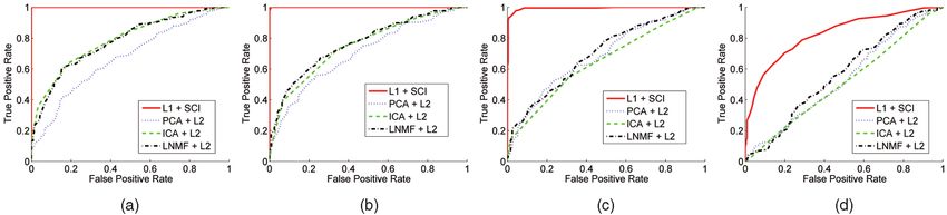
8                                     IEEE TRANSACTIONS ON PATTERN ANALYSIS AND MACHINE INTELLIGENCE,                      VOL. 31, NO. 2,    FEBRUARY 2009

Fig. 6. Examples of feature extraction. (a) Original face image. (b) 120D representations in terms of four different features (from left to right):
Eigenfaces, Laplacianfaces, downsampled (12  10 pixel) image, and random projection. We will demonstrate that all these features contain almost
the same information about the identity of the subject and give similarly good recognition performance. (c) The eye is a popular choice of feature for
face recognition. In this case, the feature matrix R is simply a binary mask. (a) Original y. (b) 120D features y~ ¼ Ryy. (c) Eye feature~y .

RA 2 IRdn of d-dimensional features; the test image y is                        random linear measurements are sufficient for ‘1 -minimiza-
replaced by its features y~.                                                     tion (17) to recover the correct sparse solution x0 [44].12 This
    For extant face recognition methods, empirical studies                       surprising phenomenon has been dubbed the “blessing of
have shown that increasing the dimension d of the feature                        dimensionality” [15], [46]. Random features can be viewed
space generally improves the recognition rate, as long as the                    as a less-structured counterpart to classical face features
distribution of features RAi does not become degenerate                          such as Eigenfaces or Fisherfaces. Accordingly, we call the
[42]. Degeneracy is not an issue for ‘1 -minimization, since it                  linear projection generated by a Gaussian random matrix
merely requires that y~ be in or near the range of RAi —it                       Randomfaces.13
does not depend on the covariance i ¼ ATi RT RAi being                          Definition 2 (randomfaces). Consider a transform matrix R 2
nonsingular as in classical discriminant analysis. The stable                      IRdm whose entries are independently sampled from a zero-
version of ‘1 -minimization (10) or (17) is known in statistical                   mean normal distribution, and each row is normalized to unit
literature as the Lasso [14].11 It effectively regularizes highly                  length. The row vectors of R can be viewed as d random faces
underdetermined linear regression when the desired solu-                           in IRm .
tion is sparse and has also been proven consistent in some
noisy overdetermined settings [12].                                                 One major advantage of Randomfaces is that they are
                                                                                 extremely efficient to generate, as the transformation R is
    For our sparse representation approach to recognition, we
                                                                                 independent of the training data set. This advantage can be
would like to understand how the choice of the feature                           important for a face recognition system, where we may not
extraction R affects the ability of the ‘1 -minimization (17) to                 be able to acquire a complete database of all subjects of
recover the correct sparse solution x 0 . From the geometric                     interest to precompute data-dependent transformations
interpretation of ‘1 -minimization given in Section 2.2.1, the                   such as Eigenfaces, or the subjects in the database may
answer to this depends on whether the associated new                             change over time. In such cases, there is no need for
polytope P ¼ RAðP1 Þ remains sufficiently neighborly. It is                      recomputing the random transformation R.
                                                                                    As long as the correct sparse solution x 0 can be
easy to show that the neighborliness of the polytope P ¼
                                                                                 recovered, Algorithm 1 will always give the same classifica-
RAðP1 Þ increases with d [11], [15]. In Section 4, our                           tion result, regardless of the feature actually used. Thus,
experimental results will verify the ability of ‘1 -minimiza-                    when the dimension of feature d exceeds the above bound
tion, in particular, the stable version (17), to recover sparse                  (18), one should expect that the recognition performance of
representations for face recognition using a variety of                          Algorithm 1 with different features quickly converges, and
features. This suggests that most data-dependent features                        the choice of an “optimal” feature transformation is no
popular in face recognition (e.g., eigenfaces and Laplacian-                     longer critical: even random projections or downsampled
                                                                                 images should perform as well as any other carefully
faces) may indeed give highly neighborly polytopes P .
                                                                                 engineered features. This will be corroborated by the
    Further analysis of high-dimensional polytope geometry                       experimental results in Section 4.
has revealed a somewhat surprising phenomenon: if the
solution x0 is sparse enough, then with overwhelming                             3.2 Robustness to Occlusion or Corruption
probability, it can be correctly recovered via ‘1 -minimization                  In many practical face recognition scenarios, the test image
from any sufficiently large number d of linear measurements                      y could be partially corrupted or occluded. In this case, the
y~ ¼ RAx x0 . More precisely, if x 0 has t      n nonzeros, then                 above linear model (3) should be modified as
with overwhelming probability                                                                           y ¼ y0 þ e0 ¼ A x0 þ e0 ;                          ð19Þ
                             d    2t logðn=dÞ                           ð18Þ
                                                                                    12. Strictly speaking, this threshold holds when random measurements
                                                                                 are computed directly from x0 , i.e., y~ ¼ Rxx0 . Nevertheless, our experiments
    11. Classically, the Lasso solution is defined as the minimizer of           roughly agree with the bound given by (18). The case where x0 is instead
kyy  Axxk22 þ kx
                 xk1 . Here,  can be viewed as inverse of the Lagrange          sparse in some overcomplete basis A, and we observe that random
                                               xk22  ". For every , there is
multiplier associated with a constraint kyy  Ax                                 measurements y~ ¼ R Ax    x0 has also been studied in [45]. While conditions for
an " such that the two problems have the same solution. However, " can be        correct recovery have been given, the bounds are not yet as sharp as (18)
interpreted as a pixel noise level and fixed across various instances of the     above.
problem, whereas  cannot. One should distinguish the Lasso optimization            13. Random projection has been previously studied as a general
problem from the LARS algorithm, which provably solves some instances of         dimensionality-reduction method for numerous clustering problems [47],
Lasso with very sparse optimizers [35].                                          [48], [49], as well as for learning nonlinear manifolds [50], [51].
WRIGHT ET AL.: ROBUST FACE RECOGNITION VIA SPARSE REPRESENTATION                                                                                   9

where e0 2 IRm is a vector of errors—a fraction, , of its                                                         x :
                                                                                                      y ¼ ½ A; I  0 ¼B w 0 :                   ð20Þ
entries are nonzero. The nonzero entries of e 0 model which                                                        e0
pixels in y are corrupted or occluded. The locations of                         Here, B ¼ ½A; I 2 IRmðnþmÞ , so the system y ¼ Bw          w is
corruption can differ for different test images and are not                     always underdetermined and does not have a unique
known to the computer. The errors may have arbitrary                            solution for w. However, from the above discussion about
magnitude and therefore cannot be ignored or treated with                       the sparsity of x 0 and e0 , the correct generating w0 ¼ ½xx0 ; e 0
techniques designed for small noise such as the one given in                    has at most ni þ m nonzeros. We might therefore hope to
Section 2.2.2.                                                                  recover w 0 as the sparsest solution to the system y ¼ Bw    w. In
   A fundamental principle of coding theory [52] is that                        fact, if the matrix B is in general position, then as long as
redundancy in the measurement is essential to detecting and                     y ¼ Bw  ~ for some w ~ with less than m=2 nonzeros, w   ~ is the
correcting gross errors. Redundancy arises in object recogni-                   unique sparsest solution. Thus, if the occlusion e covers less
tion because the number of image pixels is typically far                        than mn   i
                                                                                             pixels,  50 percent of the image, the sparsest
                                                                                         2
greater than the number of subjects that have generated the                     solution w ~ to y ¼ Bww is the true generator, w0 ¼ ½x x0 ; e0 .
images. In this case, even if a fraction of the pixels are                         More generally, one can assume that the corrupting error
completely corrupted by occlusion, recognition may still be                     e0 has a sparse representation with respect to some basis
possible based on the remaining pixels. On the other hand,                      Ae 2 IRmne . That is, e0 ¼ Ae u 0 for some sparse vector
feature extraction schemes discussed in the previous section                    u0 2 IRm . Here, we have chosen the special case Ae ¼ I 2
would discard useful information that could help compen-                        IRmm as e0 is assumed to be sparse with respect to the
sate for the occlusion. In this sense, no representation is more
                                                                                natural pixel coordinates. If the error e 0 is instead more
redundant, robust, or informative than the original images.
                                                                                sparse with respect to another basis, e.g., Fourier or Haar,
Thus, when dealing with occlusion and corruption, we
                                                                                we can simply redefine the matrix B by appending Ae
should always work with the highest possible resolution,
                                                                                (instead of the identity I) to A and instead seek the sparsest
performing downsampling or feature extraction only if the
                                                                                solution w0 to the equation:
resolution of the original images is too high to process.
   Of course, redundancy would be of no use without                                           y ¼ Bw
                                                                                                   w with B ¼ ½A; Ae        2 IRmðnþne Þ :    ð21Þ
efficient computational tools for exploiting the information
encoded in the redundant data. The difficulty in directly                       In this way, the same formulation can handle more general
harnessing the redundancy in corrupted raw images has led                       classes of (sparse) corruption.
researchers to instead focus on spatial locality as a guiding                      As before, we attempt to recover the sparsest solution
principle for robust recognition. Local features computed                       w0 from solving the following extended ‘1 -minimization
from only a small fraction of the image pixels are clearly less                 problem:
likely to be corrupted by occlusion than holistic features. In
face recognition, methods such as ICA [53] and LNMF [54]                           ð‘1e Þ :      ^ 1 ¼ arg min kw
                                                                                                 w              wk1    subject to    w ¼ y:
                                                                                                                                    Bw          ð22Þ
exploit this observation by adaptively choosing filter bases                    That is, in Algorithm 1, we now replace the image matrix A
that are locally concentrated. Local Binary Patterns [55] and                   with the extended matrix B ¼ ½A; I and x with w ¼ ½x   x; e.
Gabor wavelets [56] exhibit similar properties, since they are                     Clearly, whether the sparse solution w 0 can be recovered
also computed from local image regions. A related approach                      from the above ‘1 -minimization depends on the neighborli-
partitions the image into fixed regions and computes                            ness of the new polytope P ¼ BðP1 Þ ¼ ½A; IðP1 Þ. This
features for each region [16], [57]. Notice, though, that                       polytope contains vertices from both the training images
projecting onto locally concentrated bases transforms the                       A and the identity matrix I, as illustrated in Fig. 7. The
domain of the occlusion problem, rather than eliminating the                    bounds given in (8) imply that if y is an image of subject i,
occlusion. Errors on the original pixels become errors in the                   the ‘1 -minimization (22) cannot guarantee to correctly
transformed domain and may even become less local. The                          recover w0 ¼ ½xx0 ; e0  if
role of feature extraction in achieving spatial locality is
therefore questionable, since no bases or features are more                                           ni þ jsupportðee0 Þj > d=3:
spatially localized than the original image pixels themselves. In               Generally, d    ni , so, (8) implies that the largest fraction of
fact, the most popular approach to robustifying feature-                        occlusion under which we can hope to still achieve perfect
based methods is based on randomly sampling individual                          reconstruction is 33 percent. This bound is corroborated by
pixels [28], sometimes in conjunction with statistical                          our experimental results, see Fig. 12.
techniques such as multivariate trimming [29].                                     To know exactly how much occlusion can be tolerated,
   Now, let us show how the proposed sparse represen-                           we need more accurate information about the neighborli-
tation classification framework can be extended to deal                         ness of the polytope P than a loose upper bound given by
with occlusion. Let us assume that the corrupted pixels                         (8). For instance, we would like to know for a given set of
are a relatively small portion of the image. The error                          training images, what is the largest amount of (worst
vector e 0 , like the vector x 0 , then has sparse14 nonzero                    possible) occlusion it can handle. While the best known
entries. Since y 0 ¼ Ax x0 , we can rewrite (19) as                             algorithms for exactly computing the neighborliness of a
                                                                                polytope are combinatorial in nature, tighter upper bounds
   14. Here, “sparse” does not mean “very few.” In fact, as our experiments     can be obtained by restricting the search for intersections
will demonstrate, the portion of corrupted entries can be rather significant.
Depending on the type of corruption, our method can handle up to  ¼            between the nullspace of B and the ‘1 -ball to a random
40 percent or  ¼ 70 percent corrupted pixels.                                  subset of the t-faces of the ‘1 -ball (see [37] for details). We
10 IEEE TRANSACTIONS ON PATTERN ANALYSIS AND MACHINE INTELLIGENCE, VOL. 31, NO. 2, FEBRUARY 2009
unconventional features: randomfaces and downsampled
images. We compare our algorithm with three classical
algorithms, namely, NN, and NS, discussed in the previous
section, as well as linear SVM.15 In this section, we use the
stable version of SRC in various lower dimensional feature
spaces, solving the reduced optimization problem (17) with
the error tolerance " ¼ 0:05. The Matlab implementation of
the reduced (feature space) version of Algorithm 1 takes
only a few seconds per test image on a typical 3-GHz PC.
4.1.1 Extended Yale B Database
The Extended Yale B database consists of 2,414 frontal-face
images of 38 individuals [58]. The cropped and normalized
192 168 face images were captured under various
laboratory-controlled lighting conditions [59]. For each
subject, we randomly select half of the images for training
(i.e., about 32 images per subject) and the other half for
testing. Randomly choosing the training set ensures that our
results and conclusions will not depend on any special
Fig. 7. Face recognition with occlusion. The columns of B ¼ ½A; I choice of the training data.
span a high-dimensional polytope P ¼ BðP1 Þ in IRm . Each vertex of this We compute the recognition rates with the feature space
polytope is either a training image or an image with just a single pixel dimensions 30, 56, 120, and 504. Those numbers corre-
illuminated (corresponding to the identity submatrix I). Given a test
image, solving the ‘1 -minimization problem essentially locates which
spond to downsampling ratios of 1/32, 1/24, 1/16, and 1/
facet of the polytope the test image falls on. The ‘1 -minimization finds 8, respectively.16 Notice that Fisherfaces are different from
the facet with the fewest possible vertices. Only vertices of that facet the other features because the maximal number of valid
contribute to the representation; all other vertices have no contribution. Fisherfaces is one less than the number of classes k [24], 38
in this case. As a result, the recognition result for
will use this technique to estimate the neighborliness of all Fisherfaces is only available at dimension 30 in our
the training data sets considered in our experiments. experiment.
Empirically, we found that the stable version (10) is only The subspace dimension for the NS algorithm is 9, which
necessary when we do not consider occlusion or corruption has been mostly agreed upon in the literature for processing
e 0 in the model (such as the case with feature extraction facial images with only illumination change.17 Fig. 8 shows
discussed in the previous section). When we explicitly the recognition performance for the various features, in
account for gross errors by using B ¼ ½A; I the extended conjunction with four different classifiers: SRC, NN, NS,
‘1 -minimization (22) with the exact constraint Bw w ¼ y is and SVM.
already stable under moderate noise. SRC achieves recognition rates between 92.1 percent and
Once the sparse solution w ^ 1 ¼ ½^
x 1 ; ^e 1 is computed, 95.6 percent for all 120D feature spaces and a maximum rate
:
setting y r ¼y ^e 1 recovers a clean image of the subject with of 98.1 percent with 504D randomfaces.18 The maximum
occlusion or corruption compensated for. To identify the recognition rates for NN, NS, and SVM are 90.7 percent, 94.1
subject, we slightly modify the residual ri ðyyÞ in Algorithm 1, percent, and 97.7 percent, respectively. Tables with all the
computing it against the recovered image y r : recognition rates are available in the supplementary appen-
dix, which can be found on the Computer Society Digital
ri ðyyÞ ¼ kyr Ai ð^
x 1 Þk2 ¼ ky ^e1 Ai ð^
x 1 Þk2 : ð23Þ Library at http://doi.ieeecomputersociety.org/10.1109/
TPAMI.2008.79. The recognition rates shown in Fig. 8 are
consistent with those that have been reported in the
4 EXPERIMENTAL VERIFICATION literature, although some reported on different databases
In this section, we present experiments on publicly available or with different training subsets. For example, He et al. [25]
databases for face recognition, which serve both to demon- reported the best recognition rate of 75 percent using
strate the efficacy of the proposed classification algorithm Eigenfaces at 33D, and 89 percent using Laplacianfaces at
and to validate the claims of the previous sections. We will
first examine the role of feature extraction within our 15. Due to the subspace structure of face images, linear SVM is already
appropriate for separating features from different faces. The use of a linear
framework, comparing performance across various feature kernel (as opposed to more complicated nonlinear transformations) also
spaces and feature dimensions, and comparing to several makes it possible to directly compare between different algorithms working
popular classifiers. We will then demonstrate the robustness in the same feature space. Nevertheless, better performance might be
achieved by using nonlinear kernels in addition to feature transformations.
of the proposed algorithm to corruption and occlusion. 16. We cut off the dimension at 504 as the computation of Eigenfaces and
Finally, we demonstrate (using ROC curves) the effective- Laplacianfaces reaches the memory limit of Matlab. Although our algorithm
ness of sparsity as a means of validating test images and persists to work far beyond on the same computer, 504 is already sufficient
examine how to choose training sets to maximize robustness to reach all our conclusions.
17. Subspace dimensions significantly greater or less than 9 eventually
to occlusion. led to a decrease in performance.
18. We also experimented with replacing the constrained ‘1 -minimiza-
4.1 Feature Extraction and Classification Methods tion in the SRC algorithm with the Lasso. For appropriate choice of
We test our SRC algorithm using several conventional regularization , the results are similar. For example, with downsampled
faces as features and ¼ 1;000, the recognition rates are 73.7 percent, 86.2
holistic face features, namely, Eigenfaces, Laplacianfaces, percent, 91.9 percent, 97.5 percent, at dimensions 30, 56, 120, and 504
and Fisherfaces, and compare their performance with two (within 1 percent of the results in Fig. 8).You can also read