Error induced by neglecting subgrid chemical segregation due to inefficient turbulent mixing in regional chemical-transport models in urban ...
←
→
Page content transcription
If your browser does not render page correctly, please read the page content below
Atmos. Chem. Phys., 21, 483–503, 2021
https://doi.org/10.5194/acp-21-483-2021
© Author(s) 2021. This work is distributed under
the Creative Commons Attribution 4.0 License.

Error induced by neglecting subgrid chemical segregation due
to inefficient turbulent mixing in regional chemical-transport
models in urban environments
Cathy W. Y. Li1 , Guy P. Brasseur1,2 , Hauke Schmidt1 , and Juan Pedro Mellado3
1 Max Planck Institute for Meteorology, Bundesstrasse 53, 20146, Hamburg, Germany
2 NationalCenter for Atmospheric Research, 1850 Table Mesa Dr, Boulder, CO 80305, USA
3 Department of Physics, Aerospace Engineering Division, Universitat Politècnica de Catalunya,

C. Jordi Girona 1–3, 08034, Barcelona, Spain

Correspondence: Cathy W. Y. Li (cathy.li@mpimet.mpg.de)

Received: 3 June 2020 – Discussion started: 24 July 2020
Revised: 3 December 2020 – Accepted: 4 December 2020 – Published: 14 January 2021

Abstract. We employed direct numerical simulations to esti-       1   Introduction
mate the error on chemical calculation in simulations with re-
gional chemical-transport models induced by neglecting sub-       Turbulence mixes initially segregated reactive species in the
grid chemical segregation due to inefficient turbulent mixing     boundary layer and allows chemical reactions to occur. How-
in an urban boundary layer with strong and heterogeneously        ever, for fast chemical reactions with the chemical timescale
distributed surface emissions. In simulations of initially seg-   shorter than the turbulent timescale, turbulent motions mix
regated reactive species with an entrainment-emission con-        the reactants so slowly that they remain segregated rather
figuration with an A–B–C second-order chemical scheme,            than reacting. This segregation can be a result of the inef-
urban surface emission fluxes of the homogeneously emit-          ficient mixing due to the state of turbulence and its driver,
ted tracer A result in a very large segregation between the       such as thermal stability, canopy–atmosphere interaction and
tracers and hence a very large overestimation of the effec-       cloud processes, and/or a result of the heterogeneity of sur-
tive chemical reaction rate in a complete-mixing model. This      face emissions (Vilà-Guerau de Arellano, 2003). In an Eu-
large effect can be indicated by a large Damköhler num-           lerian chemical-transport model, these processes and charac-
ber (Da) of the limiting reactant. With heterogeneous sur-        teristics often occur at a length scale smaller than the size of a
face emissions of the two reactants, the resultant normalised     model grid box that the resultant chemical segregation cannot
boundary-layer-averaged effective chemical reaction rate is       be represented, as the chemical species are assumed to be in-
found to be in a Gaussian function of Da, and it is increas-      stantaneously and homogeneously mixed within a grid box.
ingly overestimated by the imposed rate with an increased         The negligence of such subgrid segregation induces poten-
horizontal scale of emission heterogeneity. Coarse-grid mod-      tial errors to the calculation of the chemical transformation
els with resolutions commensurable to regional models give        within a model grid of a large-scale model.
reduced yet still significant errors for all simulations with        Efforts have been made to examine and quantify this er-
homogeneous emissions. Such model improvement is more             ror under different turbulent and chemical regimes in a range
sensitive to the increased vertical resolution. However, such     of atmospheric environments. Earliest studies can be dated
improvement cannot be seen for simulations with heteroge-         back to Damköhler (1940) and Danckwerts (1952), which
neous emissions when the horizontal resolution of the model       focused on quantifying the effect of turbulence on combus-
cannot resolve emission heterogeneity. This work highlights       tion processes, also applicable to other chemical transforma-
particular conditions in which the ability to resolve chemi-      tions such as chemical reactions, by introducing quantita-
cal segregation is especially important when modelling urban      tive definitions of scaling parameters including the Damköh-
environments.                                                     ler number (Da, the ratio between the turbulent and chemi-

Published by Copernicus Publications on behalf of the European Geosciences Union.
484     C. W. Y. Li et al.: Error induced by neglecting subgrid chemical segregation due to inefficient turbulent mixing

cal timescales) and the segregation coefficient (IS , the ratio     emission of the bottom-up tracer. For instance, Kim et al.
between the covariance and the product of the mean con-             (2016) indicated the segregation between isoprene and OH
centrations). Donaldson and Hilst (1972) adopted the dis-           increases when switching from very low NOX to very high
cussion in the context of atmospheric reactions. This line          NOX surface emissions. Another possible factor is related to
of research was then continued by a number of investiga-            the emission heterogeneity of the bottom-up tracer. Krol et al.
tions that used first-order and second-order closure methods        (2000) found that, by imposing non-homogeneous emission
to study the profiles and budgets of the fluxes of chemical         of a generic hydrocarbon (RH) at the surface, the segrega-
reactive species in the boundary layer. For example, Fitz-          tion coefficient between RH and OH can reach up to −30 %,
jarrald and Lenschow (1983) and Vilà-Guerau de Arellano             compared to only −3 % when RH is emitted homogeneously.
and Duynkerke (1993) reported that the chemical terms can           Ouwersloot et al. (2011) implemented in their LES simu-
be of similar importance as the dynamical term in the flux          lations patches of surface isoprene emissions with different
equations for the NO−NO2 −O3 chemical system in the sur-            fluxes on the African savannah, and they showed that the
face layer. Verver et al. (1997) further stated that ignoring       segregation increases with the width of the patches. Kaser
the higher-order chemical terms in the flux equations would         et al. (2015) further pointed out that with the consideration of
result in deterioration of model performance. As these clo-         surface heterogeneity, chemical segregation can locally slow
sure methods failed to resolve vertical turbulent mixing and        down the isoprene chemistry by up to 30 %. Most of the pre-
horizontal fluctuations, the investigation of the topic was ex-     vious LES studies focus on scenarios under rural conditions,
tended with the use of large-eddy simulations (LESs), which         but these two factors should be even more relevant for urban
can resolve the most energetic eddies in the boundary layer.        environments with intense emissions of pollutants and high
   Many of these LES studies focus on the convective bound-         spatial heterogeneity.
ary layer (CBL), in which the imbalance between updraught              The aim of the present work is to investigate the effect
and downdraught transport produces a large segregation of           of inefficient turbulent mixing on chemical reactions in an
the reactants (Wyngaard and Brost, 1984; Chatfield and              urban-like boundary layer with strong and heterogeneously
Brost, 1987). Such LES studies were often performed with            distributed surface emissions and to account for the errors
idealised cases with a bottom-up tracer emitted from the sur-       induced by neglecting the resultant subgrid chemical segre-
face and top-down tracer entrained from the free troposphere        gation in relatively coarse regional models. While previous
with a simple second-order chemistry scheme. For instance,          studies focused on agricultural and rural conditions where the
Schumann (1989) pointed out that the segregation between            emission fluxes are relatively low (∼ O (0.01) ppb m s−1 ),
the two tracers depends on the Damköhler number (Da), the           our simulations address cases of strong emission fluxes
concentration ratio of the two species and the specified ini-       in typical urban values (∼ O (0.1–1.0) ppb m s−1 ). In two
tial conditions, pinning the use of Da as an indicator to es-       rare related studies in urban air conditions, Baker et al.
timate whether turbulent motions are significantly affecting        (2004) reported from their LES model of an urban street
chemical reactions in the flow. Vinuesa and Vilà-Guerau de          canyon significant deviations of the concentrations of the
Arellano (2005) introduced the concept of an effective chem-        NO−NO2 −O3 triad from the equilibrated values to the pho-
ical reaction rate (keff ) to quantify the actual boundary-layer-   tostationary state depending on the turbulent structure in the
averaged reaction rate that accounts for the effect of the          canyon, while Auger and Legras (2007) obtained high values
chemical segregation. They also reported a drop of keff up to       of instantaneous segregation under certain emission configu-
20 % from the imposed chemical reaction rate k when Da is           rations in urban areas with a chemical system of 44 species.
∼ 1, while keff ≈ k when Da is ∼ 0.1. Recently, the effect of       On top of their conclusions, our study aims to explain why
segregation due to inefficient turbulent mixing on chemical         this strong segregation occurs under urban conditions and
reaction has been considered the cause of the miscalculation        on which parameters the errors induced by neglecting the
of large-scale models in a number of scenarios. One of the          segregation in large-scale models depend. To achieve this
most discussed issues is the underprediction of the concen-         aim, we perform direct numerical simulation (DNS) with ho-
tration of hydroxyl radical (OH) in global models. A number         mogeneous emissions with an idealised second-order A–B–
of studies employed LES models over forestal areas with so-         C chemistry scheme (A + B → C) with emission fluxes ex-
phisticated chemical mechanisms involving biogenic volatile         tended to urban values, in addition to a set of simulations
organic compounds (VOCs) to simulate the resultant segre-           with heterogeneous emissions. With varied reaction rates, the
gation between isoprene and OH (e.g. Patton et al., 2001;           idealised second-order A–B–C chemistry scheme can gen-
Brosse et al., 2017; Dlugi et al., 2019). However, the magni-       erally represent any second-order chemical reactions com-
tude of the segregation coefficient IS shown in these studies       monly seen in an urban environment.
is in general less than 20 %, which is too small to explain            The results from our DNS runs are then degraded to lower
the observed discrepancy, where IS of ∼ −50 % is necessary          resolution to mimic the calculations from regional models.
(Butler et al., 2008).                                              Previous studies often compared their LES results with a
   There are a number of factors that may increase chemi-           mixed-layer or complete-mixing model, which assumes the
cal segregation. One possible factor is to increase the surface     whole simulation domain to be in the same model grid. This

Atmos. Chem. Phys., 21, 483–503, 2021                                                  https://doi.org/10.5194/acp-21-483-2021
C. W. Y. Li et al.: Error induced by neglecting subgrid chemical segregation due to inefficient turbulent mixing               485

assumption may still be reasonable for forested areas, as the      tial effect on large-scale dynamics, DNS eliminates the un-
global and mesoscale models in use typically have a mesh           certainty introduced by subgrid-scale models and numerical
size of the order of 10 km, which is comparable to the size of     artefacts, which complicates the interpretation and the com-
our simulation domain. However, this comparison is not suit-       parison of results from different LES models (Mellado et al.,
able in applications to urban environments, as the regional        2018). DNS provides results that depend only on the achiev-
models simulating urban air quality typically have a much          able Reynolds number in the simulation, and one can perform
finer resolution with mesh sizes of the order of 1 km. There-      sensitivity analyses to estimate such dependence. The disad-
fore, we degrade our DNS results to coarse-grid models with        vantage of DNS is the higher computational cost, since DNS
mesh sizes of 1 and 3 km with multiple vertical resolutions        typically utilises higher-order numerical schemes and higher
to estimate the errors from regional models.                       resolutions. Nonetheless, DNS is gaining traction as it ap-
   The structure of this paper is as follows. The next section     proaches a degree of Reynolds number similarity that allows
introduces the DNS model adopted in this work and the set-         for certain extrapolation to atmospheric conditions (Monin
tings of the simulations. Subsequently, the results of our DNS     and Mahesh, 1998; Jonker et al., 2012, 2013; Waggy et al.,
runs are first presented with cases of homogeneous emissions       2013; Mellado et al., 2018; van Hooft et al., 2018; Mellado,
and then of heterogeneous emissions. This is followed by the       2019).
comparison between the results from the degraded coarse-              In this work, we opt for DNS because we are studying the
grid models and those from the DNS model to account for            variance and covariances of various fields in which entrain-
the errors from regional models. The implication of our re-        ment may play an important role. It is known that the small-
sults for regional models applied to urban environments is         est resolved scales might become important for these vari-
then discussed, and conclusions are provided at the end.           ables in typical resolutions (Sullivan and Patton, 2011). In
                                                                   addition, with strong emission fluxes, subgrid turbulent pa-
                                                                   rameterisation in LES simulations may induce significant er-
2     Model description                                            rors near the surface where the tracer is emitted (Vinuesa and
                                                                   Porté-Agel, 2005, 2008). Therefore, here DNS provides an
2.1    Dynamical settings                                          alternative for studying the topic and also a tool for an inter-
                                                                   comparison study of the LES results. In Sect. 3.1.1 and 3.1.2,
The relation between turbulence and chemistry in a convec-         we will intercompare the results from our DNS model with
tive boundary layer is investigated in this work by means          the LES results by adopting the same initial conditions as in
of direct numerical simulation. There are two common ap-           Vinuesa and Vilà-Guerau de Arellano (2005) for some of our
proaches to numerically simulate turbulent flows, namely           simulations.
large-eddy simulation (LES) and direct numerical simulation           We employed the direct numerical simulation tool Turbu-
(DNS). The former applies a low-pass filter and models the         lence Laboratory (TLab) to perform our computational ex-
subgrid-scale effect on the filtered variables. The later solves   periments of turbulent mixing of reactive species in the con-
the original Navier–Stokes equations but often with a molec-       vective boundary layer. Source files with the implementation
ular viscosity that is larger than the value in the real appli-    of TLab and further documentation can be found at https:
cation represented (Monin and Mahesh, 1998; Pope, 2004;            //github.com/turbulencia/tlab (last access: 13 January 2021).
Mellado et al., 2018). Hence, both approaches are restricted       The dynamical part of the simulations performed in this work
to low-to-moderate Reynolds numbers. The Reynolds num-             follows similar settings as in Garcia and Mellado (2014) and
ber is defined in terms of the subgrid-scale viscosity and         Van Heerwaarden et al. (2014). In the model, the Navier–
numerical diffusivity in LES and in terms of the molecular         Stokes equations of incompressible fluids in the Boussinesq
viscosity in DNS. It can be interpreted as the scale sepa-         approximation are solved to calculate the buoyancy and the
ration between the largest and the smallest resolved scales        velocity fields:
(i.e. the Kolmogorov and Batchelor scales in DNS), which is
in turn related to the number of grid points in the simulation     ∇ · u = 0,
and hence the computational resources needed for the simu-         ∂u
lation. Current computational resources allow the Reynolds             + ∇ · (u ⊗ u) = −∇p + ν∇ 2 u + bk,
                                                                   ∂t
numbers in simulations to reach the order of 103 –104 (the         ∂b
range within which the Reynolds number of our simulations              + ∇ · (ub) = κ∇ 2 b,
                                                                   ∂t
lies; see Appendix A), which are substantially smaller than
the typical atmospheric values of 108 . Fortunately, relevant      where u(x, t) is the velocity vector with components
turbulence statistics such as variances, covariances and en-       (u, v, w) in the directions x = (x, y, z) at time t, respec-
trainment rates tend towards Reynolds-number independence          tively. p is the modified pressure divided by the constant
once the Reynolds number increases beyond 103 –104 (Di-            reference density, and b(x, t) is the buoyancy, expressed as
motakis, 2000; Mellado et al., 2018). When studying the            b = g(θv − θv,0 )/θv . The background buoyancy profile is set
properties of the smallest resolved scales and their substan-      as b0 (z) = N 2 z, where N 2 is the Brunt–Väisälä frequency.

https://doi.org/10.5194/acp-21-483-2021                                                Atmos. Chem. Phys., 21, 483–503, 2021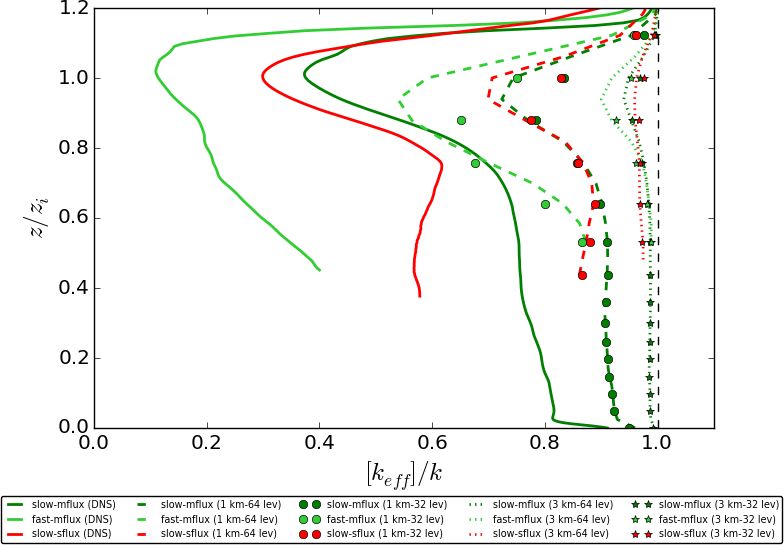
486 C. W. Y. Li et al.: Error induced by neglecting subgrid chemical segregation due to inefficient turbulent mixing
The surface buoyancy flux is set to be Fb (see Appendix A). veloped and statistical equilibrium is attained. The boundary
The parameters ν and κ are the kinematic viscosity and the layer height zi is identified as the height where the buoy-
molecular diffusivity, respectively. k is the unit vector in the ancy variance [b0 b0 ] is maximum away from the surface layer
z direction. The system is statistically homogeneous in the (Garcia and Mellado, 2014). At the end of our simulations,
horizontal direction, such that its statistics depend on z and t the boundary layer height is around 2.2 km. As the boundary
only. layer grows in depth, the corresponding convective velocity
A no-penetration, no-slip boundary condition is imposed and timescales evolve in time. In this study, the convective
at the surface, and a no-penetration, free-slip boundary con- timescale is adopted as the turbulent timescale tturb , which is
dition is imposed at the top boundary. Neumann boundary related to the convective velocity wc by
conditions are imposed for the buoyancy and velocity fields
2
at both the top and the surface to maintain constant fluxes. zi zi 3
The velocity and buoyancy fields are relaxed towards zero tturb = = (1)
wc Fb
and N 2 z, respectively, at the top of the computational do-
main. The height of the top boundary is adjusted so that the (Deardorff, 1970). This turbulent timescale will be used to
turbulent region is far enough from the top to avoid signif- calculate the Damköhler number Da in later sections.
icant interaction. Periodic boundary conditions are imple-
mented in lateral directions. 2.2 Chemical settings
The size of the computational grid is 720 × 720 × 512 for
all simulations (the number of vertical layers is 512). Stretch- 2.2.1 Homogeneous emissions
ing is applied vertically to increase the resolution near the
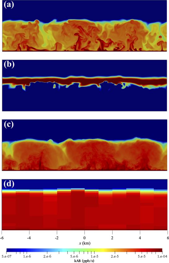
surface in order to resolve the surface layer and to stretch An archetypical entrainment-emission configuration, as typ-
the grid size in the upper portion of the domain end to fur- ically used by past LES studies such as Krol et al. (2000) and
ther separate the top boundary from the turbulent region. Vinuesa and Vilà-Guerau de Arellano (2005), is adopted in
The total simulation domain size is 120L0 ×120L0 ×34.4L0 , our DNS model (see left panel of Fig. 1). The simulations
where L0 is the reference length scale. Together with the ref- are conducted with two theoretical tracers (A and B). Tracer
erence time and velocity timescales T0 and U0 , L0 is used A is emitted from the surface at a constant flux FA at a range
to non-dimensionalise the Navier–Stokes equations (see Ap- of values. Tracer B is entrained from the free troposphere,
pendix A). With typical atmospheric parameters of L0 ∼ in which the mixing ratio of tracer B (hBi0 ) is constantly
100 m and U0 ∼ 1 m s−1 , the horizontal resolution of the and homogeneously fixed at 2 ppb. Tracer C is formed in a
model in use is equivalent to 15 m×15 m with a total domain second-order chemical reaction between tracers A and B:
size of 12 km × 12 km. The resolution is considerably higher
k : A + B → C, (R1)
than those adopted in the previous LES studies, and it is fine
enough to resolve convective turbulent motion in the convec-
where k is the imposed chemical reaction rate. The mixing
tive boundary layer. In the vertical direction, the grid spacing
ratios of the three species, denoted as A, B and C, respec-
increases from 1z = 6.72 m at the surface to 1z = 266.28 m
tively, vary with time with rates equal to
at the top of the domain at 16 km. The vertical grid spacing
vs. height in the first 5 km is shown in Fig. 7 (black line). dC dA dB
We use a sixth-order compact scheme to calculate the spa- =− =− = kAB. (2)
dt dt dt
tial derivatives and a fourth-order Runge–Kutta scheme to
advance the equations in time. The pressure Poisson equa- Neumann boundary conditions are imposed at the boundaries
tion is solved by applying a Fourier decomposition along the of the computational domain on the mixing ratios of the trac-
horizontal directions and solving the resultant set of finite- ers so that the surface flux of tracer A is constant at FA , and
difference equations in the vertical direction to machine ac- the surface fluxes of B and C are zero. In the free troposphere,
curacy (Mellado and Ansorge, 2012). The sensitivity to grid the initial mixing ratios of A and C are zero. The initial mix-
resolution has been tested up to the triple-velocity correlation ing ratio of tracer B is decreased linearly down the boundary
in the transport term of the evolution equation for the turbu- layer to zero on the surface.
lence kinetic energy, observing an error of less than 5 % at the Four emission fluxes of tracer A (FA ), at 0.05, 0.25, 0.5
surface when doubling the spatial resolution. Further details and 1.41 ppb m s−1 , are adopted to test the effect of strong
of the numerical algorithm and the grid-sensitivity studies emissions in an urban environment. The runs are named
can be found in Mellado (2010, 2012), Garcia and Mellado VV05 (from its similar initial conditions as Vinuesa and Vilà-
(2014), and Mellado et al. (2017). Guerau de Arellano, 2005), mflux, sflux and ssflux, respec-
The simulations are terminated after a total simulation tively. As a reference, in the ssflux run, the characteristic
time equivalent to 4.5 h, during which the boundary layer mixing ratio scale for tracer A (hAi0 ) is equal to that of
grows convectively. The simulation time represents the hours tracer B (hBi0 ). These characteristic scales are used in the
from sunrise to midday, when the boundary layer is well de- non-dimensionalisation of Eq. (2) (see Appendix A). Two
Atmos. Chem. Phys., 21, 483–503, 2021 https://doi.org/10.5194/acp-21-483-2021C. W. Y. Li et al.: Error induced by neglecting subgrid chemical segregation due to inefficient turbulent mixing 487
Figure 1. Schematic diagrams of the configurations of the DNS runs with homogeneous emissions (a) and heterogeneous emissions (b).
Table 1. The names and simulation parameters of the DNS runs, including (a) the imposed chemical reaction rate k and the surface emission
flux of tracer A, FA , for the simulations with homogeneous emissions and (b) plus the length of heterogeneity (dx) for the simulations with
heterogeneous emissions.
(a) Homogeneous emissions
Case k (ppb−1 s−1 ) FA (ppb m s−1 )
Slow-VV05 4.75 × 10⁻⁴ 0.05
Fast-VV05 4.75 × 10⁻³ 0.05
Slow-mflux 4.75 × 10⁻⁴ 0.25
Fast-mflux 4.75 × 10⁻³ 0.25
Slow-sflux 4.75 × 10⁻⁴ 0.50
Fast-sflux 4.75 × 10⁻³ 0.50
Slow-ssflux 4.75 × 10⁻⁴ 1.41
Fast-ssflux 4.75 × 10⁻³ 1.41
(b) Heterogeneous emissions
Case dx (km) k (ppb−1 s−1 ) FA (ppb m s−1 )
dx = 1 km
Slow-1 km-VV05 1 4.75 × 10⁻⁴ 0.05
Fast-1 km-VV05 1 4.75 × 10⁻³ 0.05
Slow-1 km-sflux 1 4.75 × 10⁻⁴ 0.5
Fast-1 km-sflux 1 4.75 × 10⁻³ 0.5
dx = 2 km
Slow-2 km-VV05 2 4.75 × 10⁻⁴ 0.05
Fast-2 km-VV05 2 4.75 × 10⁻³ 0.05
Slow-2 km-sflux 2 4.75 × 10⁻⁴ 0.5
Fast-2 km-sflux 2 4.75 × 10⁻³ 0.5
dx = 6 km
Slow-6 km-VV05 6 4.75 × 10⁻⁴ 0.05
Fast-6 km-VV05 6 4.75 × 10⁻³ 0.05
Slow-6 km-sflux 6 4.75 × 10⁻⁴ 0.5
Fast-6 km-sflux 6 4.75 × 10⁻³ 0.5
chemistry cases, namely slow and fast chemistry, are con- reaction rate between isoprene and OH is 0.1 ppb−1 s−1 (Karl
sidered for each of the imposed emission fluxes, with respec- et al., 2004), giving an example illustrating the cases with fast
tive chemical reaction rates of 4.75 × 10⁻⁴ and 4.75 × 10⁻³ chemistry. The names and simulation parameters of the eight
ppb−1 s−1 . In the real atmosphere, the rate of chemical re- simulations are listed in Table 1.
action between NO and O3 is 4.75 × 10⁻⁴ ppb−1 s−1 , cor-
responding to the cases with slow chemistry. Meanwhile, the
https://doi.org/10.5194/acp-21-483-2021 Atmos. Chem. Phys., 21, 483–503, 2021488 C. W. Y. Li et al.: Error induced by neglecting subgrid chemical segregation due to inefficient turbulent mixing
2.2.2 Heterogeneous emissions Similarly the Damköhler number of tracer B can be written
as
For the simulations with heterogeneous emissions, tracers A !1
and B are emitted alternately from patches on the surface z2 3
with widths of 1, 2 and 6 km. The widths of these emission DaB = khAi i . (4)
Fb
patches are referred to in this study as the length of hetero-
geneity dx, similarly as in Ouwersloot et al. (2011).1 The The Damköhler numbers of tracers A and B at the start
A–B–C chemical system (A + B → C) is implemented with (DaA,i and DaB,i ) and at the end (DaA,f and DaB,f ) of each
slow and fast chemistry, as described in Sect. 2.2.1. Both of our simulations are listed in Table 2. For a slow chemical
tracers A and B are emitted at the same imposed flux, with reaction of two initially segregated reactants with the respec-
the two values of emission fluxes at 0.05 ppb m s−1 (VV05) tive Da
1, the chemical lifetime of the reactants is long
and 0.5 ppb m s−1 (sflux) adopted.2 The right panel of Fig. 1 enough for turbulence to mix them in the boundary layer at
shows a schematic diagram describing the simulation config- a rate fast enough that they are homogeneously distributed in
uration. The names and simulation parameters of the twelves a confined volume (e.g. a model grid) in a short time com-
simulations are listed in Table 1. The simulations with het- pared to the chemical lifetime. In that case chemical reac-
erogeneous emissions are run for 8 h, representing the hours tion can occur everywhere in that confined volume and the
from sunrise to the afternoon. These simulations are run for a corresponding volumetric-mean production rate of tracer C
longer time than those with homogeneous emissions because can be approximated as the product of k and the volumet-
the statistical equilibrium takes a longer time to be attained ric means of the reactants (khAihBi). On the other hand, for
with heterogeneous emissions. fast reactions with the respective Da > 1, the reactants are
In the context of an urban environment, the second-order not well mixed by turbulence during the theoretical chem-
chemical reaction imposed in our simulations can be consid- ical lifetime of the reactants, such that they can react only
ered analogous to the reaction between NO and peroxyl rad- in a fraction of the confined volume where turbulent motion
ical derivatives (RO2 ) from the oxidation of VOCs, which brings the two species together. In that case the volumetric-
is the limiting reaction of ozone production in the VOC- mean of the production rate of tracer C also depends on the
limited regime. The VOCs are often emitted from sources turbulent timescale and would be overestimated by khAihBi.
segregated from NO at very high fluxes in urban areas. The Hence, the Damköhler number can indicate whether the ef-
involved chemical reactions are often relatively fast. For in- fect of turbulent mixing on a chemical reaction is signifi-
stance, the reaction rate between NO and acetone peroxy cant in the flow. For instance, the eddy turnover timescale for
radical (CH3 COCH2 O2 ), which is a common VOC species large-scale eddies in a CBL is typically 102 –103 s, to which
found in urban environments (Brasseur and Jacob, 2017; Li, the chemical lifetime of NOX and O3 in the boundary layer
2019), is 0.503 ppb−1 s−1 (Manion et al., 2008), giving an is comparable (102 –105 ). Therefore, the turbulent motions in
example for the fast-chemistry cases in our simulations with the CBL potentially affect any chemical reaction occurring at
heterogeneous emissions. a rate higher than that between NO and O3 .
To quantify the chemistry–turbulence interaction at the
2.3 Quantifying the chemistry–turbulence interaction molecular diffusion spatio-temporal scale, the Kolmogorov
Damköhler numbers are also calculated in some of simula-
Two numbers are mainly employed to quantify the effect of tions. The definition of Kolmogorov Damköhler number is
turbulent mixing on chemical reaction, namely the Damköh- adopted from Vilà-Guerau de Arellano et al. (2004), i.e.
ler number Da and the effective chemical reaction rate keff .
The first number, the Damköhler number (Da), is defined as tk
Dak,A =
the ratio between the turbulent timescale (tturb ) and the chem- tchem,A
ical timescales (tchem ) (Damköhler, 1940). For a second-
for tracer A and similarly for tracer B (Dak,B ) by replacing
order chemical reaction A + B → C, the Damköhler number
the denominator with tchem,B . The Kolmogorov timescale tk
of tracer A is given by
is around 10 s for all the simulations (Garcia and Mellado,
!1 2014).
tturb zi /wc z2 3
The second number, the effective chemical reaction rate
DaA = = = khBi i . (3) (keff ), can quantitatively measure the actual chemical reac-
tchem,A 1/khBi Fb
tion rate averaged in a confined volume under the consid-
eration of chemical segregation due to inefficient turbulent
1 Note that the length of heterogeneity referred to in this study is
mixing (Vinuesa and Vilà-Guerau de Arellano, 2005), and it
equivalent to half of the length denoted in Ouwersloot et al. (2011). can be written as
2 Note that the adopted emission fluxes are doubled from the val-
hA0 B 0 i
ues in the simulations with homogeneous emissions in order to con-
serve the total fluxes. keff = 1 + k, (5)
hAihBi
Atmos. Chem. Phys., 21, 483–503, 2021 https://doi.org/10.5194/acp-21-483-2021C. W. Y. Li et al.: Error induced by neglecting subgrid chemical segregation due to inefficient turbulent mixing 489
Table 2. The initial Damköhler numbers DaA,i and DaB,i , and final Damköhler numbers DaA,f and DaB,f with the resultant normalised
effective chemical reaction rate keff /k in the DNS runs with (a) homogeneous emissions and (b) heterogeneous emissions.
Case DaA,i DaB,i DaA,f DaB,f keff /k
(a) Homogeneous emissions
Slow-VV05 0.1438 0.0094 0.6051 0.0405 0.9652
Fast-VV05 1.4377 0.0938 5.7148 0.0688 0.8687
Slow-mflux 0.1531 0.0291 0.0143 12.7801 0.2350
Fast-mflux 1.5306 0.2907 0.0472 127.6096 0.0455
Slow-sflux 0.1531 0.0214 0.0028 29.8211 0.1225
Fast-sflux 1.5306 0.2142 0.0033 298.1865 0.0304
Slow-ssflux 0.1531 0.0560 0.0002 99.7068 0.0819
Fast-ssflux 1.5306 0.5602 4.8058 × 10⁻⁵ 997.0659 0.0226
(b) Heterogeneous emissions
dx = 1 km
Slow-1 km-VV05 0.0029 0.0029 0.1347 0.1347 1.0184
Fast-1 km-VV05 0.0290 0.0289 0.4896 0.4894 0.9094
Slow-1 km-sflux 0.0070 0.0070 1.3364 1.3392 0.5053
Fast-1 km-sflux 0.0740 0.0740 8.9180 8.9452 0.1365
dx = 2 km
Slow-2 km-VV05 0.0024 0.0024 0.1442 0.1453 0.9952
Fast-2 km-VV05 0.0241 0.0241 0.5656 0.5766 0.7634
Slow-2 km-sflux 0.0069 0.0069 1.9957 2.0217 0.3068
Fast-2 km-sflux 0.0686 0.0686 16.1687 16.4241 0.0487
dx = 6 km
Slow-6 km-VV05 0.0036 0.0036 0.2017 0.2034 0.6650
Fast-6 km-VV05 0.0357 0.0357 1.3034 1.3213 0.2068
Slow-6 km-sflux 0.0110 0.0110 7.0356 7.1541 0.0312
Fast-6 km-sflux 0.1070 0.1070 67.8306 69.0153 0.0034
where the angle-bracketed and primed terms are the means are correlated, then IS > 1. With the DNS model fully re-
and the deviations from the means, respectively, of the solving the chemical segregation in the boundary layer, the
Reynolds-decomposed concentrations. error from a complete-mixing or coarse-grid model can be
The error induced by neglecting such chemical segregation calculated by
in a complete-mixing model, in which both tracers A and B
E = keff, cm − keff, DNS , (8)
are assumed to be evenly distributed throughout the boundary
layer, can be written as where keff, cm is the calculated boundary-layer-averaged ef-
fective chemical reaction rate in a complete-mixing or
keff coarse-grid model, and keff, DNS is the calculated value in the
E = 1− = −IS , (6)
k corresponding DNS model.
When one considers a confined volume within a horizon-
where the segregation coefficient
tal layer at a specific height z, the corresponding effective
hA0 B 0 i chemical reaction rate also varies with height. The height-
IS = (7) dependent effective chemical reaction rate can be written as
hAihBi
a function of z:
0 0 !
represents the state of mixing of tracers A and B in the AB
boundary layer (e.g. Danckwerts, 1952; Vinuesa and Vilà- [keff ] (z) = 1 + k = (1 + [IS ] (z))k. (9)
[A] [B]
Guerau de Arellano, 2003). If tracers A and B are completely
mixed, then IS = 0. If tracers A and B are completely segre- The square-bracketed terms denote the horizontal means of
gated, then IS = −1. If tracers A and B are emitted simulta- the quantities. The corresponding height-dependent error in-
neously and at the same location so that their concentrations duced by neglecting chemical segregation by a model that
https://doi.org/10.5194/acp-21-483-2021 Atmos. Chem. Phys., 21, 483–503, 2021490 C. W. Y. Li et al.: Error induced by neglecting subgrid chemical segregation due to inefficient turbulent mixing
assumes tracers A and B are well-mixed horizontally within rates are also similar to the values of 96 % and 85 % reported
a horizontal layer at z is then in Vinuesa and Vilà-Guerau de Arellano (2005). Therefore,
our DNS model gives similar boundary-layer-averaged val-
[keff ] (z) ues of keff as the LES model adopted in Vinuesa and Vilà-
[E](z) = 1 − = − [IS ] (z), (10)
k Guerau de Arellano (2005). When comparing our vertical
where the height-dependent segregation coefficient is profiles of the horizontally averaged effective chemical reac-
tion rate (Fig. 4) with the vertical profiles of the segregation
0 0
AB coefficient presented in Vinuesa and Vilà-Guerau de Arel-
[IS ] (z) = . (11) lano (2005), the profiles of the two studies in general share
[A] [B]
similar shapes, with the largest magnitude of segregation all
occurring just below the top of the boundary layer. For in-
3 Results of the DNS runs stance, the maximum values of [keff ] are 83 % and 62 % of k
in our slow-VV05 and fast-VV05 runs, respectively.3 How-
3.1 Homogeneous emissions ever, our profiles show more prominent minima near the top
of the surface layer, which shows the effect of the higher ver-
3.1.1 Reference cases with rural emission flux
tical resolution in the DNS model.
For both VV05 runs, all the tracers are relatively well mixed
3.1.3 The effect of strong emission fluxes
in the mixed layer. Tracer A is largely consumed in the mixed
layer, while tracer B is in excess so that its concentration re- When the emission fluxes of tracer A increase to urban val-
mains essentially constant. The reaction between tracers A ues beyond 0.25 ppb m s−1 in the mflux, sflux and ssflux runs,
and B can then be considered a pseudo first-order reaction, tracer A accumulates and is in excess in most of the bound-
and the corresponding production term kAB ≈ k 0 A (plotted ary layer. On the other hand, tracer B is almost completely
in the top panel of Fig. 2) is dependent only on the concentra- depleted in the lower part of the boundary layer. As the emis-
tion of tracer A, where k 0 = kB is the pseudo first-order rate sion flux of tracer A increases and/or the chemistry becomes
coefficient (Hobbs, 2000; Jacobson and Jacobson, 2005). In faster, the chemical timescale of tracer B shortens, so the
this situation, tracer A is said to be the limiting reactant, and depth where tracer B can be replenished from the free tro-
the chemical reaction between tracers A and B is tracer-A posphere becomes narrower. Tracer C is mostly produced
limiting (Zumdahl, 1992). As the production of tracer C is near the top of the boundary layer, as indicated in the colour
also tracer-A limiting, the vertical fluxes of tracer C (the ma- map of the production term in the middle panel of Fig. 2.
genta lines in Fig. 3) in these two cases are both positive, sim- The chemical system now transits to the so-called “diffusion-
ilar to those of tracer A (not shown), indicating that tracers A limited” reaction (Sykes et al., 1994), where the reaction be-
and C are both correlated with the updraught. As the chem- tween tracers A and B depends on the availability of tracer B
istry shifts from slow to fast, the height with the maximum and hence is tracer-B limiting.
flux of tracer C transits from near the top of the boundary The shift of the reaction from tracer-A limiting to tracer-
layer to near the surface. This is due to the increasing life- B limiting can also be seen from the profiles of the vertical
time of tracer B with an increasing chemical reaction rate. fluxes of tracer C in Fig. 3 (sflux in red and ssflux in cyan).
As more tracer A is consumed, more tracer B can flow down The fluxes of tracer C now become negative, indicating that
the boundary layer without being consumed; hence, more tracer C is downdraught correlated, as is tracer B. As the
tracer C is produced at a lower altitude in the boundary layer emission flux of tracer A increases, the maximum of the pro-
where tracer A is available. As indicated by a large Damköh- duction term shifts from the top of the surface layer to near
ler number of tracer A (DaA,f = 5.71 > 1), the mixing be- the top of the boundary layer closer to the source of tracer
tween tracers A and B hence becomes less efficient, resulting B. These cases are also characterised by very large values of
in a larger segregation between the two tracers. DaB,f instead of a large DaA,f as in the fast-VV05 run (see
Table 2). Since the chemical transformation of the reactant
3.1.2 Comparison with previous LES studies
that is relatively less abundant than the other reactant is in-
We use the results of the two VV05 runs to compare with fluenced more by turbulent mixing (Vilà-Guerau de Arellano
those presented in the LES study of Vinuesa and Vilà- et al., 2004), DaB,f is now a better indicator for the role of
Guerau de Arellano (2005). The horizontal and vertical res- 3 Unfortunately we cannot compare the vertical profiles of our
olutions of their LES model are 50 and 25 m, respectively, horizontally averaged effective chemical reaction rate with the ver-
roughly 4 times coarser than the resolutions of our DNS tical profiles of the segregation coefficient presented in Vinuesa and
model. From our DNS model, the resultant boundary-layer- Vilà-Guerau de Arellano (2005) quantitatively, as the latter profiles
averaged effective chemical reaction rates keff are 96.5 % and are from the LES studies in Vinuesa and Vilà-Guerau de Arellano
86.9 % of the imposed rate k for our slow-VV05 and fast- (2003), which adopted a different set of initial conditions as Vinuesa
VV05 runs, respectively (see last column of Table 2). These and Vilà-Guerau de Arellano (2005) and our study.
Atmos. Chem. Phys., 21, 483–503, 2021 https://doi.org/10.5194/acp-21-483-2021C. W. Y. Li et al.: Error induced by neglecting subgrid chemical segregation due to inefficient turbulent mixing 491 Figure 2. Colour maps of the distribution of the production term (kAB) at the end of the simulations with homogeneous emissions for (a) the cases slow-VV05 and (b) slow-mflux. (c) Same colour map for the same case as in (a) but with time averaged for the last 30 min of the simulation. (d) Same colour map for the same case as in panel (a) but in the 1 km-64 lev coarse-grid model. turbulent mixing on chemical reactions than DaA,f . Sum- The errors induced by neglecting the subgrid chemical seg- marising the simulations with homogeneous emissions, one regation become significant when Dak,lim reaches the order can observe from Fig. 8 (black circles) that the deviation of of around 10−1 . keff from the imposed rate k (or the error from the complete- For the runs with urban emission fluxes, the boundary- mixing model) increases with the increased Damköhler num- layer-averaged effective chemical reaction rate keff is very ber of the limiting reactant (Dalim ), where Dalim = DaA,f low even with slow chemistry. With slow chemistry, keff is when the reaction is tracer-A limiting and Dalim = DaB,f only 23.5 %, 12.3 % and 8.2 % of the imposed rate k in the when the reaction is tracer-B limiting. This transition occurs mflux, sflux and ssflux runs, respectively. With fast chem- when Dalim reaches the order of 10. A similar concept can istry, keff further drops to 4.6 %, 3.0 % and 2.3 % of k, re- also be applied to the corresponding Kolmogorov Damköhler spectively. These low values of keff imply that if the surface number, where the limiting Kolmogorov Damköhler number emission of a pollutant is so strong that the reaction is lim- (Dak,lim ) is introduced (refer to the upper x axis of Fig. 8). ited by the availability of the entrained reactant, the resultant https://doi.org/10.5194/acp-21-483-2021 Atmos. Chem. Phys., 21, 483–503, 2021
492 C. W. Y. Li et al.: Error induced by neglecting subgrid chemical segregation due to inefficient turbulent mixing
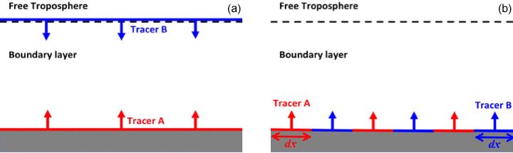
Figure 5. Vertical profiles of the horizontally averaged normalised
Figure 3. Vertical profiles of the horizontally averaged vertical flux effective chemical reaction rate [keff ]/k (and the horizontally aver-
of tracer C [C 0 w 0 ] with homogeneous emissions for varied cases aged segregation coefficient [IS ] (upper x axis)) with heterogeneous
time averaged for the last 30 min of the simulations. emissions for varied cases time averaged for the last 30 min of the
simulations.
3.2 Heterogeneous emissions
With the emissions of tracers A and B heterogeneously dis-
tributed on the surface, the segregation is maximum at the
surface with its magnitude decreasing with increasing alti-
tude, as seen from the vertical profiles of the horizontally
averaged segregation coefficient ([IS ](z)) in Fig. 5. It is be-
cause under this setting mixing is most difficult near the sur-
face where the tracers are emitted separately. This descrip-
tion of the profiles agrees with the results of the simula-
tions with heterogeneous emissions presented in Krol et al.
(2000) and Vinuesa and Vilà-Guerau de Arellano (2005), de-
spite that they implemented a different emission configura-
tion with a Gaussian function imposed on the surface emis-
sion flux. To examine how the segregation between tracers A
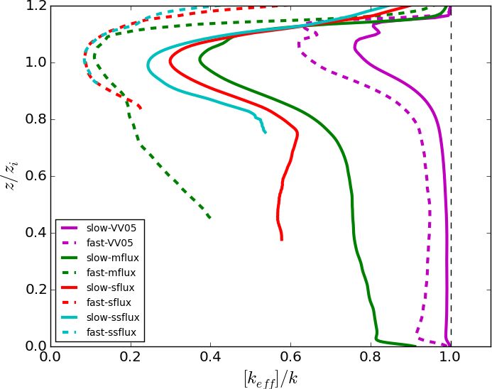
Figure 4. Vertical profiles of the horizontally averaged normalised and B changes with the emission flux and the imposed chem-
effective chemical reaction rate [keff ]/k with homogeneous emis-
ical reaction rate, the results of the set of simulations with the
sions for varied cases time averaged for the last 30 min of the sim-
ulations. Note that the vertical profiles are not plotted at altitudes
length of heterogeneity (dx) of 2 km (all plotted in red) are
where the concentration of tracer B is equal to zero. first compared. In the slow-2 km-VV05 run (dashed red line),
the magnitude of [IS ] decreases with increasing altitude in
the boundary layer, so at a height above 0.8zi , [IS ] becomes
overestimation of the actual chemical reaction from an as- larger than zero, meaning that tracers A and B are not only
sumption of complete mixing can be substantial (in our cases well mixed but also that their flows are correlated. This re-
up to 98 %) for any reaction with reaction rate equivalent to sults in [keff ] > k, where the assumption of complete mixing
or faster than that between NO and O3 . The vertical profiles in the model grid will underestimate the reaction rate. This
of the horizontally averaged effective chemical reaction rate phenomenon is also reported in Ouwersloot et al. (2011),
in Fig. 4 show that the maximum segregation between trac- showing [IS ] > 0 at higher altitudes in their LES simulations
ers A and B still occurs near the top of the boundary layer. with heterogeneous isoprene emission fluxes. On the other
With fast chemistry, the effective chemical reaction rate at hand, as the surface emission flux increases to 0.5 ppb m s−1
that altitude can even drop to around 10 % of the imposed in the slow-2 km-sflux run (red solid line), [IS ] > 0 only at
rate. the height above 0.98zi .
When shifting from slow to fast chemistry (dotted red
line), the magnitude of the segregation further increases, re-
Atmos. Chem. Phys., 21, 483–503, 2021 https://doi.org/10.5194/acp-21-483-2021C. W. Y. Li et al.: Error induced by neglecting subgrid chemical segregation due to inefficient turbulent mixing 493
sulting in a boundary-layer-averaged value of −0.95. The
segregation at the top of the boundary layer remains high,
with [IS ] = −0.8. Sometimes the segregation caused by an
increase in imposed reaction rate k can reduce keff so much
that merely increasing k can no longer increase the produc-
tion of tracer C. This happens between the two 6 km-sflux
runs (check Table 2 for their resultant keff ). When shifting
from slow chemistry to fast chemistry, keff drops 9.18 times,
such that it in turn cancels the effect of the 10 times increase
in k. This results in similar amounts of tracer C produced
in the two 6 km-sflux runs, with the mixing ratio of tracer C
equal to 1.58 and 1.60 ppm at the end of the simulations for
the slow- and fast-chemistry cases, respectively.
To discuss the effect of the length of heterogeneity (dx)
on segregation, the three solid lines in the left panel of Fig. 5,
which indicate the slow-sflux runs at different dx (dx = 1 km
plotted in blue, dx = 2 km in red and dx = 6 km in green),
are compared. In general, the segregation increases with in- Figure 6. Fitted curves of the normalised boundary-layer-averaged
creasing dx. This agrees with the conclusion from Ouwer- effective chemical reaction rate keff /k against the final Damköh-
sloot et al. (2011). For the cases with dx = 1 km and dx = ler numbers Daf for the simulations with heterogeneous emissions
2 km, one can still observe a decrease in the magnitude of the with different lengths of heterogeneity (dx). afit refers to the fitted
segregation with increasing altitude, with the corresponding slope for the square law between log(keff /k) and log(Daf ) corre-
sponding to different dx values.
boundary-layer-averaged IS equal to −0.49 and −0.69, re-
spectively. However, for dx = 6 km, the segregation remains
almost constant throughout the mixed layer and starts to de-
crease only below the top of the boundary layer. This also
results in a very large segregation throughout the boundary
layer, with the boundary-layer-averaged IS equal to −0.97.
This shows a similar phenomenon, as described in Ouwer-
sloot et al. (2011), that as the length of heterogeneity exceeds
a few boundary layer heights,4 i.e. ∼ 3 km at the end of the
simulations, the boundary layer between the two patches that
emit tracers A and B, respectively, barely mix, and the sys-
tem behaves like two individual boundary layers.
Similar to the cases with homogeneous emissions, the in-
creased segregation with increasing surface emission flux
and imposed chemical reaction rate can be indicated by the
relatively large values of the final Damköhler numbers. Since
the boundary-layer-averaged Damköhler numbers of tracers
A and B are statistically the same in the simulations with
heterogeneous emissions, here we take the mean of the two Figure 7. Plot of the vertical grid spacing (dz) (in equivalent to
vertical resolution) vs. height (z) in the DNS model (black), the
numbers to get the averaged final Damköhler number Daf
64 lev coarse-grid models (red) and the 32 lev coarse-grid models
(equal to 1/2(DaA,f + DaB,f )). We then fit Daf with the (blue) in the first 5 km.
normalised boundary-layer-averaged keff /k for the simula-
tions with each dx (check Table 2 for the values). The results
are plotted in Fig. 6. In general, log(keff /k) follows a square −1). As dx increases, afit also increases (see the values in
law with log(Daf ), i.e. log(keff /k) = −afit (log Daf + 1)2 , Fig. 6). However, their relation is unlikely to be linear.
where afit is the fitting coefficient varying with dx. Or in an-
other way, keff /k follows a Gaussian function of Daf , i.e.
keff /k = exp(−afit (log Daf + 1)2 ). The x intercept is cho- 4 Estimating errors from regional models
sen to be −1 because keff ≈ k when Daf .0.1 (or log Daf ∼
In the previous sections, the boundary-layer-averaged effec-
4 Converting the conclusions of Ouwersloot et al. (2011) to our tive chemical reaction rate is compared with the imposed
denotation, the separation of the boundary layer above the different rate in a complete-mixing model that assumes the tracers
emission patches occurs when dx > 8zi . to be completely well mixed in the whole boundary layer.
https://doi.org/10.5194/acp-21-483-2021 Atmos. Chem. Phys., 21, 483–503, 2021494 C. W. Y. Li et al.: Error induced by neglecting subgrid chemical segregation due to inefficient turbulent mixing
However, the horizontal resolutions in regional chemical- of the limiting reactant (Dalim ; see the values in Table 2).
transport models are comparatively high (of the order of One can see that in all runs the errors from all coarse-grid
a few kilometres) with multiple vertical levels within the models are reduced in comparison to the complete-mixing
boundary layer. Such models are often employed when mod- model. The model errors from the coarse-grid models are
elling urban areas. To evaluate the importance of the subgrid largely reduced when Dalim > 10, which corresponds to the
chemistry–turbulence interaction in these regional chemical- simulations with urban surface emission fluxes (mflux, sflux
transport models, we degrade our DNS model to coarse-grid and ssflux). In those runs, the model errors drop from 77 %–
models with two horizontal resolutions (1 and 3 km, with 98 % in the complete-mixing model to 36 %–69 % in the 32-
12 and 4 nodes in the horizontal direction, respectively) and level models and further to 15 %–51 % in the 64-level mod-
two vertical resolutions (labelled 32 and 64 lev, with 32 and els. However, this also means that even with the highest res-
64 nodes in the vertical direction in the whole domain, and olution the model errors are still noticeably significant. Also,
with 10 and 20 levels within the boundary layer, respec- for five out of seven runs (the slow-VV05 run is excluded
tively, when the boundary layer is fully grown), resulting here due to the insignificant errors), a larger reduction of the
in four coarse-grid models, named 1 km-64 lev, 1 km-32 lev, model error is observed with an increased vertical resolution
3 km-64 lev and 3 km-32 lev. Figure 7 shows the respective (from blue + to blue ×) than with an increased horizontal
vertical resolutions of the DNS model and the 64- and 32- resolution (from blue + to red +). The reason behind this is
level coarse-grid models vs. height. These resolutions are se- that tracers A and B are segregated along the vertical direc-
lected according to common grid sizes in regional chemical- tion.
transport models (e.g. Bouarar et al., 2017; Marécal et al., Figure 9 shows the vertical profiles of the horizontally av-
2015). eraged error ([E](z); see Eq. 10) of the four coarse-grid mod-
The tracer concentration fields obtained from the DNS els for the slow-mflux and slow-sflux runs. All coarse-grid
runs are interpolated from the high-resolution DNS model models fail to show the local minimum at the top of the sur-
grids to the lower-resolution coarse-grid model grids. The face layer, as the surface layer is too thin for these models
volumetric averages of tracer concentrations in each model to resolve. They also show a less prominent minimum at the
grid are then calculated. The statistics of these resolution- top of the boundary layer. The distinct underestimation of
degraded concentration fields are then calculated as in [E] in the surface layer and entrainment zone indicates that
Sect. 3. The chemical production terms from a coarse-grid high vertical resolution is especially important to resolve the
model and the corresponding DNS run are plotted in the top chemical segregation around these two zones.
and bottom panels of Fig. 2, respectively, to illustrate the ef-
fect of resolution degrading. In contrast to the DNS model, 4.2 Heterogeneous emissions
the coarse-grid model can no longer resolve the chemical
segregation within each of its model grids. The boundary- The errors from the four coarse-grid models (E) in the simu-
layer-averaged normalised effective chemical reaction rates lations with heterogeneous emissions are then plotted against
keff /k of the four coarse-grid models averaged over the last the errors from the corresponding complete-mixing model
1.5 h of the corresponding simulations are subtracted from (Ecm ) in Fig. 10. These data points are categorised with dif-
the values of keff /k from our DNS model (last column of Ta- ferent lengths of heterogeneity (dx) implemented in the cor-
ble 2) to obtain the boundary-layer-averaged errors from the responding simulations. The dashed line indicates the value
coarse-grid models induced by neglecting the subgrid chem- where E = Ecm . The points below the dashed line show the
ical segregation (E) (see Eq. 8). These errors are listed in cases for which the corresponding coarse-grid model im-
Table 3. The second column is the error from a complete- proves from the complete-mixing model, while those above
mixing model (Ecm ), calculated from Eq. (6). Note that the the dashed line show a deterioration. Contrary to the simula-
errors are listed in percentages. Positive values indicate over- tions with homogeneous emissions the coarse-grid models do
estimation of the model from the actual chemical reaction not always perform better than the complete-mixing model,
rate, and negative values indicate underestimation. The dom- especially when the horizontal model grid size is larger than
inance of positive values shows that the coarse-grid models, the length of heterogeneity. It is because under this condi-
similar to the complete-mixing model, usually overestimate tion, the model grid fails to resolve the heterogeneity of the
the actual chemical reaction rate. emission sources. This also applies to the simulations with
dx = 1 km in the 1 km resolution coarse-grid models, as the
4.1 Homogeneous emissions model grids are slightly offset from the emission patches. In
these runs, the coarse-grid models mix the originally segre-
We take a closer look at the results of the simulations with gated tracers in the lower layers at a higher concentration
homogeneous emissions as described in Sect. 3.1. Figure 8 than the complete-mixing model, in which the latter artifi-
shows the model errors from the complete-mixing model cially mixes the tracers all over the whole boundary layer
(black circles) and the four coarse-grid models (+ and × and dilutes the tracer concentrations. That is why the coarse-
marks) against the corresponding final Damköhler number grid models give larger overestimations. The model with the
Atmos. Chem. Phys., 21, 483–503, 2021 https://doi.org/10.5194/acp-21-483-2021C. W. Y. Li et al.: Error induced by neglecting subgrid chemical segregation due to inefficient turbulent mixing 495 Figure 8. Plot of the model errors E in percentage from the complete-mixing model (black circles) and the four coarse-grid models (+ and × in red and blue) against the corresponding Damköhler number of the limiting reactant (Dalim ) (and the corresponding Kolmogorov Damköhler number of the limiting reactant (Dak,lim ) (upper x axis)) for the simulations with homogeneous emissions. Figure 9. Vertical profiles of the horizontally averaged normalised effective chemical reaction rate [keff ]/k from the four coarse-grid models with homogeneous emissions for the slow-mflux (in dark green), fast-mflux (in light green) and slow-sflux (in red) cases time averaged for the last 30 min of the simulations. Note that the vertical profiles are not plotted at altitudes where the concentration of tracer B is equal to zero. https://doi.org/10.5194/acp-21-483-2021 Atmos. Chem. Phys., 21, 483–503, 2021
496      C. W. Y. Li et al.: Error induced by neglecting subgrid chemical segregation due to inefficient turbulent mixing

                                                                       ment such correction is to substitute the imposed chemical
                                                                       reaction rate k by the effective rate keff which, as shown in
                                                                       Fig. 8, can be expressed as a function of Dalim . The results
                                                                       from the simulations with heterogeneous emissions (Fig. 6)
                                                                       suggest that keff additionally depends on the length of het-
                                                                       erogeneity (dx). When considering increasing model reso-
                                                                       lution to reduce the errors induced by neglecting subgrid
                                                                       chemical segregation, we learn from Sect. 4 that whether it
                                                                       is more effective to increase the horizontal or vertical reso-
                                                                       lution depends on the direction of the initial segregation of
                                                                       the reactant sources. High resolution is in particular neces-
                                                                       sary around the surface layer and entrainment zone. When
                                                                       the reactant sources are horizontally segregated, it is essen-
                                                                       tial that the horizontal resolution of the model is fine enough
                                                                       to resolve the emission heterogeneity. Otherwise, increasing
                                                                       the vertical resolution can induce even larger model errors.
                                                                          There are additional points to note in our estimations.
                                                                       When arriving at our conclusion of the dependency of keff
                                                                       on Dalim , we increase Dalim by shortening the correspond-
Figure 10. Plot of model errors in percentage, categorised with dif-
ferent lengths of heterogeneity (dx), from the four coarse-grid mod-   ing chemical timescale with increased imposed k and emis-
els (E) against the corresponding errors from the complete-mixing      sion fluxes. One should not neglect the dependency of
model (Ecm ) for the simulations with heterogeneous emissions.         Dalim on the buoyancy fluxes, which determine the turbu-
                                                                       lent timescale. However, we expect to see a similar keff de-
                                                                       pendency on Dalim when one repeats the simulations with
higher vertical resolution overestimates the reaction rate even        increasing buoyancy fluxes instead.
more, as its first layers are thinner and hence contain even              By increasing the emission fluxes to urban values in
higher concentrations of the artificially mixed tracers in the         Sect. 3.1.3, it is shown that the effective chemical reaction
lower-level grids.                                                     rate can be much smaller than the values reported in pre-
   For the simulations with dx = 6 km, the coarse-grid mod-            vious studies under rural conditions (e.g. Vinuesa and Vilà-
els always perform better than the complete-mixing model.              Guerau de Arellano, 2003, 2005). However, it should be also
In these simulations, the horizontal grids in the coarse-grid          noted that the chemical segregation is particularly large in
models can always resolve the emission heterogeneity. Note             these simulations, because one of the reactants (in this case
that the reduction of the errors from the coarse-grid models           tracer B) is depleting. Despite the large deviation of keff from
is larger for the increased horizontal than vertical resolution,       k, the production term kAB is anyway small due to the low
as tracers A and B are now segregated in the horizontal di-            concentration of tracer B. Therefore, the actual effect on the
rection.                                                               calculated concentration of tracer B may not be as large as
                                                                       one may expect from the overestimation of keff . A similar
                                                                       reasoning also applies to tracer A. When the emission flux of
5     Discussions                                                      tracer A is large, the main process affecting the concentra-
                                                                       tion of tracer A is emission instead of chemistry. However,
5.1    Implications for regional modelling of urban                    the effect of chemical segregation on the concentrations of
       environments                                                    the product tracer C is still worth noticing.
                                                                          Unlike other studies (e.g. Ouwersloot et al., 2011; Dlugi
Although the DNS runs in this work are only conducted                  et al., 2019; Kim et al., 2016; Li et al., 2016, 2017) in which
in idealised conditions, they can provide insights into and            multiple-reaction chemical systems are employed, our work
estimations of the errors induced by neglecting the sub-               mostly focuses on an idealised second-order chemical reac-
grid chemical segregation due to inefficient turbulent mix-            tion of two non-specific reactive species. This approach al-
ing in larger-scale models. The simulations with homoge-               lows us to interpret our work for any second-order chemi-
neous emissions (Sect. 3.1) show significant errors in the             cal reactions. For a chemical species involved in a multiple-
low-resolution model under strong emission flux conditions,            reaction chemical system, like O3 , one can still calculate the
which are indicated by a large (> 1) Damköhler number of               net impact of chemical segregation by considering the errors
the limiting reactant (Dalim ). This suggests that Dalim > 1           of all reactions in which the species is involved. However,
can be taken as a condition in the model under which the               it is also important to notice that the net impact of chem-
chemical calculation should be corrected by taking the sub-            ical segregation on such a species would in general be re-
grid chemical segregation into account. One way to imple-              duced with the increasing complexity of the chemical sys-

Atmos. Chem. Phys., 21, 483–503, 2021                                                     https://doi.org/10.5194/acp-21-483-2021
You can also read