OpenDrift v1.0: a generic framework for trajectory modelling - GMD
←
→
Page content transcription
If your browser does not render page correctly, please read the page content below
Geosci. Model Dev., 11, 1405–1420, 2018
https://doi.org/10.5194/gmd-11-1405-2018
© Author(s) 2018. This work is distributed under
the Creative Commons Attribution 4.0 License.

OpenDrift v1.0: a generic framework for trajectory modelling
Knut-Frode Dagestad1 , Johannes Röhrs1 , Øyvind Breivik1,3 , and Bjørn Ådlandsvik2
1 Norwegian Meteorological Institute, Bergen, Norway
2 Institute
         of Marine Research, Bergen, Norway
3 Geophysical Institute, University of Bergen, Bergen, Norway

Correspondence: Knut-Frode Dagestad (knutfd@met.no)

Received: 20 August 2017 – Discussion started: 30 August 2017
Revised: 6 February 2018 – Accepted: 19 February 2018 – Published: 13 April 2018

Abstract. OpenDrift is an open-source Python-based frame-        1    Introduction
work for Lagrangian particle modelling under development
at the Norwegian Meteorological Institute with contribu-         Lagrangian trajectory models are used to predict the path-
tions from the wider scientific community. The framework         ways and transformations of various types of objects and sub-
is highly generic and modular, and is designed to be used        stances drifting in the ocean or in the atmosphere. There are
for any type of drift calculations in the ocean or atmo-         many practical and academic applications, including predic-
sphere. A specific module within the OpenDrift framework         tion of
corresponds to a Lagrangian particle model in the traditional
                                                                     – oil drift and weathering to aid mitigation and cleanup
sense. A number of modules have already been developed,
                                                                       operations (Jones et al., 2016);
including an oil drift module, a stochastic search-and-rescue
module, a pelagic egg module, and a basic module for at-             – drifting objects for search and rescue (Breivik and
mospheric drift. The framework allows for the ingestion of             Allen, 2008; Breivik et al., 2011, 2013);
an unspecified number of forcing fields (scalar and vectorial)
from various sources, including Eulerian ocean, atmosphere           – ichthyoplankton transport (fish eggs and larvae) for
and wave models, but also measurements or a priori values              stock assessments (Röhrs et al., 2014); and
for the same variables. A basic backtracking mechanism is
inherent, using sign reversal of the total displacement vector       – microplastics suspended in the ocean (van Sebille et al.,
and negative time stepping. OpenDrift is fast and simple to            2012, 2015).
set up and use on Linux, Mac and Windows environments,
                                                                    Table 1 lists some commonly used trajectory models and
and can be used with minimal or no Python experience. It is
                                                                 their applications. Additionally, many individual researchers
designed for flexibility, and researchers may easily adapt or
                                                                 or research groups have been developing trajectory model
write modules for their specific purpose. OpenDrift is also
                                                                 codes for in-house use, without publishing (or naming) a
designed for performance, and simulations with millions of
                                                                 software code.
particles may be performed on a laptop. Further, OpenDrift
                                                                    Lagrangian tools fall in two broad categories: either the
is designed for robustness and is in daily operational use for
                                                                 trajectories are computed along with the velocity fields as
emergency preparedness modelling (oil drift, search and res-
                                                                 part of the ocean or atmospheric circulation model, e.g. so-
cue, and drifting ships) at the Norwegian Meteorological In-
                                                                 called floats in the regional ocean modelling system (ROMS)
stitute.
                                                                 (Shchepetkin and McWilliams, 2005). This is known as “on-
                                                                 line” trajectory computations and has the advantage that no
                                                                 separate model is needed. Alternatively, the trajectories can
                                                                 be computed “offline” after completion of the Eulerian model
                                                                 simulation(s). This is the approach taken for OpenDrift and
                                                                 is also necessary for a generic framework as the trajectories

Published by Copernicus Publications on behalf of the European Geosciences Union.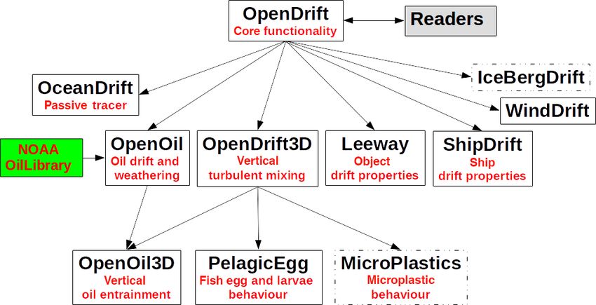
1406                                   K.-F. Dagestad et al.: OpenDrift v1.0: a generic framework for trajectory modelling

depend in many cases on forcing from a range of fields stem-        2     Software design
ming from more than just one Eulerian model. This is, e.g.
the case for oil drift and search-and-rescue models, which          To meet the requirements listed above, a simple and flexi-
both require wind as well as currents (and wave forcing             ble object-oriented data model has been designed, based on
in the case of oil drift) to properly account for the advec-        two main classes. One class (“Reader”) is dedicated to ob-
tion and transformation of the particles. For such emergency        taining forcing data from external sources, as described in
preparedness purposes, offline models are the only option           Sect. 2.1. A generic class for a trajectory model instance
fast enough to meet the requirements of operational agen-           (“BaseModel”) is described in Sect. 2.2. This class contains
cies. Other advantages of offline models are that modifica-         functionality which is common to all drift models, whereas
tions (sensitivity tests) of the drift algorithms may be tested     advection (propagation) and transformation of elements is
quickly without needing to rerun the full Eulerian model, and       left for purpose-specific subclasses.
also that simulations backwards in time may be performed.
   Existing trajectory models are in most cases tied to a spe-      2.1    Reader class
cific application, and may not be applied to other drift appli-
                                                                    The class Reader obtains forcing data (e.g. wind, waves and
cations without compromising quality or flexibility. In many        currents) from any possible source and provides this to any
cases, trajectory models are also tied to a specific Eulerian       OpenDrift model through a common interface. To avoid du-
model, or even a particular institutional ocean model setup,        plication of code, a parent class “BaseReader” contains func-
limiting usability for other institutes or researchers. Often, it   tionality which is common to all Readers, whereas specific
is also required that Eulerian forcing data must be in a spe-       subclasses take care of only the tasks which are specific to
cific file format. This raises the time and effort needed to        a particular source of data, e.g. how to decode and inter-
set up a trajectory model. Further, in an operational setup,        pret a particular file format. Two methods must be imple-
the need to convert large files to another format increases         mented by any Reader subclass: (1) a constructor method
both the complexity and computational costs of the process-         which initialises a Reader object and (2) a method to re-
ing chain, compromising robustness.                                 trieve data for given variables, position and time. The con-
                                                                    structor (__init__ in Python) can take any arguments as im-
   The OpenDrift framework has been designed to perform
                                                                    plemented by the specific Reader class, but it is typical to
all tasks which are common to trajectory models, whether            provide a filename or URL from which data shall be obtained
oceanic or atmospheric. In short, the main task is to obtain        by this Reader. The following Python commands initialise a
forcing data from various sources and to use this information       Reader of type NetCDF_CF_generic to obtain data from a
to move (propagate) the elements in space, while potentially        file “ocean_model_output.nc”.
transforming other element properties, such as evaporation
of oil, or growth of larvae. In addition, common function-          >>> from opendrift.readers import reader_
ality includes mechanisms for configuration of simulations,             netCDF_CF_generic
                                                                    >>> r = reader_netCDF_CF_generic.Reader(
seeding of elements, exporting output to file, and tools to
                                                                        "ocean_model_output.nc")
visualise and analyse the output. Additionally, several de-
sign requirements have been imposed on the development              The initialisation typically includes opening and reading
of OpenDrift: (1) platform independence and ease of instal-         metadata from a given file or URL to check which variables
lation and use; (2) simple and rapid implementation of any          are available, and the coverage in time and space. The ac-
purpose-specific processes, yet flexibility to support unfore-      tual reading of the data is, however, not performed yet, but is
seen needs; (3) forcing data from any type of source sup-           delayed until it is known exactly which subset in space and
ported, including Eulerian ocean, atmosphere or wave mod-           time is actually needed (“lazy reading”). The contents can be
                                                                    inspected by printing the object:
els (typically NetCDF or GRIB files), in situ measurements,
vector data sets (e.g. GSHHS coastlines) or analytical fields       >>> print r
for conceptual studies; (4) the ability run fast, even with a       Projection:
large number of elements; (5) simulations forward and back-           +proj=stere +lat_0=90 +lon_0=70 +lat_ts=60
ward in time; (6) robustness for operational use.                     +units=m +a=6.371e+06 +e=0 +no_defs
   In Sect. 2, we describe the overall design of the code and       Coverage: [m]
the general workflow of performing a simulation. In Sect. 3,          xmin: -2952800.000000
we give examples of three specific modules which are in-              xmax: -2712800.000000
                                                                      step: 800   numx: 301
cluded in the OpenDrift repository: search and rescue, oil
                                                                      ymin: -1384000.000000
drift and atmospheric transport. The test suite and example
                                                                      ymax: -1224000.000000
scripts are described in Sect. 4, and graphical user interfaces       step: 800   numy: 201
(web and desktop) are described in Sect. 5. Section 6 pro-            Corners (lon, lat):
vides discussion and conclusions.                                       ( 2.52, 59.90) ( 4.28, 61.89)
                                                                        ( 5.11, 59.32) ( 7.03, 61.26)
                                                                    Vertical levels [m]:

Geosci. Model Dev., 11, 1405–1420, 2018                                              www.geosci-model-dev.net/11/1405/2018/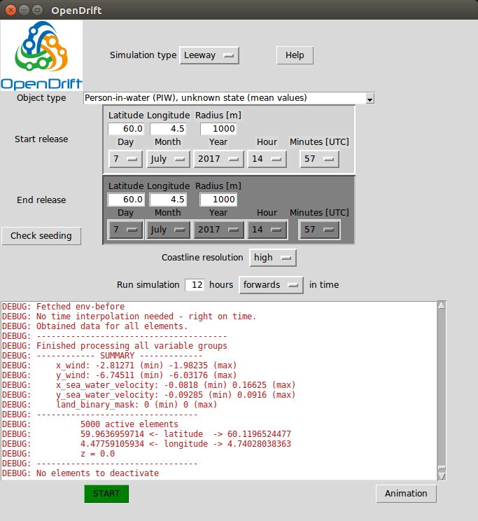
K.-F. Dagestad et al.: OpenDrift v1.0: a generic framework for trajectory modelling                                               1407

Table 1. Some existing trajectory models for various oceanic and atmospheric applications.

            Name                               Reference/URL                                   Main application
            Ariane                             Blanke et al. (1997)                            Oceanography
            BSHDmod                            Dick and Soetje (1990)                          Oil
            Connectivity Modeling System       Paris et al. (2013)                             Ocean, generic
            CIS iceberg model                  Kubat et al. (2007)                             Icebergs
            CLaMS                              McKenna et al. (2002)                           Atmospheric chemistry
            EMEP                               Simpson et al. (2012)                           Air pollution
            FLEXPART, FLEXSTRA                 www.flexpart.eu,                                Nuclear, air pollution
                                               Stohl et al. (1995)
            HYSPLIT                            Stein et al. (2015)                             Atmospheric transport
            Ladim                              Ådlandsvik and Sundby (1994)                    Plankton transport
            LAGRANTO                           Wernli and Davies (1997),                       Meteorology
                                               Sprenger and Wernli (2015)
            LAGRANTO.ocean                     Schemm et al. (2017)                            Water mass properties
            Leeway                             Breivik and Allen (2008),                       Search and rescue
                                               Allen and Plourde (1999)
            LTRANS                             Schlag and North (2012)                         Plankton (including larvae)
            MEDSLIK, MEDSLIK-II                De Dominicis et al. (2013),                     Oil
                                               Lardner et al. (1998)
            MIKE                               www.mikepoweredbydhi.com                        Ocean, generic
            MOHID                              www.mohid.com                                   Oil, sediments, water quality
            MOTHY                              Daniel (1996)                                   Oil, drifting objects
            OD3D                               Wettre et al. (2001)                            Oil
            OILMAP, SIMAP, CHEMMAP,                                                            Oil, sediments, chemical, search
                                               www.asascience.com
            MUDMAP, SARMAP                                                                     and rescue
            OILTOX                             Brovchenko et al. (2003)                        Oil
            OILTRANS                           Berry et al. (2012)                             Oil
            OSCAR                              www.sintef.no/en/software/oscar                 Oil
            OSERIT                             oserit.mumm.ac.be                               Oil, chemicals
            PARCELS                            https://github.com/OceanPARCELS/parcels         Ocean, generic
            POSEIDON-OSM                       osm.hcmr.gr                                     Oil
            PyGNOME/GNOME                      gnome.orr.noaa.gov                              Oil, generic
            SeaTrackWeb, PADM                  stw.smhi.se                                     Oil, chemicals
            SNAP                               Bartnicki et al. (2016)                         Atmospheric nuclear transport
            STILT                              www.stilt-model.org                             Atmospheric trace gases
            THREETOX                           Margvelashvily et al. (1997)                    Nuclear ocean transport
            TRACMASS                           Döös et al. (2013)                              Ocean and atmosphere, generic
            VOS                                en.ferhri.org                                   Oil

  [0.]                                                                 cast (CF) naming convention (cfconventions.org)
Available time range:                                                  should be used whenever possible. Thus, if the data source
  start: 2015-11-16 00:00:00                                           is not already following this convention (e.g. a GRIB file),
  end: 2015-11-18 18:00:00                                             the Reader should map the variable names to corresponding
  step: 1:00:00                                                        CF standard_name.
    67 times (0 missing)                                                  The given Reader class must also have implemented a spe-
Variables:                                                             cific instance of the method get_variables which is called to
  x_sea_water_velocity                                                 return data:
  y_sea_water_velocity
                                                                       >>> data = r.get_variables(["x_wind",
                                                                                  "y_wind"], x, y, z, time)
The above example shows that the created Reader object can
provide ocean surface current on a grid with 800 m pixel size          The horizontal coordinates (x,y) correspond to the native
in polar stereographic coordinates, at hourly time resolution.         projection of the Reader, which is polar stereographic in the
   To allow for generic coupling of any OpenDrift model                given example. The task of transforming from one coordinate
with any Reader, a naming convention for variables is neces-           system to another (including the rotation of vectors) is per-
sary. By convention, the commonly used Climate and Fore-               formed by common methods from the parent class, based on

www.geosci-model-dev.net/11/1405/2018/                                                       Geosci. Model Dev., 11, 1405–1420, 2018
1408 K.-F. Dagestad et al.: OpenDrift v1.0: a generic framework for trajectory modelling the widely used PROJ.4 library (proj4.org), through its and so on. This allows for a more realistic spread/diffusion Python interface pyproj. This allows OpenDrift to combine of particles than when using no or constant diffusivity. This input data from any coordinate systems, whilst keeping the functionality is particularly useful for ocean model output, implementation of new Reader classes as minimalistic and which is inherently uncertain on short timescales, due to lim- clean as possible. Further, this centralisation of code also fa- ited availability of observations for assimilation. cilitates optimisation for both performance and robustness. Whereas obtaining forcing data from 3-D Eulerian mod- The vertical coordinate (z) is by convention always in me- els is the most common in practice, Readers may obtain data tres, zero at the air/water surface and positive upwards. Thus, from any other possible source. One example is to read a time Readers providing data from sources with other vertical co- series from an American Standard Code for Information In- ordinate systems (e.g. topography following coordinates or terchange (ASCII) file of observations, e.g. from a buoy or a pressure/density levels) must take care of transforming this to weather station. Another example is to calculate forcing data metres before data are returned. This is, e.g. done by an exist- according to some analytical function. One such example is ing Reader supporting native output from the ROMS ocean included in the code repository, providing ocean current vec- model. The variable time is consistently handled as Python tors according to a “perfect circular eddy” with centre co- datetime objects within OpenDrift, with any time intervals ordinates as given to its constructor. Such analytical forcing as timedelta objects. Readers also share some common con- data fields are useful for, e.g. testing the accuracy of forward venience methods, such as plotting of geographical coverage. propagation schemes, as discussed below. Readers are, however, normally not called directly by the OpenDrift also contains some internal convenience meth- user or from specific OpenDrift instances (models) but rather ods to calculate geophysical variables from others. For exam- implicitly from the parent BaseModel class (see Sect. 2.2). ple, if a drift module requires wave height or Stokes drift, this An internal caching mechanism is implemented to minimise may be parameterised internally based on the wind velocity the amount of data to be read, which is key to improving per- if no Readers providing wave parameters are available. formance. Input data from numerical models are normally provided on a 3-D spatial grid (x, y, z) at discrete time steps, 2.2 BaseModel class which are often larger than the time steps used internally by OpenDrift models. When data are requested for a given set Functionality which is common to any trajectory model is of element positions at a given time, OpenDrift requests from described in a main class, named BaseModel. This function- the Readers’ 3-D blocks of data from the time before and af- ality includes the following: ter the given time. These 3-D blocks encompass the elements tightly, except for a buffer on each side which is large enough 1. A mechanism for configuration of a trajectory model, so that elements will stay within the coverage during the time or a specific simulation is needed. This may include step of the Reader. After 3-D blocks of data are provided adjusting the resolution of a coastline or some model- by the Reader, interpolators are generated and then reused to specific parameters concerning the movement of the el- interpolate the same data blocks onto the element positions ements. The configuration mechanism of OpenDrift is successively at each internal calculation time step, until the based upon the ConfigObj package (https://pypi.python. calculation time step reaches the latter Reader (model) time org/pypi/configobj). step. At this point, a 3-D block for the subsequent model time step is requested, and a new interpolator is generated. Due to 2. A generic method to seed elements for a simulation is this very economical access of remote data, simulations with required. See Sect. 2.3.3 for details. OpenDrift are almost as fast when obtaining data from re- mote Thredds servers, as when reading the same data from a 3. Managing and referencing a set of Readers (Sect. 2.1), local file. The interpolator mechanism is also modularised by which are called as needed to obtain forcing data dur- a dedicated class in OpenDrift, allowing independent devel- ing a simulation, are also necessary. See Sect. 2.3.2 for opment and optimisation. The default interpolation algorithm details. uses bilinear interpolation (scipy.ndimage.map_coordinates) and may also extrapolate data towards land, to avoid parti- 4. It is required to keep track of the positions and prop- cles stranding in a “no data” gap between ocean pixels from erties of all elements during a simulation and remove an ocean model and land points as determined from an inde- elements scheduled for deactivation. This is stored in pendent land mask. 2-D arrays with two dimensions, time and particle ID. Functionality exists also for reading and interpolating data Thus, the trajectory (propagation with time) of a single from ensemble models. For example, when obtaining wind element or the simulation state (all element positions from a NetCDF model file containing 10 ensemble members, and properties at a given time) is easily and quickly ob- particles number 1, 11, 21. . . will use wind from member 1 of tained as vertical or horizontal slices of the array. The the atmospheric ensemble, and particles number 2, 12, 22. . . history of data may also be written to file, as described will use wind from member 2 of the atmospheric ensemble in Sect. 2.3.6. Geosci. Model Dev., 11, 1405–1420, 2018 www.geosci-model-dev.net/11/1405/2018/
K.-F. Dagestad et al.: OpenDrift v1.0: a generic framework for trajectory modelling                                         1409

Figure 1. Flowchart of an OpenDrift simulation.

  5. Finally, the BaseModel class contains the main loop for      stance (object) of such a subclass represents a specific trajec-
     time stepping, performing necessary tasks for a simula-      tory simulation.
     tion in the correct order, as described in Sect. 2.3.5.
                                                                  2.3     Performing a simulation
   The only part missing is a description of how the elements
(e.g. objects or substance) shall be propagated and poten-
tially transformed along their trajectories under the influence   In this section, we describe and explain the general workflow
of environmental forcing data. Such application-specific de-      of a simulation with an OpenDrift model, as illustrated in the
scription is left to subclasses, yielding trajectory model in-    flowchart in Fig. 1.
stances as exemplified in Sect. 3. These subclasses thus in-
herit and may reuse any functionality from the BaseModel.
                                                                  2.3.1    Initialisation
The subclasses may also add further functionality as needed,
or overload and modify existing functionality. Thus, all nec-
essary core functionality is available by convenience but may     The first step is to import a specific OpenDrift model (sub-
be modified for flexibility. In precise terminology, OpenDrift    class of BaseModel) and to initialise an instance. The follow-
is a framework within which specific trajectory models may        ing Python statements import and initialise an instance of the
be implemented by class inheritance (subclassing). An in-         Leeway search-and-rescue model (Sect. 3.1).

www.geosci-model-dev.net/11/1405/2018/                                               Geosci. Model Dev., 11, 1405–1420, 2018
1410 K.-F. Dagestad et al.: OpenDrift v1.0: a generic framework for trajectory modelling
>>> from opendrift.models.leeway import Also the number of elements and an uncertainty radius may
Leeway be provided. Further, both position and time may be pro-
>>> l = Leeway() vided as two-element vectors to seed elements continuously
in space and time from position P1 with uncertainty radius
2.3.2 Adding Readers R1 at time T1, to position P2 with uncertainty radius R2 at
time T2. This is a common use case in search-and-rescue
If a given model requires, e.g. ocean current and atmospheric
modelling (see Breivik and Allen, 2008): a ship is known
wind as environmental forcing, we need to create and add
Reader instances which can provide these variables. Say that to have departed from position P1 at time T1, with normally
we have a Thredds server which can provide ocean currents small uncertainty radius R1, and disappeared on the way to-
and a local GRIB file which contains atmospheric winds; we wards the destination (P2), normally with larger uncertainty
can create and add these Readers to the simulation instance in position (R2) and estimated arrival time (T2). Thus, this
as follows: will track out a “seeding cone” in space and time. Another
common use case is that P1 equals P2, with T2 > T1, e.g.
>>> from opendrift.readers import reader_
simulating a continuous oil spill from a leaking well.
netCDF_CF_generic
Another built-in feature is seeding of elements within
>>> from opendrift.readers import reader_
polygons. This may, e.g. be done by providing vectors of lon-
grib
gitude and latitude:
>>> reader_current =
reader_netCDF_CF_generic.Reader( >>> l.seed_within_polygon(lon=lonvector,
’http://thredds.example.com/current.nc’) lat=latvector,
>>> reader_wind = reader_grib.Reader time=datetime(2017, 6, 25, 12),
(’winds.grib’) number=10000)
>>> l.add_readers([reader_current,
reader_wind]) This example will seed 10 000 elements with regular spac-
ing within the polygon encompassed by vectors lonvec-
For NetCDF files, it is also possible to create a single Reader
tor and latvector. Based upon this generic polygon seeding
object which merges together many files by using wildcards
method, more specific applications have been developed; see,
(∗ or ?) in the filename. This functionality is based on the
e.g. Sect. 3.2. The seeding methods may also be overloaded
NetCDF MFDataset class.
to provide customised functionality for a given module.
It is also possible to perform a simulation even with no
Readers added for one or more of the required variables. In 2.3.4 Configuration
this case, constant values may be provided; otherwise, rea-
sonable default values will be used, defaulting to zero val- OpenDrift modules share several configuration settings
ues for winds, waves and currents. For example, in the case which may be adjusted before a simulation, as well as
of having a 5-day wind forecast, but only a 3-day current some settings which are module specific. All possible set-
forecast, it is still possible to run a 5-day trajectory forecast, tings of a module may be shown with the command
where the current will be zero for the last 2 days. l.list_configspec(), of which one example is
A key feature of OpenDrift, for both convenience and ro-
drift:scheme [euler] option(’euler’,
bustness, is the possibility to provide a priority list of Read- ’runge-kutta’,
ers for a given set of variables. As an example, it is possible default=’euler’)
to specify that a high-resolution ocean model shall be used
whenever particles are within coverage in space and time, This shows that the setting drift:scheme may have one
and reverting to using another model with larger coverage or two possible values, ’euler’ or ’runge-kutta’, where the
in space and time whenever particles are outside the time or first is the default and also the present setting as indicated
spatial domain of the high-resolution model. As an important within brackets. A second-order Runge–Kutta propagation
scheme may instead be activated by the command
feature for operational setups, the backup Readers will also
be used if the first-choice model (file or URL) should not be >>> l.set_config(’drift:scheme’,
available, or if there should be any other problems, e.g. cor- ’runge-kutta’)
rupt values or files.
Another example of a configuration setting is
2.3.3 Seeding of elements coastline_action, which determines how the parti-
cles shall interact with the coastline. Possible options are
The seeding methods of OpenDrift are very flexible. The stranding, which means that particles will be deactivated
simplest case is to seed (initialise) an element at a given po- if they hit the coastline (default); previous which means
sition and time: that particles shall be moved back to their previous position
>>> l.seed_elements(lon=4.0, lat=60.0, (i.e. “waiting” at the coast until eventually moved offshore
time=datetime(2017, 6, 25, 12)) later); or none, which means that particles do not interact
Geosci. Model Dev., 11, 1405–1420, 2018 www.geosci-model-dev.net/11/1405/2018/K.-F. Dagestad et al.: OpenDrift v1.0: a generic framework for trajectory modelling 1411
with land, as for the WindBlow module as demonstrated in to various considerations such as a Bayesian update of their
Sect. 3.3. probabilities based on posterior information. Saving data to
The configuration mechanism is based on the widely used files is not a requirement, as the output of the simulations is
ConfigObj package and allows, e.g. exporting to, and import- otherwise held in memory for subsequent plotting or anal-
ing from, files of the common ’INI’ format. ysis, either interactively from within Python shell, or by a
script. A number of visualisation tools based on the Mat-
2.3.5 Starting the model run plotlib graphics library of Python are included within Open-
Drift. Some examples of both generic and module-specific
After initialisation, configuration, adding of Readers and
plotting methods are illustrated in Sect. 3.
seeding of elements, the model simulation may be started by
calling the method run:
>>> l.run(duration=timedelta(hours=48), 3 Examples of model instances
time_step=timedelta(minutes=15),
outfile=’outleeway.nc’) 3.1 Leeway (search and rescue)
This starts the main loop, as shown on the flowchart of
Fig. 1. At each time step, forcing data are obtained by all the The OpenDrift Leeway instance (OpenLeeway) is based
Readers and interpolated onto the element positions, and the on the operational search-and-rescue model of the Norwe-
model-specific update method is called to move and/or oth- gian Meteorological Institute (Breivik and Allen, 2008). The
erwise update the other element properties (e.g. evaporation model ingests a list of object classes, where each drifting
of oil elements, or growth of fish larvae) based on the envi- object has specific properties such as downwind and cross-
ronmental conditions. wind leeway (the motion due to wind) in a way similar
For the above example, the simulation will cover 48 h, to SAROPS, the operational system used by the US Coast
starting the time of the first seeded elements. The time step of Guard (see Kratzke et al., 2010, and the overview of search-
the calculation is given here as 15 min. An output time step and-rescue models by Davidson et al., 2009). These prop-
might be specified differently, with, e.g. output every hour to erties vary greatly from object to object and are based on
save memory and disk space. field work (Breivik et al., 2011, 2012a) where specific ob-
All instances of OpenDrift can be run in reverse, i.e. back- jects of relevance in search and rescue have been studied. All
wards from a final destination, by reversing the sign of the objects are assumed to be small enough that direct wave scat-
advective increment. All spatial increments due to model tering forces are insignificant. Furthermore, the Stokes drift
physics pertinent to the instance in question are calculated (Kenyon, 1969; Breivik et al., 2014, 2016) is inherently part
as normal, but the sign of the total increment, (1x, 1y, 1z), of the leeway obtained from observations. As wind-generated
is reversed and the particles are advected “backwards” over a waves have a mean direction closely aligned with the local
time step 1t. All diffusive properties are kept in the forward wind direction, it is neither practical nor desirable to disen-
sense, meaning that particles will disperse as they propagate tangle the Stokes drift from the wind drag for Leeway simu-
backwards in time. Nonlinear processes, such as evaporation lations.
of oil or capsizing of vessels, are disabled in backtracking Once an object class has been chosen and the pertinent
mode. This simple backtracking scheme is an easy-to-use al- wind and current forcing fields selected, the particles are
ternative to more complicated inverse methods, such as itera- seeded based on the available information. If the particles
tive forward trajectory modelling (Breivik et al., 2012b), and hit the coast, they stick by default. This can, however, be re-
is also much less computationally expensive. laxed so that particles detach from the coastline if the wind
direction changes.
2.3.6 Exporting model output The OpenLeeway class along with all other subclasses has
the option of being run backwards. This is a convenient fea-
In the above example, the output is saved to a CF-compliant ture in the cases where, for example, a debris field is ob-
NetCDF file (trajectory data specification), which is the de- served and the location of the accident is sought. Note that
fault output format of OpenDrift. Both particle positions and this method is fundamentally different from the BAKTRAK
any other properties, as well as configuration settings are model described by Breivik et al. (2012b) where a large num-
stored in the file. If the number of elements and time steps ber of particles were seeded in potential initial locations at
is too large to keep all data in physical memory, OpenDrift various times, and only those that ended up close to the lo-
will flush history data to the output file as needed during the cation of the observed object were kept. This is an iterative
simulation to free internal memory. The simulation may be procedure which in principle can deal with nonlinearities in
imported by OpenDrift, or independent software, for subse- the flow field as well as nonlinear behaviour of the object
quent analysis or plotting. Stored output files may also be itself (such as capsizing and swamping). Although in prin-
used as input to a subsequent OpenDrift simulation, allow- ciple this allows for a more realistic mapping of initial lo-
ing for an intermediate step where the particles are subjected cations, the difficulties associated with this iterative process
www.geosci-model-dev.net/11/1405/2018/ Geosci. Model Dev., 11, 1405–1420, 20181412 K.-F. Dagestad et al.: OpenDrift v1.0: a generic framework for trajectory modelling
mean that real-time operations are normally better off with a its decline with depth is calculated as described in
simple negative-time integration. Breivik et al. (2016).
OpenLeeway is used operationally at Norwegian Meteoro-
– Oil elements at the ocean surface are moved with an
logical Institute and is also currently being implemented as
additional factor of 2 % (configurable) of the wind. To-
the operational search-and-rescue model for the Joint Rescue
gether with the Stokes drift (typically 1.5 % of the wind
Coordination Centres (JRCC) of Norway.
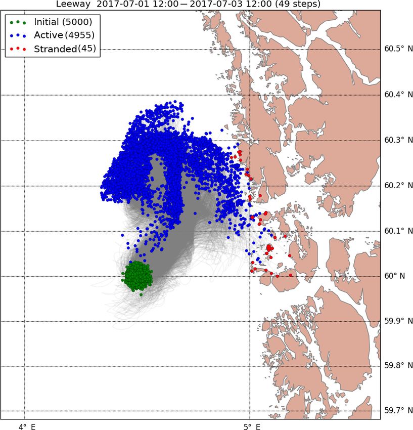
The following lines of Python code illustrate a complete at the surface), this sums up to the commonly found em-
working example of running an OpenLeeway simulation: pirical value of 3.5 % of the wind (Schwartzberg, 1971).
The physical mechanism behind this wind drift factor is
from opendrift.readers import reader_netCDF_
not obvious and is discussed in Jones et al. (2016).
CF_generic
from opendrift.models.leeway import Leeway The above three drift components may lead to a very
l = Leeway() # Creating a simulation object strong gradient of drift magnitude and direction in the up-
# Wind field per few metres of the ocean. For this reason, it is also of
reader_wind = reader_netCDF_CF_generic. critical importance to have a good description of the vertical
Reader(’http://thredds.met.no/thredds/ oil transport processes, which in OpenOil are the sum of the
dodsC/meps25files/meps_det_pp_2_
following factors:
5km_latest.nc’)
# Ocean model data – If the vertical ocean current velocity is available from a
reader_ocean = reader_netCDF_CF_generic. Reader, the oil elements will follow it. This part of the
Reader(’http://thredds.met.no/thredds/ movement is, however, often negligible compared to the
dodsC/sea/norkyst800m/1h/aggregate_be’) processes below.
l.add_reader([reader_wind, reader_ocean])
# Seed elements at defined position and time – Oil elements at the surface, regarded as being in the state
objType = 26 # Life-raft, no ballast of an oil slick, may be entrained into the ocean by break-
l.seed_elements(lon=4.5, lat=60.0, ing waves. Presently, OpenOil contains two different
radius=1000, number=5000, parameterisations of this entrainment rate, from which
time=datetime(2017,7,1,12), the user can chose as part of configuration (see below):
objectType=objType) Tkalich and Chan (2002) and Li et al. (2017). The en-
# Running the model 48 hours ahead
trainment depends on both the wind and wave (break-
l.run(duration=timedelta(hours=48))
# Print and plot results
ing) conditions and also on the oil properties, such as
print viscosity, density and oil–water interfacial tension.
l.animation(filename=’leeway_example.mp4’) – Buoyancy of droplets is calculated according to empir-
l.plot(filename=’leeway_example.png’)
ical relationships and the Stokes law of Tkalich and
The final plotting command yields Fig. 2. The coastline Chan (2002), dependent on ocean stratification (calcu-
shown is from the GSHHS database (Wessel and Smith, lated from temperature and salinity profile, normally
1996), which is the default option used to check strand- read from an ocean model), oil and water viscosities and
ing in OpenDrift. This coastline is, however, interfaced densities. Also, the buoyancy is strongly dependent on
to OpenDrift as a regular Reader (Sect. 2.1) and can be the oil droplet size (diameter), of which two parameter-
replaced by any other Reader providing the CF variable isations are available: one is a generic power law, with
land_binary_mask. This allows performing simulations in droplets between a minimum and maximum diameter,
narrow bays or lakes where even the full-resolution GSHHS and a configurable exponent where −2.3 corresponds
coastline is too coarse. to the classical work of (Delvigne and Sweeney, 1989).
The second option for droplet size spectrum is a “mod-
3.2 OpenOil (oil drift) ern” approach by Johansen et al. (2015), where a log-
normal droplet spectrum is calculated explicitly based
OpenOil is a full-fledged oil drift model, bundled within the on wave height and oil properties such as viscosity, den-
OpenDrift framework. As a model, it has been developed sity, interfacial tension and surface film thickness.
from scratch but is based on a selection of parameterisations
of oil drift as found in the open research literature. With re- – In addition to the wave-induced entrainment, the oil el-
gard to horizontal drift, three processes are considered: ements are also subject to vertical turbulence through-
out the water column, as parameterised with a numeri-
– Any element, whether submerged or at the surface,
cal scheme described in Visser (1997). This scheme is
drifts along with the ocean current.
generic within OpenDrift and is also used by the Pelag-
– Elements are subject to Stokes drift corresponding to icEgg module for ichthyoplankton (Sect. 3.4). Only the
their actual depth. Surface Stokes drift is normally ob- properties specific to oil, or plankton, are coded in the
tained from a wave model (or by any Reader), and respective classes (modules).
Geosci. Model Dev., 11, 1405–1420, 2018 www.geosci-model-dev.net/11/1405/2018/K.-F. Dagestad et al.: OpenDrift v1.0: a generic framework for trajectory modelling 1413
Figure 2. Output from the Leeway example of Sect. 3.1. Green dots are the initial positions of the elements (life rafts), grey lines are
trajectories, and blue dots are positions at the end of the simulation. Red dots indicate elements which have hit land (stranded).
In addition to the vertical and horizontal drift, weath- a corresponding oil name from the NOAA database. How-
ering of the oil also has to be considered. While pa- ever, whereas key features and functionality is shared among
rameterisations of weathering might also be imple- OpenDrift modules, each module (or group of modules) may
mented directly within the OpenDrift framework, the add specific functionality. For example, for OpenOil, it is
OpenOil module instead interfaces with the already possible to initialise the simulations with an oil slick as read
existing OilLibrary software developed by NOAA from a file containing contours, either a shapefile or the Ge-
ography Markup Language (GML) format/specification, as
(https://github.com/NOAA-ORR-ERD/OilLibrary). The used by the European Maritime Safety Agency (EMSA):
NOAA OilLibrary is also open-source and written in
Python, so integration is straightforward. In addition to >>> o.seed_from_gml("RS2_20151116_002619_
state-of-the-art parameterisations of processes such as evap- SCNB_HH_Oil.gml", num_elements=2000)
oration, emulsification and dispersion, this software contains >>> o.plot()
a database of measured properties of almost 1000 oil types
from around the world. As oils from different sources/wells where o is the oil drift simulation object. The last command
have vastly different properties, such a database is of produces the plot shown in Fig. 3.
vital importance for accurate results. The same OilLibrary OpenOil also has module-specific configuration settings.
is also used by the NOAA oil drift model PyGNOME The following commands specify that the oil entrainment
(https://github.com/NOAA-ORR-ERD/PyGnome), where rate shall be calculated according to Li et al. (2017), and the
oil droplet size spectrum shall be calculated according to Jo-
it is replacing the original ADIOS oil library (Lehr et al.,
hansen et al. (2015).
2002). PyGNOME includes also more processes not (yet)
included in OpenOil, such as dissolution, and adding of >>> o.set_config(’wave_entrainment:
dispersants. entrainment_rate’,
To run an OpenOil simulation, one could reuse the exact ’Li et al. (2017)’)
code as for the Leeway example of Sect. 3.1, only replacing >>> o.set_config(’wave_entrainment:droplet_
the name of the imported module (OpenOil instead of Lee- size_distribution’,
way) and replacing the objectType property of Leeway with ’Johansen et al. (2015)’)
www.geosci-model-dev.net/11/1405/2018/ Geosci. Model Dev., 11, 1405–1420, 20181414 K.-F. Dagestad et al.: OpenDrift v1.0: a generic framework for trajectory modelling
required_variables = [’x_wind’, ’y_wind’]
def update(self):
self.update_positions(
self.environment.x_wind,
self.environment.y_wind)
Because all common functionality is inherited from the
main class, the WindBlow model only needs to address its
own specific needs. It will use elements without any other
properties except for position (PassiveTracer), and the only
forcing needed to move the elements is wind, whose vector
components are named x_wind and y_wind in CF terminol-
ogy. The update() method which is called at each time step
simply advects all elements with the wind velocity at their
respective locations. The wind might be provided by any
Reader (Sect. 2.1). The WindDrift module may be run with
an even more simplified form of the code example found in
Sect. 3.1: the WindDrift class has to be imported, no Reader
for ocean current is needed, and there is no object category
Figure 3. Oil drift simulation initialised by seeding 2000 oil el-
to specify.
ements within contours of an oil slick as observed from satellite Clearly, an air parcel in the real atmosphere will also be
(Radarsat2). The contour is imported from a Geography Markup subjected to updrafts and diffusion, and will with time rise or
Language (GML) file produced by Kongsberg Satellite Services fall, but the example serves to demonstrate how little is re-
(KSAT). quired to develop a new subclass of OpenDrift. The model
may be made more sophisticated by adding, e.g. vertical
wind (upward_air_velocity) and turbulence parameters to the
Adjusting configuration this way is convenient for sensitivity list of required variables, and adding corresponding parame-
studies, where one component is changed for two otherwise terisations of how to use this information for the advection.
identical simulations.
After the simulation is finished, the generic plot command 3.4 Other modules
may be used to produce a map with trajectories as shown
in Fig. 2. However, more specific plotting methods are also In addition to the models described above, some other mod-
available. The command o.plot_oil_budget() plots ules are bundled within the OpenDrift repository, as illus-
an oil budget as shown in Fig. 4. trated in Fig. 6:
The vertical distribution of the ele-
ments can be plotted with the command – OceanDrift is a basic module for tracking, e.g. water
o.plot_vertical_distribution(), generat- masses or passive tracers. Stokes drift is included, if
ing output as shown in Fig. 5. This method is shared provided by a Reader. A wind drift factor may also be
among three-dimensional modules and may also be used for specified, allowing an additional wind drag at the sur-
simulations with, e.g. the PelagicEgg module (Sect. 3.4). face, e.g. for simulation trajectories of various ocean
drifting buoys (Dagestad and Röhrs, 2018).
3.3 WindBlow (atmospheric transport)
– PelagicEgg is a module for transport of pelagic ichthy-
As an example of a minimalistic trajectory model, we also oplankton. This module contains quite basic function-
include the instance WindBlow, which simply calculates ality with identical transport mechanisms as in Röhrs
the propagation of a passive particle subject to a two- et al. (2014), including the vertical turbulent scheme
dimensional wind field. The code below is the complete and (Sect. 3.2) which is of key importance for most pelagic
fully functional WindDrift module. plankton applications. Although a fully working a mod-
ule, users with specialised needs (e.g. a specific bio-
# WindBlow module code from opendrift.
models.basemodel
logical species) can customise the drift and behaviour
import OpenDriftSimulation from opendrift. parameterisations by modifying or adding parameteri-
elements.passivetracer import PassiveTracer sations in the PelagicEgg module, such as larval be-
haviour. Some users have interfaced this module with
class WindBlow(OpenDriftSimulation): existing Fortran code, e.g. for calculation of sunlight-
ElementType = PassiveTracer dependent behaviour; see, e.g. Kvile et al. (2018) and
Geosci. Model Dev., 11, 1405–1420, 2018 www.geosci-model-dev.net/11/1405/2018/K.-F. Dagestad et al.: OpenDrift v1.0: a generic framework for trajectory modelling 1415
Figure 4. Plot of the time evolution of the oil budget of a 24 h simulation with OpenOil. Of 500 kg oil initially at the ocean surface, about
20 % is seen to evaporate within the 24 h. The amount of oil submerged due to wave action and ocean turbulence varies with the wind
and wave conditions, with more oil resurfacing when wind decreases after about 7 h. After about 18 h, some of the oil is seen to hit the
coastline. These results are for the oil type “Martin Linge crude”; very different results could be obtained if using another oil type for the
same geophysical conditions.
tested and shown to provide identical output for identi-
cal input/forcing.
A module for drift of icebergs (OpenBerg, not yet included
in repository) has been developed by Ron Saper at Carleton
University with partial funding from ASL Environmental
Sciences of Victoria, Canada, and with data support from
the Canadian Ice Service (personal communication, 2017).
Two different iceberg drift forecasting approaches are be-
ing tested. One approach uses a drag formulation to calcu-
late wind and water drag forces. The challenge with this ap-
proach is that the trajectories are very sensitive to underwa-
Figure 5. Vertical profile of the amount of (oil) elements. The bot- ter draft/shape and suitable drag coefficients, of which infor-
tom bar is an interactive slider, which the user can pull left/right to mation is rarely available. The second approach predicts and
see the time variation of the vertical distribution. subtracts the wind and tidal components of the drift, and then
analyses the residual for extrapolation an appropriately short
time into the future. Finally, wind and tidal components are
Sundby et al. (2017). A pure Python version of the sun- added back in to produce a trajectory forecast. The first ver-
light module is available and will be included in a future sion of OpenBerg does not include thermodynamic effects
version of OpenDrift. (melting) which are important longer timescales from weeks
to months.
– ShipDrift is a module for predicting the drift of ships Drift of marine plastics, including microplastics, is an im-
larger than 30 m, where the effect of waves has to be portant application not covered by modules included with the
calculated explicitly, and not implicitly with the wind OpenDrift repository version 1.0. However, as most of the
drift as in the Leeway module. This module is based needed infrastructure is already provided, including a ver-
on Sørgård and Vada (2011). A previous version pro- tical mixing scheme, a user with knowledge of the relevant
grammed in the C programming language has been physics and basic Python programming should be able to im-
used operationally at MET Norway for 15 years but is plement such a module with moderate efforts. However, there
now replaced by the OpenDrift version, which has been is no upper limit to the complexity of any module.
www.geosci-model-dev.net/11/1405/2018/ Geosci. Model Dev., 11, 1405–1420, 20181416 K.-F. Dagestad et al.: OpenDrift v1.0: a generic framework for trajectory modelling
Figure 6. Illustration of how OpenDrift modules for specific applications (white boxes) inherit common functionality from the core module.
This includes functionality to interact with Readers for obtaining forcing data. Subclassing (inheritance) allows, e.g. both the OpenOil and
PelagicEgg models to share further 3-D-functionality through subclassing the OpenDrift3D class. The boxes with solid boundaries illustrate
existing modules bundled with the OpenDrift repository, whereas dashed boundaries indicate planned modules. The green box illustrates that
OpenOil (oil drift model) utilises functionality from a third-party library, the NOAA OilLibrary.
4 Test suite and example scripts 5 Graphical user interfaces
OpenDrift contains a broad set of automatic tests (Python Although running OpenDrift modules with Python scripts
unittest framework) which can be run by the user to assure (see, e.g. Sect. 3.1) is the most flexible and powerful, a basic
that all calculations are performed correctly on the local ma- graphical user interface (GUI) is also included in the repos-
chine. The tests cover both basic calculations, such as inter- itory. A screenshot is shown in Fig. 7. The GUI allows to
polation and rotation of vectors from one spatial reference select a module and an object type or medium (e.g. oil type)
system (SRS) to another, but also more extensive integration corresponding to the module, and then a seeding location and
tests, performing full simulations with the modules to ver- time. The simulation is started by clicking the “START” but-
ify that an expected numerical result is obtained. Also, very ton, and plots and animation of the output is available after
importantly, the tests are also run automatically on a variety the simulation and also saved to a NetCDF file. The GUI will
of machine configurations, using the Travis Continuous In- obtain forcing data through a provided list (configurable) of
tegration (CI) framework (https://travis-ci.org). This ensures Thredds servers with global coverage, so there is no need for
that OpenDrift calculations remain accurate and correct with the user to obtain and download large amounts of model in-
both old and new versions of the various required libraries put in advance. Although presently with only basic function-
(e.g. NumPy), and that existing functionality is not broken ality, the GUI is in operational use at MET Norway, where
as new functionality is added. For version 1.0 of OpenDrift, it is tested daily by meteorologists on duty as part of the oil
64 % of the code is covered by the unit tests, as reported by spill and search-and-rescue preparedness system.
the Coveralls tool (coveralls.io). In addition to the native GUI, a web interface has also been
A user manual of OpenDrift is kept alongside the code developed for remote access without need for any local in-
repository on the wiki pages of GitHub (https://github.com/ stallation. This is based on communication with OpenDrift
OpenDrift/opendrift/wiki), facilitating a dynamic description through a web processing service (WPS) developed at MET
to evolve with the code, instead of diverting from it. Many Norway (not included in the repository). Independently, a
example scripts (40 in version 1.0) are also provided in the WPS for the Leeway module has also been developed and
repository along with the needed input forcing data, illustrat- implemented at the Swedish Met Office (SMHI). A generic
ing a variety of real-life use cases. The examples can easily and configurable WPS to be included in the repository is
be modified and adapted, allowing a soft learning curve. planned for the future.
OpenDrift also comes with a set of handy command line
tools, such as readerinfo.py, which may be used to easily in-
spect the contents and coverage of potential forcing fields. 6 Discussion and conclusions
The following shell command produces the same output as
the example of Sect. 2.1, where the switch ’-p’ also displays Several offline trajectory models exist to predict the trans-
a plot of the geographical coverage: port and transformation of various substances and objects in
the ocean or in the atmosphere. OpenDrift is an open-source
$ readerinfo.py ocean_model_output.nc -p Python framework aiming at extracting anything which is
Geosci. Model Dev., 11, 1405–1420, 2018 www.geosci-model-dev.net/11/1405/2018/K.-F. Dagestad et al.: OpenDrift v1.0: a generic framework for trajectory modelling 1417 Figure 7. Screenshot of the graphical user interface included with OpenDrift. common to all such trajectory models in a core library, and core provides even greater flexibility to the user in that it is combining this with a clean and generic interface for de- easy to modify existing modules, or even write new mod- scribing any processes which are application specific. Sev- ules from scratch. Several users have already developed or eral examples of such specific modules are bundled with the adjusted modules for their specific purpose and added use- OpenDrift code repository and serve as ready-to-use trajec- ful contributions to the OpenDrift core (Sundby et al., 2017; tory models. This includes an oil drift model (OpenOil), a Kvile et al., 2018). search-and-rescue model (Leeway) and a model for predict- Whereas flexibility is important for scientific studies, ing the drift and transformation of ichthyoplankton (Pelag- OpenDrift is also designed for performance and robustness icEgg). Interfaces (Readers) towards the most common for- and is in daily use for operational emergency response sys- mats of forcing data (e.g. NetCDF and GRIB) are also in- tems at the Norwegian Meteorological Institute. Being able cluded, allowing any of the modules to be forced by data to use the same tool in both cases facilitates rapid transition from a combination of files and other sources, including re- of the latest research results into operations. mote Thredds servers. The concept of Readers is also modu- The efficiency of the code has been optimised to the point larised, allowing a scientist or programmer to easily develop that more time is normally spent on reading the forcing data an interface towards any other specific source of forcing data, from disk (or a URL) than on performing actual calculations. e.g. an ASCII file containing in situ observations from a buoy Computational performance similar to compiled languages or weather station, or ocean currents from HF-radar systems (Fortran or C) is obtained by, e.g. using primarily NumPy in a specific binary format. arrays for calculations (avoiding the slower MaskedArray A built-in configuration mechanism provides flexibility to class) and avoiding “for loops”. A typical emergency sim- the operation of the OpenDrift modules. However, the fact ulation with the Leeway model with 5000 elements and 48 h that the application-specific processes of these modules are duration takes on the order of 1 min. A corresponding simu- separated from the technical complexities of the OpenDrift lation with OpenOil takes about 3–5 min, primarily because www.geosci-model-dev.net/11/1405/2018/ Geosci. Model Dev., 11, 1405–1420, 2018
1418                                   K.-F. Dagestad et al.: OpenDrift v1.0: a generic framework for trajectory modelling

more layers of ocean model data have to be read from disk, in      Acknowledgements. Knut-Frode Dagestad, Johannes Röhrs and
contrast to the Leeway simulation which only needs the sur-        Øyvind Breivik gratefully acknowledge support from the Joint
face current. A typical 1-year simulation of 20 000 drifting       Rescue Coordination Centres through the project OpenLeeway
cod eggs (developing into larvae) takes about 4 h on a reg-        and the Research Council of Norway through the CIRFA (grant
ular desktop computer (Kvile et al., 2018). The OpenDrift          no. 237906) and RETROSPECT (grant no. 244262) projects. The
                                                                   Norwegian Clean Seas Association (NOFO) and the Norwegian
code is presently not parallelised. However, given that most
                                                                   Coastal Administration have been instrumental in their support and
time is spent on reading data from disk, some further per-         testing of the software during the development phase.
formance gain could possibly be achieved by, e.g. reading in
parallel data from different input files (e.g. ocean model and     Edited by: Robert Marsh
atmospheric model) or by reading input data for the follow-        Reviewed by: two anonymous referees
ing time step in parallel to performing calculations.
   Another great benefit of the modularity provided by Open-
Drift is the ability to perform sensitivity tests by varying one
component while keeping everything else constant. Much
can be learnt from performing two otherwise identical sim-
                                                                   References
ulations with, e.g. input from two different Eulerian models,
or by using two different parameterisations of some process.       Ådlandsvik, B. and Sundby, S.: Modelling the transport of cod lar-
Further, consistency is also provided by the possibility of          vae from the Lofoten area, ICES J. Mar. Sci. Symp., 198, 379–
handling, e.g. overlap of fish eggs and oil with the same forc-      392, available at: https://www.scienceopen.com/document?vid=
ing and numerical scheme. Traditionally, it might be difficult       53b16ebf-bddc-4332-8719-1bb180e1cdaa (last access: 9 April
to draw conclusions by comparing the output from different           2018), 1994.
trajectory models, as the differences depend on many factors,      Allen, A. and Plourde, J. V.: Review of Leeway: Field Experiments
such as interpolation schemes and numerical algorithms.              and Implementation, US Coast Guard Research and Develop-
   The modules presently included with OpenDrift will be             ment Center, 1082 Shennecossett Road, Groton, CT, USA, Tech.
improved in the future, in particular by validation against          Rep. CG-D-08-99, available through: http://www.ntis.gov (last
available relevant observations. Among the general prob-             access: 9 April 2018), 1999.
                                                                   Bartnicki, J., Amundsen, I., Brown, J., Hosseini, A., Hov, O.,
lems which require more attention, is properly describing
                                                                     Haakenstad, H., Klein, H., Lind, O. C., Salbu, B., Szacin-
and quantifying the very strong vertical gradients of horizon-
                                                                     ski Wendel, C. C., and Ytre-Eide, M. A.: Atmospheric
tal drift often found in the upper few metres of the ocean,          transport of radioactive debris to Norway in case of a
as result of a delicate balance between ocean currents and           hypothetical accident related to the recovery of the Rus-
Stokes drift, as well as the direct wind drift affecting objects     sian submarine K-27, J. Environ. Radioactiv., 151, 404–416,
and substances at the very ocean surface. This vertical gra-         https://doi.org/10.1016/j.jenvrad.2015.02.025, 2016.
dient of forcing is highly important for drift of, e.g. oil and    Berry, A., Dabrowski, T., and Lyons, K.: The oil
chemicals, plankton and microplastics. This implies further          spill model OILTRANS and its application to the
that having accurate parameterisations of the vertical trans-        Celtic Sea, Mar. Pollut. Bull., 64, 2489–2501,
port processes (wave entrainment, buoyancy and ocean tur-            https://doi.org/10.1016/j.marpolbul.2012.07.036, 2012.
bulence) is also very important. For example, a key factor         Blanke, B., Raynaud, S., Blanke, B., and Raynaud, S.: Kine-
                                                                     matics of the Pacific Equatorial Undercurrent: An Eulerian
for successful simulation of the drift of observed oil slicks
                                                                     and Lagrangian Approach from GCM Results, J. Phys.
in Jones et al. (2016) was to incorporate a vertical mixing
                                                                     Oceanogr., 27, 1038–1053, https://doi.org/10.1175/1520-
scheme developed for fish eggs (Sundby, 1983; Thygesen               0485(1997)0272.0.CO;2, 1997.
and Ådlandsvik, 2007; Ådlandsvik and Sundby, 1994) into            Breivik, Ø. and Allen, A. A.: An operational search and rescue
the oil drift model OpenOil.                                         model for the Norwegian Sea and the North Sea, J. Marine Syst.,
                                                                     69, 99–113, https://doi.org/10.1016/j.jmarsys.2007.02.010,
                                                                     2008.
Code availability. OpenDrift     is     housed    on    GitHub:    Breivik, Ø., Allen, A. A., Maisondieu, C., and Roth,
https://github.com/OpenDrift/opendrift.    The     accompanying      J. C.: Wind-induced drift of objects at sea: The lee-
wiki pages contain installation instructions, documentation and      way field method, Appl. Ocean Res., 33, 100–109,
examples. Version 1.0 of OpenDrift is registered with Zenodo:        https://doi.org/10.1016/j.apor.2011.01.005, 2011.
https://doi.org/10.5281/zenodo.845813. OpenDrift has been tested   Breivik, Ø., Allen, A., Maisondieu, C., Roth, J.-C., and
on both Linux, Mac and Windows platforms. Version 1.0 requires       Forest, B.: The Leeway of Shipping Containers at Dif-
Python 2.7 and is not adapted for Python 3. The OpenDrift            ferent Immersion Levels, Ocean Dynam., 62, 741–752,
framework is distributed under a GPLv2 license.                      https://doi.org/10.1007/s10236-012-0522-z, 2012a.
                                                                   Breivik, Ø., Bekkvik, T. C., Ommundsen, A., and Wettre, C.: BAK-
                                                                     TRAK: Backtracking drifting objects using an iterative algorithm
                                                                     with a forward trajectory model, Ocean Dynam., 62, 239–252,
                                                                     https://doi.org/10.1007/s10236-011-0496-2, 2012b.

Geosci. Model Dev., 11, 1405–1420, 2018                                              www.geosci-model-dev.net/11/1405/2018/
You can also read