MODELING CHOICE INTERDEPENDENCE IN A SOCIAL NETWORK

Page created by Tyrone Hogan

Society

English

Like
Share
Embed
Fullscreen
Slides
Download HTML
Download PDF
Abuse

←

→

Page content transcription

If your browser does not render page correctly, please read the page content below

MODELING CHOICE INTERDEPENDENCE IN A SOCIAL NETWORK

MODELING CHOICE INTERDEPENDENCE IN A SOCIAL NETWORK

                     Jing Wang, Anocha Aribarg, and Yves F. Atchadé *
                                         July 2013

                              Forthcoming, Marketing Science

*
 Jing Wang is specialist in Asia-Pacific marketing and sales practice of McKinsey & Company,
233 Taicang Rd, Shanghai, China 200020. E-mail: jingwang16@gmail.com. Anocha Aribarg is
Associate Professor of Marketing at Stephen M. Ross School of Business, University of
Michigan, 701 Tappan Street, Ann Arbor, Michigan 48109. E-mail: anocha@umich.edu. Yves F.
Atchadé is Associate Professor of Statistics at the Department of Statistics, University of
Michigan, 454 West Hall, 1085 South University Avenue, Ann Arbor, Michigan 48109. E-mail:
yvesa@umich.edu. The paper is based on the first author’s dissertation. We thank Stefan
Witwicki for his assistance in JAVA and Flash programming to facilitate our data collection
process. We thank Natasha Zhang Foutz for great comments for our paper. Finally, we thank the
review team for providing us with valuable comments and directions for the paper.

                                                                                            1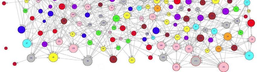

ABSTRACT

This paper investigates how individuals’ product choices are influenced by the product choices

of their connected others, and how the influence mechanism may differ for fashion versus

technology-related products. We conduct a novel field experiment to induce and observe choice

interdependence in a closed social network. In our experiment, we conceptualize individuals’

choices to be driven by multi-attribute utilities and measure their initial attribute preferences

prior to observing their choice interdependence, as well as collecting network information. These

design elements help alleviate concerns in identifying social interaction effects from other

confounds. Given that we have complete information on choices and their sequence, we use a

Discrete-time Markov Chain (DMC) model. Nonetheless, we also use a Markov Random Field

(MRF) model as an alternative when the information on choice sequence is missing. We find

significant social interaction effects. Our findings show that while experts exert asymmetrically

greater influences for a technology-related product, popular individuals exert greater influences

for a fashion-related product. In addition, we find choices made by early decision makers to be

more influential than choices made later for the technology-related product. Finally, using the

MRF with snapshop data can also provide good out-of-sample prediction for a technology-

related product.

Keywords: social interactions, social network, social influence, homophily, conjoint experiment,

Markov random field

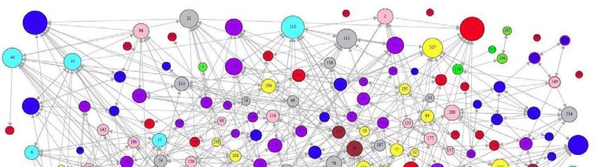
Researchers have long recognized the impact of social interactions among individuals in

a social network on their preference evolution and product adoptions. The rapid growth of social

networking websites has facilitated social interactions to an unprecedented level. In addition to

encouraging users to maintain current and build new connections on the site, Facebook

automatically passes along information about users’ site activities to their friends. For instance,

when users become a fan of a brand page or respond to an interactive ad on the site, their friends

receive a notification. These notifications are sent with the expectation that they may influence

others. Social interaction effects are also undoubtedly prevalent in offline contexts. Individuals’

decisions to purchase a hybrid vehicle, for example, may be influenced by recommendations

from their neighbors. Teenagers’ decisions to purchase certain brands of jeans can be influenced

by observing their peers’ choices. In this paper, we examine social interactions in a multi-

attribute choice context where we conceptualize choice interdependence in a social network as

being driven by individuals’ preference shifts induced by social interactions after controlling for

their initial preferences.

Although extant research has attempted to measure social interaction effects (e.g., Nair,

Manchanda, and Bhatia 2010; Nam, Manchanda, and Chintagunta 2010; Tucker 2008), it does

not recognize that such effects may arise from different types of social influence. Prior

behavioral research (Bearden and Etzel 1982; Burnkrant and Cousineau 1975; Deutsch and

Gerard 1955) distinguishes a value-expressive from an informational social influence. While an

informational influence is driven by an individual’s goal to gain more knowledge, a value-

expressive influence is driven by someone’s goal to maintain and enhance their self-perception

or identity in relation to their peers. Given different goal orientations, consumers rely more on

the credibility of the source of influence when it comes to an informational influence and more

on desirable characteristics of the source when it comes to a value-expressive influence

(McGuire 1969). Given that we expect an informational influence to play a more important role

for a technology-related product and a value-expressive influence for a fashion-related product,

we examine how experts (i.e., more credible) versus popular (i.e., with a more desirable

characteristic) individuals are asymmetrically more influential for technology-related versus

fashion-related products. In addition, previous research suggests that two distinct groups of

influentials and imitators may play different roles in the diffusion of innovations (Van den Bulte

and Joshi 2007). That is, influentials tend to be opinion leaders (Katz and Lazerfeld 1955) and

early adopters who influence, but are not or to a lesser degree influenced by, imitators. Provided

with information about the sequence of choices, we also assess whether individuals are more

influenced by the choices made by early decision makers, as opposed to the choices made later.

Prior research has attempted to identify the causal effects of social interactions

(Hartmann et al. 2008; Manski 1993, 2000; Moffitt 2001). With observational data, social

interactions are likely confounded with homophily or endogenous group formation, correlated

unobservables, and simultaneity. We propose a novel conjoint experiment for studying social

interactions that helps alleviate these endogeneity concerns. Specifically, we examine choice

interdependence in a social network and conceptualize consumer choices to be driven by multi-

attribute utilities. We conduct a two-stage choice experiment with a pre-influence stage, followed

by a post-influence stage. The experiment also involves two product categories: a fashion-related

one and a technology-related one. In the pre-influence stage, we use a conjoint choice

experiment to measure each participant’s initial preferences for different product attributes that

govern the utilities of the product choices. We also collect information about their social

connections within a closed social network. In the post-influence stage, we conduct an incentive-

aligned choice experiment to induce and observe choice interdependence within the network.

This experimental design helps us to identify preference shifts as a result of social interactions

separately from initial preferences.

To study choice interdependence and identify the social interaction effects, it is also

desirable for researchers to observe both individual choices and the sequence of choices

(complete data). We fit a discrete-time Markov chain (DMC) model to the complete data.

However, oftentimes researchers do not keep records of the sequence due to a capacity

constraint, or in offline contexts it may not even be feasible to observe the choice sequence. In

these situations, researchers have to work with cross-sectional data where realized choices are

recorded only at a particular time point (snapshot data). Given their theoretical connection, we

demonstrate how researchers can use a Markov random field (MRF) model as an alternative to a

DMC model when only snapshot data are available. Both DMC and MRF models are appropriate

for modeling choice interdependence in a social network because both models properly account

for the dependence structure in the data (i.e., the joint probability of individual choices).

Controlling for individuals’ heterogeneous initial preferences, we find significant social

interaction effects based on both the DMC and MRF models. Our findings suggest that, on the

one hand, popular individuals (i.e., those with more connections) exert greater influence for a

fashion-related product where value-expressive influence is more prominent. On the other hand,

experts exert greater influence for a technology-related product where informational influence

dominates. We also find that individuals who make choices earlier are more influential in the

technology-related product category. This result alludes to the opinion leadership of early

decision makers for this product category. Finally, our model comparison shows good out-of-

sample predictive performance of the MRF model for the technology-related product.

The contribution of our paper is threefold. First, we assess how different types of

influences, informational versus value-expressive, lead experts versus popular individuals to

asymmetrically exert greater influence, respectively, for technology-related versus fashion

related-products. We also examine the potential disproportionate influence of early decision

makers. Second, coupled with network information, we demonstrate how researchers can use a

two-stage conjoint choice experiment, which is conceptualize based on the multi-attribute utility

framework (Keeney and Raiffa 1993), to identify individual preference shifts induced by social

interactions after controlling for their initial preferences. Our approach helps mitigate the

endogeneity concern. Finally, given that we use the DMC to model choice interdependence when

the information on both choices and their sequence is available, we examine how the

theoretically connected MRF model can be used as an alternative when the sequence information

is missing—a common occurrence in most online and offline situations.

The paper is structured as follows. We begin with the literature review in relation to our

conceptual framework and then present our modeling framework. This is followed by a

description of our experimental design and data collection procedure. Our empirical analysis

section includes: i) descriptive statistics of the participants and their social network; ii) the

analysis of individual-specific initial preferences; iii) the detailed model specification and

estimation procedure; iv) model comparison; and v) estimation results. The discussion section

concludes our paper.

LITERATURE REVIEW AND CONCEPTUAL FRAMEWORK

There is a sizable body of literature on social interaction effects (also referred to as peer,

neighborhood, and social contagion effects) in the fields of economics, sociology, and marketing.

In economics, the primary focus is on identifying an “active” social interaction that gives rise to

a social multiplier using observational data (Brock and Durlauf 2001; Manski 1993, 2000).

Hartmann et al. (2008) distinguish active from passive social interactions; the former involves

two individuals’ actions being simultaneously affected by the actions of the other and resolved as

an equilibrium outcome (e.g., Hartman 2010) while the latter treats the impact of an individual’s

action on the other’s action as being sequential in nature. Although the concept of active social

interactions originates in sociology (Granovetter 1978; Schelling 1971), the majority of work in

this discipline does not hinge upon an equilibrium assumption (i.e., focus on passive social

interactions), and the emphasis is placed on how the structure of individuals’ social network

affects how social interactions propagate information diffusion in the network (Granovetter

1973; Katz and Lazarfeld 1955; Watts and Dodds 2007). Comparing to sociology, not much

attention has been paid to the structure of a social network in the economic literature. Early

research in economics and sociology mainly proposes theoretical frameworks to characterize the

mechanism of social interactions without corroborating empirical evidence.

       Despite no explicit attempt to model social interactions, the marketing literature has long

recognized their role (i.e., influentials vs. imitators) in the diffusion of innovations (Bass 1969;

Van den Bulte and Stremersch 2004; Van den Bulte and Wuyts 2007). With the availability of

observational data especially in online contexts, research in marketing explicitly links social

interactions to firm performance and product adoptions (Godes et al. 2005; Hartmann et al.

2008). On the one hand, some researchers have examined the effects of aggregate word-of-

mouth (Chen, Wang and Xie 2011; Chevalier and Mayzlin 2006; Godes and Mayzlin 2004; Zhu

and Zhang 2010), online viral marketing activities (De Bruyn and Lilien 2008; Toubia, Freud,

and Stephen 2011), and online community participation (Algesheimer et al. 2010; Manchanda,

                                                                                                       7

Packard, and Pattabhiramaiah 2013; Stephen and Toubia 2010) on aggregate sales. On the other

hand, others attempt to establish the casual effects of social interactions on adoption decisions at

the individual level (Nair, Manchanda and Bhatia 2010; Nam, Manchanda, and Chintagunta

2010; Tucker 2008; Zhang 2010). A few researchers examine social interactions in a multi-

attribute utility framework1 (Narayan, Rao, and Saunders 2011; Yang and Allenby 2003) or

explicitly collect network information (Nair, Manchanda, and Bhatia 2010; Narayan, Rao, and

Saunders 2011; Reingen et al. 1984). In studying choice interdependence, we conceptualize

individual choices to be driven by multi-attribute utilities and focus on the passive form of social

interactions. We incorporate explicit information on a network of individuals that is not

endogenously determined by choice behavior.

None of the aforementioned research considers that social interaction effects may arise

from different types of social influence. Behavioral research (Bearden and Etzel 1982; Bearden,

Netemeyer, and Teel 1989; Burnkrant and Cousineau 1975; Deutsch and Gerard 1955)

distinguishes a value-expressive from an informational social influence. According to Kelman

(1958; 1961), while an informational influence operates through the internalization process, a

value-expressive influence operates through the identification process. An informational

influence is driven by individuals’ goal to gain more knowledge to make informed decisions.

Faced with uncertainty, individuals seek information from sources that are viewed as credible

(DeBono and Harnish 1988; Kelman 1958; McGuire 1969). In contrast, a value-expressive

influence2 is driven by someone’s goal to maintain and enhance their self-perception or identity

1
Some research relies on the random utility framework (Brock and Durlauf 2001; Hartman 2010), but not the multi-
attribute utility framework.
2
Previous research distinguishes two types of normative influence: i) a value-expressive influence, which is
motivated by self-maintenance or enrichment and ii) a utilitarian influence, which is motivated by external rewards.
We focus only on a sub-type of normative influence, namely, the value-expressive influence, as it simplifies the
connection between the type of social influence and technology-related versus fashion-related products. Note,

by associating with a reference group (Belk 1988). These individuals would associate

(disassociate) themselves with a reference group they perceive as being positive (negative)

(Miller, McIntyre, and Mantrala 1993). As a result, they rely on desirable characteristics of the

information source, such as attractiveness (DeBono and Harnish 1988; Kelman 1958), as criteria

to judge the value of the information.

Park and Lessig (1977) suggest that the extent to which different types of social influence

affect an individual’s brand selection varies by product category. Informational influence plays a

more important role for a technology-related product; therefore, we expect that individuals pay

more attention to the source credibility, and experts exert an asymmetrically larger influence in

this product category. In contrast, value-expressive influence dominates in a fashion-related

product; therefore, we expect that individuals focus more on the desirable characteristics of the

source, and popular individuals exert an asymmetrically larger influence in this product category.

The asymmetric effects of social interactions have been documented in the prescription drug

(Nair, Manchanda and Bhatia 2010) and video-messaging (Tucker 2008) categories. However,

the study contexts primarily involve informational influences. In addition, Nair, Manchanda, and

Bhatia (2010) examine asymmetric social interaction effects for prescription decisions—

decisions for others, not self. Tucker (2008) studies social interactions in the presence of network

externalities—a larger number of adopters enhance product performance and benefits. We study

choice interdependence in the absence of network externalities.

In the context of diffusion of innovations, influentials may have a greater influence than

imitators (Van den Bulte and Joshi 2007; Van den Bulte and Wuyts 2007). Influentials are early

adopters of innovations, who are likely to be opinion leaders (Katz and Lazarfeld 1955; Myers

however, despite their conceptual differences, researchers have had difficulty in empirically distinguishing value-
expressive and utilitarian influences (Burnkrant and Cousineau 1975; Bearden, Netemeyer and Teel 1989).

and Robertson 1972; Rogers and Catarno 1962). Czepiel (1974) reports early adopters to exhibit

great opinion leadership in the diffusion of technological innovation among competing firms.

Nair, Manchanda and Bhatia (2010) find that research-active specialists who are supposed to be

early decision makers exert asymmetrically higher influence. Although not in the context of

innovation adoptions, Trusov, Bodapati, and Buklin (2010) also document that users who have

been a member of a social networking site for a longer period of time (measures by months user

has been a member) are more influential than others in stimulating activities on the site. Given

the information about the choice sequence, we also assess whether early decision makers (i.e.,

influentials) have a greater influence than later decision makers (i.e., imitators). In studying

choice interdependence, we examine how experts versus popular individuals, respectively, exert

asymmetrically greater influence for technology-related versus fashion-related products, and how

the choices made by early decision makers may be disproportionately more influential.

MODELING FRAMEWORK

To examine choice interdependence in a social network, it is desirable to have complete

longitudinal choice data where both choices and their sequence are observed. With the choice

sequence information, we can examine how observed choices in a particular order may be more

influential than others. It also allows us to model not only which choice is made, but also who is

likely to make a choice at a particular time. Snapshot data, on the other hand, are cross-sectional

choice data collected at a fixed time point. This type of data is easier and less expensive to

obtain. However, a lack of information on the choice sequence makes it difficult to understand

the dynamic process, as different processes can give rise to the same snapshot data. No matter

what type of data is available, we need to model all consumers’ choices jointly rather than

independently to properly preserve the dependence structure in the data. In modeling choice

interdependence, we treat the social network as being exogenous and fixed instead of modeling

its formation or properties (Ansari, Koenigsberg, and Stahl 2011; Iacobucci and Hopkins 1992;

Reingen and Kernan 1986; Watts and Dodds 2007).

Discrete-Time Markov Chain for Complete Data

Besides sociology, social networks and their influences on individuals’ behavior have

also sparked interests of researchers in other fields, such as statistics and computer science.

While some researchers (Hoff, Raftery, and Handcock 2002; Hunter 2007; Robin et al. 2007;

Wasserman and Pattison 1996) primarily focus on modeling the structure (i.e., connections

among nodes) and properties of a social network, others (Hill, Provost, and Volinsky 2006) like

us attempt to model the behavior of the network nodes, e.g. choice decisions such as in our

study. For instance, Koskinen and Snijders (2007) and Snijders, Steglich, and Schweinberger

(2007) model the dynamics of network formation and behavioral evolution simultaneously by

collecting the snapshot data of network structure and behavioral outcomes at more than one time

point (e.g., every three months). However, the authors collect data at a few time points. As such,

between two consecutive time points there are multiple processes that can lead to the same

observed behavioral outcomes. They hence use a continuous-time Markov process to fit the data

and treat the possible processes between consecutive time points as latent variables to be

augmented. With complete data, we do not need to rely on augmented variables and adopt a

simpler discrete-time Markov chain (DMC) model (Ross 1996).

Following Koskinen and Snijders (2007), we assume at most one individual may make a

choice decision at a given time (i.e., no multiple decisions are allowed simultaneously). This

assumption is reasonable in the context of sequential choice like ours, as it is unlikely that two

individuals will make choice decisions at the exact same time. The assumption simplifies our

model specification, as we do not need to handle the possible dependence of the transitions made

at the same time. The state of the Markov chain hence has two parts: i) who is likely to make a

choice and ii) choices made by all n individuals in a network at a particular time. Again, we

emphasize that the state of the Markov chain involves all individuals’ choices rather than a single

                                                                                              t
person’s due to the interdependence. We denote “who is likely to make a choice” at time t by c ,

which takes values from 1 to n, and individual i’s choice at time t by Yi t , which takes nominal

values 0, …, K. The state at time point t is S t  (c t , Y1t ,..., Ynt ) . The first-order Markovian property

dictates that:

(1)                   p(s t 1 | s1 ,..., s t , )  p(s t 1 | s t , ) .

          Under the assumption that only one transition is allowed, only one person’s choice Yctt11

can be different from Yctt 1 , while all other choices remain the same, Y jt 1  Y jt for j  c t 1 . Then

we have:

(2)                    p ( s t 1 | s t , )  p (c t 1  i, y it 1 | c t , y t , ) I ( y t i 1  y t i )

                                  p (c t 1  i | c t , y t , ) p ( yit 1 | c t 1  i, c t , y t , ) I ( y t i 1  y t i ) ,

                                                                                                                    T 1
where yi  ( y1 ,..., yi 1 , yi 1 ,..., yn ) . The likelihood is p ( s 1 ,..., s T | s 0 , )   p ( s t 1 | s t , ) , where
                                                                                                                    t 0

y 0 and c 0 are to be specified later. Researchers can postulate any probability form of interest

for P(c t 1  i | c t , y t , ) . Conditional on c , there is great flexibility in specifying the
                                                    t

multinomial choice probability p ( y it 1 | c t 1  i, c t , y t , ) (e.g., a multinomial logit). We include

I ( y t i 1  y t i ) for completion to assure that only one choice can be made at a time. Note that a

                                                                                                                                       12

transition is determined by an individual attempting to make his or her choice. Given that DMC

models everyone’s choice together, it preserves the interdependence within the system.

Markov Random Field for Snapshot Data

        Recognizing that often time researchers may not have information on the choice

sequence, we examine the use of a Markov Random Field (MRF) model with snapshot data.

Despite the differences in the formulation and type of data they handle, the DMC and MRF are

closely connected. We provide a proof in online Appendix A that under certain conditions, the

DMC converges to the MRF or, in other words, the MRF is an equilibrium model for the DMC.

        The MRF is the general generating function for a multivariate logistic (MVL) choice

model (detailed description of the MRF structure is provided in online Appendix B). MVL

models have been used in marketing for studying consumer market baskets (Russell and Peterson

2000), multiple category price competition (Song and Chintagunta 2006), multiple category

incidence and quantity (Niraj et al. 2008), product recommendations (Moon and Russell 2008),

and coordinated choice decisions (Yang et al. 2010). An MVL that involves binary choices is

referred to as an autologistic model, and that involves multinomial choices as an auto-model.

        An auto-model (Besag 1974, 1975) is essentially a special case of the MRF. Denote

individual i’s choice by yi; i=1, …, n. In Yang et al. (2010), each choice is dummy coded as a

vector of 0 and 1, e.g., yi = (0, 1, 0) indicates among the three choice options, individual i

chooses option 2. The joint distribution of the auto-model takes the form of

p ( y1 ,..., y n )  exp(  yiU ( yi )                ij   yi' y j ) / z (  ) . U ( yi ) is a function capturing individual i’s
                       1i  n             1i  j  n

own preferences,  ij y i' y j captures choice interdependence, and z(β) is the normalizing constant

that sums over all possible values of y  ( y1 ,..., yn ) . The parameter  ij  0 when choice

                                                                                                                                 13

decisions of individual i and j are independent. Given the restrictive specification of  ij y i' y j , the

auto-model can only accommodate symmetric social influence effects  ij   ji . The MRF

allows for any functional form to capture choice interdependence and thus can accommodate

asymmetric effects of social interactions (a technical discussion is in online Appendix B).

To incorporate influence asymmetry, some necessary conditions need to be met for both

DMC and MRF. The first condition involves a clearly defined identity of each node at either the

individual or role level (e.g., some people are experts on high-tech products while others are

novices). The second condition is that statistics corresponding to the parameters for asymmetry

must have different values, which most of the time are satisfied in a directed network. To

identify asymmetric influence at the individual level, researchers also need to observe more than

one choice for each individual. If node identities are defined at the role level, one decision per

individual will be sufficient as long as aggregate statistics associated with each role differ.

As the group size grows, the MRF, as well as the auto model, suffers from the intractable

normalizing constant problem. Specifically, because z(β) involves summing over all possible

values of y, its computation can become intractable. Given that our paper involves a large social

network, we demonstrate the use of an efficient approximate sampling algorithm (Murrey,

Ghahramani, and MacKey 2006; Wang and Atchdé 2012; online Appendix C) to circumvent the

intractable normalizing constant problem in estimating an MRF model.

EXPERIMENTAL DESIGN AND DATA COLLECTION

Experimental Design

Overview. We conduct a two-stage conjoint choice experiment: a pre-influence stage and

a post-influence stage. The experiment also involves two products: a bundle of university sports

paraphernalia and a Bluetooth® headset. Our multi-stage conjoint design is in line with previous

research examining reference group influence3 (Aribarg, Arora, and Bodur 2002; Arora and

Alleby 1999; Narayan, Rao, and Suanders 2010) using conjoint experiments. In the pre-influence

stage, for each product we use a standard conjoint choice experiment (Haaijer and Wedel 2003)

to measure each participant’s initial preferences (i.e., part-worths) for different product attributes

that govern the utilities of the product choices they make. We then collect information about the

participants’ connections within a relatively well-connected and closed social network. Our

network involves the undergraduate students who took an introduction to marketing class in the

fall of 2009 at a Midwest university. The majority of participants knew each other. We expect

this network to be denser than that of a randomly selected group of students.

In the post-influence stage, we conduct a field conjoint experiment where we ask

participants to enter two raffles as a token of appreciation—in addition to class credits—for their

participation in the pre-influence stage. Each participant may opt out from the raffles. Our design

is consistent with the incentive-aligned design discussed in Ding (2007). We instruct the

participants that they will receive an email with a webpage link where they can make a prize

choice—from four possible options—which they will receive should they win the raffle for each

product. Each of these prize options is described by product attributes for which we measure

individual-specific part-worths of the participants in the pre-influence stage. Participants make a

series of choices in the pre-influence stage but only make one prize choice for each product in

the post-influence stage. The choice set in the post-influence stage also does not overlap with any

choice set in the pre-influence stage. To induce choice interdependence, we show the participants

3
We study individual choice decisions, and not joint (Aribarg, Arora, and Bodur 2002; Aribarg, Arora, and Kang
2010; Arora and Allenby 1999) or coordinated choice (Hartman 2010; Yang et al. 2010) decisions.

on the webpage the choices made by their friends (including “no choice” being made). We let the

choice interdependence process evolve organically, and collect longitudinal data of choices

sequentially made. All choices are recorded in real time (complete data). As a result, we also

obtain cross-sectional data that are the realization of the complete data at the end of the study

(snapshot data).

Fashion-related vs. Technology-related Products. We regard university sports

paraphernalia as a fashion-related product and a Bluetooth headset as a technology-related

product. Choice decisions for both products are likely affected by reference group influences, as

they can be easily “seen or identified by others” (Bearden and Etzel 1982; Bourne 1975). The

products are also of interest to the student population. Park and Lessig (1977) develop a series of

Likert scale questions to measure the extent to which informational and value-expressive

influences are relevant to a consumer’s brand selection for a product.4 We use these questions to

validate our product selection.

We recruit 78 participants from the undergraduate student population at the same

university. Each participant rates both products on this scale. We randomize the order of

products being rated across participants.5 The findings show that for sports paraphernalia, the

mean value-expressive influence (4.139, Std. Dev. = 0.549) is significantly higher than the mean

informational influence (2.994, Std. Dev. = 0.980; t = 9.177), whereas for the Bluetooth headset,

the mean informational influence (4.034, Std. Dev. = 0.655) is significantly higher than the mean

4
We include all 14 items that are supposed to measure three types of influence, informational, utilitarian, and value-
expressive, although we only report the results for the two types of influence that are relevant to our research. The
complete analysis is available upon request.
5
A factor analysis shows that for the value-expressive influence, all five items form a single factor. However, for
the informational influence in the Bluetooth category, two out of five items appear to capture a different underlying
factor from the other three that capture the majority of the explained variance. Upon further investigation, we decide
to use only these three statements, as they are also more relevant to the product categories in our study. We drop two
statements: i) The brand which the individual selects is influenced by observing a seal of approval of an independent
testing agency and ii) The individual’s observation of what experts do influences his choice of a brand (such as
observing the type of car the police drive or the brand of TV repairmen buy).

value-expressive influence (3.709, Std. Dev. = 0.791; t = 2.884). The mean informational

influence is also significantly higher for the Bluetooth headset than for sports paraphernalia

(4.034 vs. 2.994; t = 7.745). In contrast, the mean value-expressive influence is significantly

higher for sports paraphernalia than for the Bluetooth headset (4.139 vs. 3.709; t = 4.509). These

results validate the use of university sports paraphernalia as a product that involves a value-

expressive influence and a Bluetooth headset as a product that involves an informational

influence.

Identification of Social Interaction Effects. Observed correlation in the behavior of

individuals who belong to the same reference group may not indicate that someone’s action has a

causal effect on the actions of the others in the group. Previous research has extensively

discussed the identification (i.e., the causal inference) of social interaction effects from potential

confounds, including homophily or endogenous group formation, correlated unobservables, and

simultaneity (Manski 1993, 2000; Moffitt 2001). Homophily describes the reverse causality

effect of social interactions where the correlated behavior of individuals within a reference group

results from the individuals’ tendencies to form social connections with others who share similar

tastes and preferences, and not a causal effect of someone’s behavior on another.

In economics, the collection of exogenous social network information is rare. Social

connections are sometimes inferred from the observed behavior whose sensitivity to social

interactions researchers aim to study (Tucker 2008), or the geographic and/or demographic

proximities of individuals (Bell and Song 2007; Nam, Manchanda, and Chintagunta 2010; Yang

and Allenby 2003). Such procedures have the potential to interject a homophily problem into a

study. Different methods are proposed as remedies. With the availability of panel data, one can

specify a model with individual fixed (Nair, Manchanda and Bhatia 2010) or random effects

(Hartman 2010) to control for individual preferences for a behavior or an action. Alternatively,

researchers can simultaneously model the group formation process, which requires exclusion

restrictions (Steglich, Snijders, and Pearson 2010; Tucker 2008) or use other exogenous variables

to help separate social interaction effects from homophily (Nam, Manchanda, and Chintagunta

2010). Aral, Muchnik, and Sundararajan (2009) propose a dynamic matched sample estimation

framework to tease out correlated product adoption that can be explained by observable

individuals’ characteristics and behavior.

Bramoulle, Djebbari, and Fortin (2009), Hartman et al. (2008), and Manski (1993, 2000)

advocate more research to collect network information that is exogenous to the focal behavior to

circumvent homophily. The social network in our study is determined by the frequency with

which participants interact, and not their choice behavior. However, one may expect individuals

who interact frequently to have similar preferences for certain product attributes, such as a

particular brand (Reingen et. al. 1984). We control for potential homophily by accounting for

each participant’s utility (i.e., overall preference) for each prize option presented to him or her in

the post-influence stage. Each option’s utility is derived from each participant’s part-worths—

capturing his or her initial preferences for different product attributes—estimated from the pre-

influence stage. In addition to network information, Manski (2000) encourages more research to

explicitly elicit preferences using an experimental approach. Our design employs both elements.

Shalizi and Thomas (2011) distinguish latent homophily from homophily. The authors

argue that even when researchers tease out homophily by conditioning on previous behavior or

action (e.g., jumping off a bridge) and observable individual traits including preference (e.g.,

fondness of jumping of a bridge), the presence of unobservable individual traits that drive the

preference for the action (e.g., a thrill-seeking propensity trait) and engender the social tie (e.g., a

bond formed by a common thrill-seeking propensity) still confounds the social interaction effects

with latent homophily.6 Most research studying social interactions cannot easily measure the

latent preference driving the action under investigation (e.g., technology adoption, school

performance), and controls for preference only at the action level (e.g., adding fixed effects to a

model intercept). In contrast, conjoint experiments allow us to precisely measure individuals’

intrinsic preferences at the characteristic of the action level (i.e., preferences for attributes of a

choice). In a way, we measure the latent attribute preferences (e.g., the element of thrill-seeking

in jumping off a bridge) that drive the utility (i.e., overall preference) of each choice option. Our

multiple choice tasks in the pre-influence stage are created based on an optimal design, which

aims to maximize the efficiency of part-worth estimates. As a result, each choice option,

including those in the post-influence stage, is hypothetically created and entirely determined by

the attributes that characterize the option. As such, the possibility that a prize choice is

influenced by latent factors other than a participant’s latent initial attribute preferences and

induced social interactions is minimal.

           Correlated unobservables can be explained by individuals behaving similarly because of

their likely exposure to the same external stimuli (e.g., individuals in the same ZIP Code receive

the same promotion from a car dealership). The use of geographic and demographic proximities

to infer social relations can further exacerbate this type of endogeneity. The inclusion of

individual fixed effects helps mitigate both homophily and correlated unobservables concerns.

However, with observational data, researchers may need to also include time fixed effects and

additional variables that help control for time-varying changes that are specific to each individual

(Nair, Manchanda, and Bhatia 2010). In our study, all participants make their prize choices on an

6
    The authors provide the empirical support for their arguments via simulation studies.

                                                                                                         19

identical webpage within a short time frame. There are no promotions on the sports

paraphernalia items we use during the raffle period, and the Bluetooth headset options are

hypothetical. In fact, outside marketing activities should not concern us, as our focal behavior is

prize choice, which is costless to the participants and everybody has an equal probability of

winning. The only difference across the participants is the information about prize choices made

by their friends7. We thus expect the impact of correlated unobservables to be minimal.

Finally, the simultaneity issue may arise if individuals make choices at the same time.

Given our emphasis on studying passive social interactions in a sequential choice context, our

experimental design separates pre-influence from post-influence choices and exploits the choice

sequence information. The imposition of temporal ordering makes simultaneity not relevant in

our research (Hartman et al. 2008; Manski 2000; Narayan, Rao, and Saunders 2010).

More recent research advocates the use of randomized experiments to identify social

interaction effects. Several experimental procedures have been proposed: i) a random assignment

of group membership (Moffitt 2001); ii) with mutually exclusive reference groups, members in

each group are randomly assigned to a treatment (e.g., a policy intervention) or a control

condition (Moffitt 2001); iii) a random assignment of individuals to one of the treatment

conditions where different types of social cues are present or a control condition where the social

cue is absent (Aral and Walker 2011; Bakshy et al. 2012); and iv) for each adopter, randomly

assign some of his or her peers to receive information about the adoption and the remaining to no

information (Aral and Walker 2012). Despite the merits (Rubin 1974), a few caveats exist for

these approaches. The random assignment of group membership can change the structural nature

of social interactions; hence, the less obtrusive nature of the last three approaches makes them

7
The participants also see the names of their friends who have not made their choices by the time they log on to the
site.

more appealing. Nonetheless, the last three approaches are more appropriate for a social network

wherein reference groups do not overlap. Overlapping connections across members can create

leakage (Aral and Walker 2011) or incompatibility across conditions. In our social network,

friendships are intertwined across participants. Therefore, it is not plausible to create non-

overlapping treatment and control conditions that allow us to conduct simple mean comparison

analyses. Obtaining good data from a randomization approach also requires having an adequate

sample size in each experimental condition. As a result, our research uses a statistical modeling

approach where we control for initial preferences directly as an alternative to using a randomized

controlled experiment.

Data Collection Procedure

        As mentioned earlier, our data collection procedure consists of pre- and post-influence

stages. The pre-influence stage involves measuring initial preferences for different attributes of a

university sports paraphernalia bundle and a Bluetooth headset, and collecting their network

information. For sports paraphernalia, we create product bundles based on four attributes: jacket

style (four levels: style 1: blue, style 1: gray, style 2: blue, style 2: gray); t-shirt color (two levels:

blue and white); hat style (two levels: 1 and 2); and price (four levels: $39, $49, $59, and $69).

We include six attributes for the Bluetooth headset: brand (two levels: Motorola and

Plantronics); color (two levels: black and silver); weight (two levels: 8 and 13 grams); talk time

per battery charge (two levels: 5 and 8 hours); noise cancellation (two levels: yes and no); and

price (four levels: $49, $59, $69, and $79). For each product, a blocked design involving ten sets

of twelve quadruples is created using an optimal design generated by SAS OPTEX (Kuhfeld,

Tobias, and Garratt 1994). Participants are randomly assigned to one of the ten sets and complete

                                                                                                        21

twelve choice tasks (each with four options). We also include the fifth baseline option of “an ear-

plugged wired headset at $29” for the Bluetooth headset category.

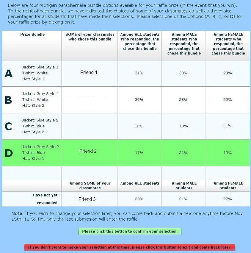
                                              Figure 1
                                Webpage for Sports Paraphernalia Raffle

         To collect social network information, we first ask the participants to nominate ten

students in the class with whom they have interacted most frequently.8 To ensure privacy,9 we

8
  To facilitate the nomination process, our JAVA program has a built-in search tool. Participants can easily locate
the nominees’ names by typing part of their first or last names. The search tool helps us avoid typos and solves the
problem that participants may not necessarily remember the full name of all the nominees.
9
  This procedure was included upon the request from the Institutional Review Boards of Health Sciences and
Behavioral Sciences (IRB-HSBS).

                                                                                                                   22

later provide the participants with an option to indicate to which nominees they are unwilling to

disclose their choice information. We then invite the participants to enter the two raffles. We

finally collect demographic information including gender, time spent on email daily, confidence

in apparel taste, knowledge about cell phone headset, and interest in winning the products.

In the post-influence stage, we first launch the online raffle for sports paraphernalia. All

participants receive an email that includes the URL that directs them to a webpage. On the page,

they can select one of four sports paraphernalia bundles they wish to receive should they win the

raffle. The four prize options are described by the same attributes as those used in the pre-

influence stage (Figure 1).10 The four options are relatively close to one another with regard to

their overall utilities (computed from the part-worth estimates obtained from the pre-influence

stage) and pre-tested with a similar pool of participants to have similar choice shares.

To facilitate choice interdependence, we show the participants the choices that were

previously made by their “friends.”11 One’s friends are other participants who specify him or her

as someone they have interacted with frequently and agree to share choice information with in

the pre-influence stage. For sports paraphernalia, we expect that the participants’ product

decisions may also be influenced by a larger-scale social interaction based on gender (i.e. gender

norm) (Brock and Durlauf 2001; Miller and Prentice 1996). To examine whether the influence of

gender norm can co-exist with the social influence at the reference group level (i.e., global vs.

local social interactions), we show each participant the aggregate proportions of other

participants choosing each option. The aggregate proportions are computed based on: 1) all

participants who have already chosen each option; 2) only female participants who have already

10
We omit price, as including price may have prompted students to choose the most expensive bundle.
11
To further induce social interactions, the experiment features the real-time delivery of friends’ choices during the
raffle period. The procedure works as follows. The first time a participant makes a choice or every time he or she
changes a choice, emails are sent out to his or her “friends.” The email informs each participant’s friends about his
or her most recent activity, and urges the friends to visit the raffle page. The webpage URL is included in the email.

chosen each option; and 3) only male participants who have already chosen each option at a

particular time point. The participants can change their prize choice as often as they wish before

the end of the raffle. We inform them that if they do not make a choice, one of the four bundles

will be drawn randomly as their prize should they win the raffle. Our database is updated in real-

time to assure that the webpage offers up-to-date information about the friends’ activities. To

increase the response rate, we send an email reminder in the middle of the raffle.

A week after we launch the second raffle for the Bluetooth headset. The setup is very

similar to the paraphernalia raffle, except that participants do not see the aggregate proportions

of male and females who are choosing each Bluetooth option. We do not expect a gender norm

to be relevant for this product category. In addition, the default option for the participants who do

not make a prize choice is a wired headset priced at $29 (the outside option we use in the

conjoint experiment in the pre-influence stage). The raffle is closed after a week. Two email

reminders are sent out during this period. A winner is drawn for each raffle at the conclusion of

the study.

EMPIRICAL ANALYSIS

Descriptive Statistics of Participants and Their Social Network

Participant Profile. There are 292 participants in the pre-influence stage, among which

215 agree to participate in the raffles in the post-influence stage. The general demographic

profiles of the participants who agree to enter the raffles and those who do not are not

significantly different, except that those in the raffles are more interested in the products they can

win (Table 1). All the analysis discussed below is based on these 215 participants.

Among the 215 raffle participants, 21.4% rate their confidence in apparel taste greater

than 6 on a 1-7 scale, 1 being least confident), and 18.6% rate their level of knowledge about cell

phone headsets greater than 5 on a 1-7 scale, 1 being not knowledgeable. More than half of the

participants are “very interested” in winning a sports paraphernalia bundle, with a rating of 7 on

a 1-7 scale (1 being “not interested all at”), and the mean rating is 5.99. For the Bluetooth

headset, interests are more evenly distributed, although one-third of the ratings are 7, and the

mean rating is 4.51 (on a 1-7 scale).

                                                   Table 1
                                             Descriptive Statistics

Variables                   Participants’ mean              Non-participants’            Test statistic1
                            (Std. Dev.)                     mean (Std. Dev.)                  (df)
Gender                           60.9% male                   63.6% male                    .08 (1)
Apparel confidence                5.52 (1.18)                 5.51 (1.30)                  .09 (123)
Headset knowledge                 3.59 (1.75)                 3.27 (1.70)                 1.38 (138)
Time spent on email                 38.6% 2                     28.6%                       5.43 (3)
Interest in sports                5.99 (1.34)                 3.22 (2.06)                10.05 (78)**
paraphernalia
Interest in Bluetooth              4.51 (2.12)                  2.35 (1.77)              8.11 (119) **
headset
1
  Chi-square test is used for gender and time spent on email. Independent-sample t-test is used for the remaining
variables.
2
  Percentage of participants spending more than an hour on email every day.
**
   Two sided p-value is < .05,

         Social Network Profile. Figure 2 depicts the directed social network among the raffle

participants. Each node represents a participant. Recall that in our experiment, one’s friends are

defined as participants who nominate him or her as one of those with whom they have frequently

interacted and agree to share choice information. In other words, a participant cannot choose his

or her friends. It is other participants who nominate themselves to be his or her friends. An arrow

indicates the direction of the nomination. For instance, an arrow from node 110 to 2 means

participant 110 nominates participant 2, and becomes one of participant 2’s friend. A double-

                                                                                                                    25

headed arrow between 185 and 196 means both participants nominate each other. Among the

628 pairs of connected participants (the same two individuals are only counted as one pair),

26.6% of them have arrows both in and out (i.e., have reciprocal connections).

                                             Figure 2
                                       Social Network Plot

       It is not surprising that a small group of participants in the network are substantially more

popular (i.e., many other students nominate each of them as one of their “friends”) than the rest.

We use the size of each node to represent the number of friends each participant has. The bigger

the node, the larger the number of friends he or she has (i.e., more arrows in). Participants 9, 110,

and 140 are examples of the popular participants. On the flip side, we use color to denote the

number of others each participant nominates. The three orange nodes, 24, 50, and 121, each

nominates nine students (nine arrows out) though they themselves do not get as many

nominations from others (i.e., fewer arrows in). From this plot, we do not see a strong correlation

between popularity (being nominated) and the number of nominations. Nodes of the same size

                                                                                                  26

can thus have a variety of colors.

                                                         Table 2
                                                Network Structure Statistics

               Effects                                           Network Statistics                  Values
 Mean in/out degree                                      e /n
                                               1 i , j  n ij                                        3.7
 Variance of in degree                      var( 1 j  n e ji )                                     7.0
 (prestige)
 Variance of out degree                     var( 1 j  n eij )                                      6.0
 Percentage of isolates (no                # ( 1 j  n e ji  1 j  n eij  0) / n               2.3%
 arrow in or out)
 Percentage of arrow out only              # ( 1 j  n e ji  0, 1 j  n eij  0) / n            4.2%
 Percentage of arrow in only               # ( 1 j  n e ji  0, 1 j  n eij  0) / n            12.6%
 Density                                                 e / n ( n  1)
                                               1 i , j  n ij                                       1.7%
 Percentage of reciprocal
 connections
                                           
                                       1 i  j  n
                                                        2eij e ji / n ( n  1)                       .73%
 Percentage of transitive
 triads
                                                                      e e e / n ( n  1)( n  2 )
                                       1 i , j , i '  n , i  j  i ' ij ji ' ii '                 .007%
eij = 1 if i nominates j, 0 otherwise.

          The network solicitation procedure leads to participants having 3.7 friends on average.

The most popular participants have 12 friends, while 14 participants have no friends. Table 2

provides some network structure statistics. As expected, the density, reciprocity, and transitivity

are low as we work with a relatively large network. Two characteristics of our experimental

setup also contribute to the network’s sparse nature. First, we ask each participant to select up to

ten friends with whom they have interacted most frequently for a practical reason. Narayan, Rao,

and Saunders (2011) allow participant to nominate up to N-1 (the N sample size = 70) others as

their influencers. This would have been a timely prohibited task for us with 292 participants, plus

we propose a design that is applicable for a large network. Other researchers take a similar

approach restricting the number of nominations per participant (Lieder et al. 2009; Nair,

Manchanda, and Bhatia 2010). Second, as participants’ choices are shared along with their

                                                                                                              27

names, to protect privacy participants are given the right to opt out from sharing choice

information with the friends they nominate, which makes our network even sparser. Unlike in

Centola (2010, 2011) where people do not know each other prior to the experiment and their

information is shared with the screen names they choose, which eliminates the privacy issue, our

experiment hinges upon actual friendship and cannot get around the privacy issue. Privacy is also

not a concern in a field experiment, where focal behavior is naturally expected to be observed

among peers (Aral and Walker 2011, 2012).

In Table 2, 4.2% of the participants receive no nomination from other students, although

they nominate at least one other student as their friend (i.e., arrow out only). We observe that

85.1% of the participants share choices with at least one friend, and 93.5% of the participants can

observe at least one other participant’s choice. At the same time, 14.9% (% arrow in only plus %

isolate) are not willing to nominate anybody with whom they will eventually share their choice

information. The major difference between them and those sharing choice information is that

they are more socially peripheral, i.e., they have fewer friends sharing choice information with

them (on average 2.4 vs. 3.9 friends). There is no significant difference in other demographic

profiles, except that participants not sharing on average are less knowledgeable about a cell

phone headset (3.1 vs. 3.7 on a 1-7 point scale).

Raffle Choice Summary. For sports paraphernalia, 167 participants visit the webpage, and

62.3% of them are male, which is similar to the proportion of males among the 215 raffle

participants. Among the 25 participants who visit the page multiple times, 17 do not change their

choices in all the visits, whereas the remaining eight first did not choose any option but then pick

an option later. The percentages of people choosing options 1 to 4 and not choosing any of the

options are 30.5%, 38.9%, 9.0%, 16.8%, and 4.8%, respectively.

For the Bluetooth headset, 97 participants visit the webpage, and 25.8% claim to be

knowledgeable (rating their knowledge greater than 5 on a 1-7 scale), which is higher than the

percentage among the 215 enrolled (18.6%). The main reason could be that the participants who

consider themselves knowledgeable are more interested in winning a Bluetooth headset than

those who are less knowledgeable, as the mean winning interest are 5.9 and 4.2 for the more

knowledgeable and less knowledgeable group, respectively. Among the 97 participants, 92 also

log on to the paraphernalia raffle page. Thirty-four participants visit the page multiple times, and

28 of them maintain the same choices in all the visits. The remaining 6 first did not choose an

option but later choose one. The percentages of people choosing options one to four and not

choosing any of the options are 14.4%, 3.1%, 74.2%, 2.1%, and 6.2%, respectively.12

Analysis of Participants’ Initial Preferences

         We use the hierarchical Bayes logit model (Allenby and Rossi 1999) to fit the conjoint

                                                                                               P
choice data from the pre-influence stage. Participant i’s utility of option k is              
                                                                                               p 1
                                                                                                       I I
                                                                                                        x
                                                                                                      ip ipq ,k     ikI ,

where  ipI captures individual i’s initial preference for the p-th product attribute, x ipq
                                                                                          I
                                                                                             , k indicates

the p-th attribute’s value for option k in task q,  ikI is an error term following type I extreme

value distribution, and the superscript I denotes initial preference. All the attributes are dummy-

coded including price. The model specifications for the sports paraphernalia and the Bluetooth

headset are the same except that for the headset, the participants also have an option to choose an

ear-plug version at $29. Hence, we estimate the preference (  i0I ) for this outside option for the

12
   Option 1: Motorola, black, 13 grams, 8-hr talk time, no noise cancellation; Option 2: Motorola, silver, 8 grams, 5-
hr talk time, no noise cancellation; Option 3: Plantronics, silver, 13 grams, 8-hr talk time, noise cancellation; Option
4: Plantronics, black, 8 grams, 8-hr talk time, no noise cancellation).

                                                                                                                              29

You can also read