A protocol for dynamic model calibration
←
→
Page content transcription
If your browser does not render page correctly, please read the page content below
A protocol for dynamic model calibration
                                            Alejandro F. Villaverde 1 , Dilan Pathirana 2 , Fabian Fröhlich 3,4,5 , Jan Hasenauer 2,3,4,∗ and Julio R. Banga 6,∗
arXiv:2105.12008v2 [q-bio.QM] 26 May 2021

                                                  1
                                                      Universidade de Vigo, Department of Systems Engineering & Control, Vigo 36310, Galicia, Spain
                                                           2
                                                               Faculty of Mathematics and Natural Sciences, University of Bonn, Bonn 53115, Germany
                                                  3
                                                      Institute of Computational Biology, Helmholtz Zentrum München, Neuherberg 85764, Germany
                                                                4
                                                                    Center for Mathematics, Technische Universität München, Garching 85748, Germany
                                                                                    5
                                                                                        Harvard Medical School, Cambridge, MA 02115, USA
                                                                          6
                                                                              Bioprocess Engineering Group, IIM-CSIC, Vigo 36208, Galicia, Spain
                                                       ∗
                                                           To whom correspondence should be addressed: jan.hasenauer@uni-bonn.de, j.r.banga@csic.es.

                                                                                                          Abstract
                                                     Ordinary differential equation models are nowadays widely used for the mechanistic description of
                                                 biological processes and their temporal evolution. These models typically have many unknown and
                                                 non-measurable parameters, which have to be determined by fitting the model to experimental data.
                                                 In order to perform this task, known as parameter estimation or model calibration, the modeller faces
                                                 challenges such as poor parameter identifiability, lack of sufficiently informative experimental data,
                                                 and the existence of local minima in the objective function landscape. These issues tend to worsen
                                                 with larger model sizes, increasing the computational complexity and the number of unknown param-
                                                 eters. An incorrectly calibrated model is problematic because it may result in inaccurate predictions
                                                 and misleading conclusions. For non-expert users, there are a large number of potential pitfalls. Here,
                                                 we provide a protocol that guides the user through all the steps involved in the calibration of dynamic
                                                 models. We illustrate the methodology with two models, and provide all the code required to repro-
                                                 duce the results and perform the same analysis on new models. Our protocol provides practitioners
                                                 and researchers in biological modelling with a one-stop guide that is at the same time compact and
                                                 sufficiently comprehensive to cover all aspects of the problem.
                                                 Key words: systems biology; dynamic modelling; parameter estimation; identification; identifiabil-
                                                 ity; optimisation.

                                                 Introduction
                                                 The use of dynamic models has become common practice in the life sciences. Mathematical modeling
                                                 provides a rigorous, compact way of encapsulating the available knowledge about a biological process.
                                                 Perhaps more importantly, it is also a tool for understanding, analysing, and predicting the behaviour
                                                 of a complex system under conditions for which no experimental data are available. To these ends,
                                                 it is particularly important that the model has been developed with that specific purpose in mind.
                                                      In biomedicine, dynamic models are used for basic research as well as for medical applications.
                                                 On one hand, dynamic models facilitate an understanding of biological processes, e.g. by identifying
                                                 from a list of alternative mechanisms the most plausible one [50]. On the other hand, dynamic models
                                                 with sufficient mechanistic detail can be used to make predictions, including the selection of drug
                                                 targets [67], and the outcome of individual and combination treatments [25, 36]. In bio- and process
                                                 engineering, dynamic models are used to design and optimise biotechnological processes. Here, models

                                                                                                              1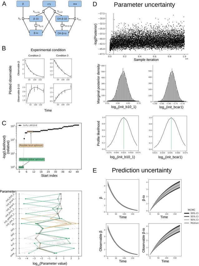
are, for instance, used to find the genetic and regulatory modifications that enhance the production of
a target metabolite while enforcing constraints on certain metabolite levels [1, 9, 74, 91]. In synthetic
biology, dynamic models guide the design of artificial biological circuits where fine-tuned expression
levels are necessary to ensure the correct functioning of regulatory elements [39, 45, 76, 82]. Beyond
these topics, there is a broad spectrum of additional research areas.
    The choice of model type and complexity depends on which biological question(s) it should address.
Once this has been decided, the relevant biological knowledge is collected, e.g. from databases such
as KEGG [44], STRING [80], and REACTOME [21], or from the literature. Furthermore, already
available models can be used, e.g. from JWS Online [61] or Biomodels [51], and information about
kinetic parameters might be extracted, e.g. from BRENDA [13] or Sabio-RK [102]. This information
is used to determine the biological species and biochemical reactions that are relevant to the process.
In combination with assumptions about reaction kinetics – e.g. mass action or Michaelis-Menten
– these elements allow the construction of a tailored mathematical model, which will usually have
nonlinear dynamics and uncertainties associated to its structure and parameter values [86]. The
model can be specified in a standard format such as SBML, to take advantage of the ecosystem of
tools that already support standard format [40].
    The advent of high-throughput experimental techniques and the ever-growing availability of com-
putational resources have led to the development of increasingly larger models. Common models
possess tens of state variables and tens to a few hundreds of parameters (see [34, 93]). Large mod-
els can even possess thousands of state variables and parameters [25]. Dynamic models need to be
calibrated, i.e. their unknown parameters have to be estimated from experimental data. In model
calibration, the mismatch between simulated model output and experimental data is minimised to
find the best parameter values [2,28,29,42,64]. Model calibration is a process composed of a sequence
of steps, which usually need to be iterated [5] until a satisfactory result is found. It may be seen
as part of a more general problem sometimes called reverse engineering [90] or (nonlinear) systems
identification [70].
    In this work, we consider the calibration of ordinary differential equation (ODE) models. ODE
models are widely used to describe biological processes, and their calibration has been discussed
in protocols for different classes of processes, including gene regulatory circuits [71], signalling net-
works [29], biocatalytic reactions [20], wastewater treatment [57, 103], food processing [88], biomolec-
ular systems [85], and cardiac electrophysiology models [100]. Yet, these protocols focus on individual
aspects of the calibration process (relevant for the sub-discipline) and/or lack illustration examples
and codes that can be reused. The papers [57] and [103] focus on parameter subset selection via
sensitivity and correlation analysis, and on subsequent model optimisation. The works of [71], [88]
and [20] consider only low-dimensional models and do not provide in-depth discussion of scalability.
The paper [29] neither covers structural identifiability analysis nor experimental design, and describes
a prediction uncertainty approach with limited applicability. The works of [85], [100] and [20] dis-
cuss most aspects of the calibration process, but do not provide a step-by-step illustration with an
example model and codes. The work of [77] is tailored to users of the MATLAB software toolbox
Data2Dynamics [65].
    This protocol aims to provide a comprehensive description of the steps of the calibration process,
which integrates recent advances. An outline of the procedure is depicted in Figure 1. The article is
structured as follows. First we describe the requirements for running the calibration protocol. Then,
we describe the individual steps of the protocol. The theoretical background for each step, along with
a brief review of available methodologies, is provided in boxes. After some troubleshooting advice, we
illustrate the application of the protocol for two case studies. For the sake of clarity, only a concise
summary of the application results is reported in the main text of this manuscript; complete details
are given in the supplementary information. To ensure the reproducibility of the results, we provide
computational implementations used for the application of the protocol steps to the case studies in
the form of MATLAB live scripts, Dockerfiles, and Python-based Jupyter notebooks.

                                                   2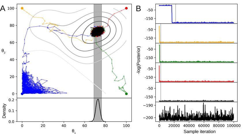
START                                                                                                                            Choose:
                                                                                                                                            Criterion,
                                                                                                                                             method
                                                                                                                                             Obtain:
                                                                                                                                           Best model
       Model equations
       (with unknown      Experimental data
                                                                                                                                           (OPTIONAL)
        parameters)                                                                                Choose:
                                                                                 (OPTIONAL)                                                  Model
                                                                                                   Optimality criterion, optimisation       selection
                                                                                  Optimal          method, experimental constraints
                                                                                 experiment        Obtain:
                                                                                   design
                                                                                                   New experimental setup
            in                 in

             1                 2                   3                 4                 5                          6                     Calibrated
                         Formulation of                                                                       Prediction
         Structural                            Parameter         Goodness          Practical
       identifiability      objective         optimisation         of fit        identifiability
                                                                                                             uncertainty
                                                                                                            quantification
                                                                                                                                  out     model
        (SI) analysis       function                                                analysis
          Choose:          Choose:              Choose:
                                              Optimisation
                                                                 Choose:
                                                               Criterion for
                                                                                   Choose:                    Choose:                     (END)
      SI method (and        Type of                                               Uncertainty                Uncertainty
      possibly refor-      objective           method,       assessing the fit   quantification             quantification
        mulation, if       function             options                            method                     method
      unidentifiable)

          Obtain:           Obtain:             Obtain:           Obtain:           Obtain:                     Obtain:
      A fully SI model     Objective           Parameter      Goodness of fit,    Confidence                  Confidence
                           function            estimates,         possibly        intervals of                intervals of
                                                model fit       invalidated       parameters                  predictions

         Figure 1: Block diagram of the model calibration process presented in this protocol.

Materials
This section describes the inputs and equipment required to run the protocol.

Hardware: a standard personal computer, or a computer cluster. For demonstrating the applica-
tion of the protocol, in the present work we have performed Step 1 on a standard laptop with a 2.40
GHz processor and 8 GB RAM. Optimisation, likelihood profiling, and sampling were performed on
a laptop with an Intel Core i7-10610U CPU (eight 1.80GHz cores) and 32 GB RAM, with a total
runtime of up to 2 days, per model.

Software: a software environment with numerical computation and visualisation capabilities, along
with specialised toolboxes that facilitate performing specific protocol steps. Table 1 lists the software
resources used in this work.

Model: a dynamic model described by nonlinear ODEs of the following form:
                                                  ẋ = f (x, θ, t) , x(t0 ) = x0 (θ),
                                                                                                                                                         (1)
                                                  y = g(x, θ, t),

in which x(t) ∈ Rnx is the state vector at time t with initial conditions x0 (θ), y(t) ∈ Rny is the
output (i.e. observables) vector at time t, f and g are possibly nonlinear functions, and θ ∈ Rnθ is
the vector of unknown parameters.
   In this work we used a carotenoid pathway in Arabidopsis thaliana [11], and an EGF-dependent
Akt pathway of the PC12 cell line [27], taken from the PEtab benchmark collection [34] available
at https://github.com/Benchmarking-Initiative/Benchmark-Models-PEtab. An illustration of both
models is provided in panels A of Fig. 5 and Fig. 6.

Data: a set of time-resolved measurements of the model outputs. In the present work, data was
taken from the aforementioned PEtab benchmark collection.

                                                                      3
Name Type Steps Reference Website Environment
MATLAB environment all http://www.mathworks.com
Python environment all https://www.python.org
SBML model format input [40] http://www.sbml.org MATLAB, Python
PEtab data format input [69] https://github.com/PEtab-dev/PEtab Python
STRIKE-GOLDD tool (SI analysis) 1 [95] https://github.com/afvillaverde/strike-goldd MATLAB
AMICI tool (simulation) 2 [24] https://github.com/AMICI-dev/AMICI Python
pyPESTO tool (various steps) 3, 5, 6 [68, 75] https://github.com/ICB-DCM/pyPESTO Python
Fides tool (param. optimisation) 3, 5 [23] https://github.com/fides-dev/fides Python
SciPy tool (various steps) 3, 5 [96] https://www.scipy.org Python
Data2Dynamics tool (various steps) 3, 5, 6, (O) [65] http://www.data2dynamics.org MATLAB
Table 1: Software resources for dynamic model calibration used in this work.
Procedure
The protocol consists of six main steps, numbered 1–6, which consist of sub-steps. Furthermore,
we describe two optional steps. The workflow is depicted in Fig. 1 and described in the following
paragraphs.
STEP 1: Structural identifiability analysis
Structural identifiability is analysed to assess whether the values of all unknown parameters can be
determined from perfect continuous-time and noise-free measurements of the observables under the
given set of experimental conditions [17, 99]. Structural non-identifiabilities imply that there are
several model parameterizations, e.g. due to symmetries or redundancies in the model structure,
which yield exactly the same observables. An overview of the available methodologies for structural
identifiability analysis is provided in Box 1. Fig. 2 illustrates possible sources of structural non-
identifiability and the related issues. The structural identifiability analysis can be complemented
by observability analysis, which determines if the trajectory of the model state can be uniquely
determined from the observables.
The first step in the protocol is thus:
STEP 1.1
Analyse the structural identifiability of the model with one of the methods described in Box 1.
If all parameters are structurally identifiable and all state variables are observable, we continue
with Step 2.1. Otherwise, we recommend to determine the source of the structural non-identifiability
as an intermediate step (1.2). Ideally, the parametric form of the non-identifiable manifold (i.e. the
set of parameters that yield identical observables) is determined. Some tools offer this functionality
or at least provide hints.
STEP 1.2
If parameters are structurally non-identifiable or state variables unobservable, use knowledge about
the structure of the non-identifiable manifold to
• reformulate the model by merging the non-identifiable parameters into identifiable combinations,
OR
• fix the non-identifiable parameters to reasonable values.
4Figure 2: Structural identifiability analysis. (A) Diagram of a simplified model of mRNA translation
considering only the process in the cytosol. The model captures the translation of mRNA and the degradation
of mRNA and protein. (B) Mathematical formulation (ODEs) of mRNA translation dynamics [3] involving two
states, mRNA and GFP. (C) The model output is the fluorescence intensity, which is proportional to the GFP
level. The model has five unknown parameters: the initial condition of the unmeasured state (mRNA0 ), three
kinetic parameters (γ, δ, k), and an output scaling parameter (s). Given its simplicity, it is possible to calculate
the output time-course analytically (here shown for γ 6= δ). The resulting function contains the product of
three parameters (s · k · mRN A0 ), which is shown in orange, and an expression involving δ and γ, which are
shown in green. The latter expression is symmetrical with respect to δ and γ: their values can be exchanged
without changing the result. Thus, these two parameters are not structurally globally identifiable, but only locally
identifiable with two possible solutions. Furthermore, the product (s · k · mRN A0 ) allows for an infinite number
of parameter combinations; the three involved parameters are structurally non-identifiable. (D) Illustration of
structural non-identifiability: the time-course of the model output is identical for an infinite number of parameter
vectors. (E) Illustration of unobservability caused by non-identifiability. For illustration purposes, three different
parameter vectors are shown, all of which produce the same model output. Each of them yields a different
simulation of the mRNA time-course; thus, this state cannot be determined. (F) Illustration of the correlations
between the non-identifiable parameters. The line indicates parameter combinations for which the time-dependent
output is identical.
In both cases, the information about the non-identifiability needs to be retained to later perform a
proper analysis of the prediction uncertainties. If this point is not taken into account, the obtained
results are only valid for the reformulated model, but not for the original one – a fact that is often
disregarded.
An alternative to the reformulation of the model or the fixing of parameters is to plan additional
experiments, if possible. These can be experiments with new experimental conditions, new observ-
ables, or both (keeping experimental constraints in mind). The additional information should be
recorded such that more, ideally all, parameters are structurally identifiable.
5Box 1. Methods for STEP 1: Structural identifiability analysis
Structural identifiability (SI) can be analysed using a broad spectrum of methods exploiting, e.g., Taylor
and generating series, differential algebra, differential geometry, and probabilistic numerics [15, 59, 89]. In
essence, these methods aim to assess whether the mapping from parameters to observables is invertible
for almost all points in parameter space.
When choosing a method, the trade-off between generality and applicability must be taken into ac-
count. Most available methods are tailored to rational models, i.e. f and g can be expressed as fractions
of polynomials. Structural local identifiability of rational models can be assessed efficiently using e.g. the
exact arithmetic rank method in [46,72]. Structural global identifiability analysis requires more computa-
tionally expensive techniques that do not scale well, hence, this approach can only be applied to models
with tens of parameters and state variables. For non-rational models, a higher-dimensional polynomial
or rational model can be formulated with an identical input-output map [60]. This immersion shifts the
non-rational relations from the vector field to constraints on the initial conditions. These constraints
can be relaxed to apply methods for rational models; however, for the relaxed problem, results about
non-identifiability may not be conclusive [14].
In the present work we used STRIKE-GOLDD to assess structural local identifiability and observability
[95]. Tools for structural global identifiability analysis include GenSSI2 [54], SIAN [37], COMBOS [58],
and DAISY [66].
STEP 2: Formulation of objective function
The objective function measuring the mismatch of simulated model observables and measurement
data is defined. The choice of the objective function depends on the characteristics of the measurement
technique and accounts for knowledge about its accuracy. Possible choices are discussed in Box 2.
STEP 2.1
Construct an objective function.
STEP 3: Parameter optimisation
Parameter estimates are obtained by minimising the objective function. To this end, numerical
optimisation methods suited for nonlinear problems with local minima should be employed. Available
methodologies and practical tips for their application are discussed in Box 3, and key aspects are
illustrated in Fig. 3.
STEP 3.1
Launch multiple runs of local, global, or hybrid optimisation algorithms. The number of runs required
is model-dependent. For an initial optimisation we recommend at least 50 runs with purely local
searches, or at least 10 runs with global or hybrid searches.
Accurate gradient computation is required for gradient-based optimisation. Before optimisation,
check that the gradients appear correct by evaluating the gradient at a point, and then compare
this with forward, backward, and central finite difference approximations of the gradient that are
evaluated with different step sizes. Such a gradient check is a common, possibly optional, feature of
tools that provide gradient-based optimisation.
6Box 2. Theory for STEP 2: Formulation of objective function
The objective function encodes the characteristics of the measurement process and potential prior knowl-
edge. It can be composed of up to two parts:
• the likelihood function p(D|θ) provides the likelihood of measuring the dataset D given the model
parameters θ, and
• the prior distribution p(θ) encodes additional belief.
Frequentist approaches only use the likelihood function, and the common choice of the objective func-
tion is the negative log-likelihood function, J(θ) = − log p(D|θ). Bayesian approaches use the posterior
instead of only the likelihood, hence also consider the prior distribution, yielding the unnormalised nega-
tive log-posterior J(θ) = − log p(D|θ) − log p(θ) (which disregards the marginal probability). In contrast
to the likelihood function and the posterior distribution, the logarithmic transformations are numerically
easier to evaluate and allow for faster optimiser convergence [34].
Under the assumption of independent measurements and normally distributed noise, the negative log-
likelihood function is
ny nt " #
yj (tk ) − yj (tk , θ) 2
m
1 XX 2
J(θ) = log 2πσj (tk ) + , (2)
2 j=1 σj (tk )
k=1
in which yjm (tk )
is the measured value and yj (tk , θ) is the simulation result of the j-th observable, at time
point tk . The corresponding standard deviation of the measurement noise is denoted by σj (tk ), and can be
known (e.g. determined from multiple measurement replicates) or a function of the parameters. a In the
case of known standard deviations, the summands log(2πσj2 (tk )) are independent of the parameter vector,
and can be disregarded for parameter optimisation and uncertainty analysis. This yields the weighted
least squares objective function:
ny nt
X X 2
J(θ) = wj (tk ) yjm (tk ) − yj (tk , θ) (3)
j=1 k=1
with wj (tk ) = σj−2 (tk ). Sometimes this objective function is also applied without proper statistical
motivation, e.g. without linking the weights to the noise levels, which does not yield a proper frequentist
formulation of the calibration problem.
The likelihood function is based on the assumed or observed probability distribution of the experimen-
tal error. Normal and log-normal distributions are common choices [35], but in a recent study Laplace
distributions have also been used to achieve robustness against outliers [56]. For count measurement,
distributions such as the binomial and negative binomial distributions appear to be suited. Furthermore,
the consideration of the correlation of measurement errors might be necessary. An alternative to statisti-
cally motivated prior distributions p(θ) are more mathematically motivated regularisation functions. In
general, regularisation is used to tackle the problem that models are often over-parameterised. In this
case, the calibration problem is ill-posed and small perturbations in the data can result in very different
parameter estimates [31]. Regularisation techniques address this problem by penalizing undesirable pa-
rameter choices. Tikhonov regularisation penalises large parameter values, and pushes estimates towards
zero. Mathematically, it is identical to a normally distributed prior p(θ) with mean zero. Alternative
regularisation schemes include [55] parameter subset estimation, truncated singular value decomposition,
principal component analysis, and Bregman regularisation.
The objective functions encountered in model calibration are mostly nonlinear and non-convex, and
possess multiple optima. Furthermore, there are frequently flat regions (in particular in the presence of
non-identifiabilities), and rims (e.g. at bifurcation points).
a In many applications the measurements are repeated to obtain biological or at least technical replicates. In
this case, one can either (i) use all replicates as measurements and set the noise level to the standard deviation,
or (ii) use the mean of the replicates as measurement and set the noise level to the standard error of mean. A
combination of (i) and (ii) is statistically not meaningful.
7Figure 3: Parameter optimisation. (A) Multi-start local optimisation involves many local optimisations that
are distributed within the parameter space. In systems with multiple optima, many starts may be required to find
the global optimum. Trajectories are indicated by arrows, with their initial points indicated with “×”. The contour
plot shows the negative log-likelihood, with darker contours indicating lesser (better) values. In all subfigures, the
colours pink (global) and brown (local) are used to indicate results that correspond to a particular optimum, and
parameters are labelled as θ with an index as the subscript. This subfigure is for illustration purposes only, as it
is generally infeasible to produce. (B) Convergence of starts towards an optimum can be assessed with a waterfall
plot, where the existence of (multiple) plateaus indicates optimiser convergence. If plateau(s) are not seen, possible
solutions include: additional starts; alternative initial points; or alternative global optimisation methods. (C) A
parallel coordinates plot can be used to assess whether parameters are well-determined. Here, lines belonging to
a single optimum overlap, indicating that the parameters that have converged to the corresponding optimum are
well-determined.
STEP 3.2
Evaluate the reproducibility of the fitting results by comparing the optimal objective function values
achieved by different runs. The optimal objective function values should be robustly reproducible,
meaning that a substantial number of runs (rule-of-thumb: 5) should find it. If this is not the
case, repeat Step 3.1 with a larger number of runs. Note that the difference between runs that is
considered negligible should be statistically motivated. For the use of log-likelihood and log-posterior
this corresponds to an absolute difference, not a relative one [34].
STEP 4: Goodness of fit
The quality of the fitted model should be assessed by visual inspection. It is also possible to use
quantitative metrics for this purpose. Details are provided in Box 4.
8Box 3. Methods for STEP 3: Parameter optimisation.
Objective functions encountered in systems biology are usually non-convex and multi-modal. Hence,
global optimisation methods are required to robustly determine the optimal solution. Common choices
are (i) a multi-start strategy that performs local searches from different starting points [64], and (ii) a
hybrid methodology combining a metaheuristic algorithm with local searches [93]. Independently of the
employed method, it is advisable to run the optimisation method several times [38].
Independently of the setting (multi-start or hybrid) in which the local searches are performed, it is
recommended to use a gradient-based local method, which exploits the knowledge about the gradient of
the objective function to drive the search [93]. Gradient computation using adjoint sensitivities has been
shown to outperform forward sensitivities and finite differences for medium- and large-scale models [24].
Finite differences are least reliable, as an appropriate choice of the step-size is problematic and depends
on the parameters. Furthermore, for most parameters it is beneficial to estimate them on a logarithmic
scale [34, 47, 64].
Many optimisation methods can exploit parallel infrastructure, allowing for a reduction in computation
times if a multi-core computer or cluster is available [62, 65].
Box 4. Methods for STEP 4: Assessment of the goodness of fit.
The root-mean-square error (RMSE) between simulated and measured observables, i.e. the square root of
the mean squared error, provides a quantitative metric of the goodness of fit. The normalised root mean
squared error (NRMSE) is obtained by dividing the RMSE by the range of the measurements, and it is
usually more useful since it enables a direct comparison between different observables and/or estimation
methods. The NRMSE has the additional advantage of being independent of the noise in measurements
and the number of data points used for the fitting. These and other metrics are further discussed in [52].
Complementary to this, the achieved objective function value can be compared with the expected
objective function value. The distribution of expected objective function values for the data generating
model with the true parameters can be constructed from the knowledge of the model and the measurement
setup. For normally distributed measurement noise with known standard deviation, the sum of squared
residuals follows a chi-squared distribution with nD (number of data points) degrees of freedom. However,
while the distribution for the true parameter is analytically tractable, for the estimated parameter this
is not the case. To assess whether the achieved objective function value is plausible, approximations can
be employed. For linear regression problems it is known that the sum of squared residuals at the optimal
parameters follows a chi-squared distribution with nD − nθ degrees of freedom, where nθ is the number of
estimated parameters. This is often also used as an approximation for ODE models [29], but for certain
models (e.g. those with oscillatory dynamics) this can be off. An alternative is the use of bootstrapping
procedures, in which a problem-specific distribution is constructed [19].
If the achieved objective function value is much larger than most values expected under the distribution,
this can indicate underfitting. This implies that either the optimisation was not successful or that the
model is inappropriate. If the achieved objective function value is much smaller than expected, this is a
sign of overfitting, meaning that not only the signal in the measurement data but the noise is described.
Under- and overfitting are possible causes of wrong model predictions and should be avoided.
A way of controlling for overfitting is to perform cross-validation. To this end, a subset of the data
must be left out of the optimisation in STEP 3. Afterwards, the calibrated model is used for predicting
this data subset. Overfitting appears if the model achieves a good fit in the optimisation, but then fails
to generalise to observables or experimental conditions that it was not trained with.
9STEP 4.1
Assess the goodness of the fit achieved by the parameter optimisation procedure.
If the fit is not good, further action is required. Proceed to STEP 4.2.
STEP 4.2
If the fit is not good enough, check convergence of the optimisation methods.
1. If there are hints that searches were stopped prematurely (e.g. error messages that indicate
that local optimisations did not converge), go back to STEP 3: modify the settings of the
optimisation algorithms (e.g. increase maximum allowed time and/or number of evaluations)
and run the optimisations again.
2. If there are no signs of a premature stop, the problem may be that the optimal solution lies
outside the initially chosen parameter bounds → go back to STEP 3: set larger parameter
bounds and run the optimisations again.
3. If the actions above do not solve the issue, it may be because the optimisation method is not
well suited for the problem → go back to STEP 3: choose a different method and run the
optimisations again.
If the new optimisations performed in STEP 4.2 do not yet yield a good fit, there may be a
problem with the choice of objective function. Proceed to STEP 4.3.
STEP 4.3
If the fit is not good enough, go back to STEP 2 and select a different objective function.
If the new optimisation results are still inappropriate, the problem might be the model structure.
Proceed to STEP 4.4.
STEP 4.4
If the fit is not good enough, go back to the model equations and perform a model refinement.
STEP 5: Practical identifiability analysis
The task of quantifying the uncertainty in parameter estimates is known as practical (or numerical)
identifiability analysis. It involves calculating univariate confidence intervals or multivariate confi-
dence regions for the parameter values. Key concepts and tools for practical identifiability analysis
are listed in Box 5. Practical identifiability issues are illustrated in Figures 5D and 6D.
STEP 5.1
Perform practical identifiability analysis with one of the methods described in Box 5. If large uncer-
tainties in parameter estimates are revealed, then proceed to STEP 5.2.
STEP 5.2
If there are large uncertainties, then:
1. If it is possible to perform new experiments → add more experimental data. In this case, the
experiment should be optimally designed in order to yield maximally informative data. This is
described in the following section.
10Box 5. Methods for STEP 5: Practical identifiability analysis
The Fisher information matrix (FIM) is a widely used measure of the information content of the experi-
mental data that provides information about the practical identifiability of the parameters. For a set of
nt measurements it can be calculated as
ny nt T
X X ∂yj (ti )
∂yj (ti )
W (i) (4)
j=1 i=1
∂θ ∂θ
i) (i)
where ∂y(t
∂θ
are the sensitivity functions and W (i) is a diagonal matrix with Wjj = 1/σj2 (ti ), where σj (ti )
is the standard deviation. The Cramér-Rao theorem [16] states that, if θ̂ is an unbiased estimate of θ (i.e.
E(θ̂) = θ̄), the inverse of the FIM is a lower bound estimate of the covariance matrix,
Cov(θ̂) ≥ FIM−1 (θ̂) (5)
The covariance matrix provides information about variability of individual parameters and of pairs across
different realizations of the experimental data. It is defined as:
σ 2 (θ̂1 ) · · · cov(θ̂1 θ̂nθ )
T
.. ..
Cov = E θ̂ − θ̄ θ̂ − θ̄ ..
(6)
. . .
2
cov(θ̂nθ θ̂1 ) · · · σ (θ̂nθ )
The chi-squared values follow an approximately Gaussian distribution [29]. Confidence intervals estimated
from the FIM are always symmetric and can be overly optimistic if nonlinearities are present, since they
rely on linearisation of the models [101]. A more realistic – albeit computationally more expensive –
alternative is to use profile likelihoods or sampling-based procedures [6]. The latter generate a large
number of pseudo-experimental datasets and use them to solve different realizations of the parameter
estimation problem. The resulting cloud of solutions is then used for estimating the confidence intervals
and other statistical information. Several variants of this approach have been proposed in the literature,
sometimes under the name “bootstrap”. In a classic definition of bootstrap [19], different datasets (S1 ,
S2 , ...) are obtained by randomly sampling with replacement the original dataset S. In [43] the model is
first calibrated with the original (true) experimental data S, yielding a parameter estimate θ̂. Subsequent
datasets (S1 , S2 , ...) are generated by simulating the model with θ̂ and adding different realizations
of artificial noise. In [6] it is suggested to obtain different parameters by solving the same parameter
estimation problem (i.e. with the same dataset) starting from different initial points; this is similar to the
“multi-start” procedure in [26]. Another common resampling technique is the jackknife [18, 84], in which
every sample is removed from the dataset once.
Another possibility is to use Bayesian sampling based procedures, which view parameters as random
variables with a known prior distribution. Experimental data is used to compute a posterior distribution
that describes the uncertainty of the problem [41,53,83]. Since the prior distribution on the parameters is
typically not available, it has been suggested to use the profile likelihood approach to estimate priors [87].
Bayesian sampling methodologies, such as Markov chain Monte Carlo (MCMC), are often computationally
expensive for large models. MCMC sampling is illustrated in Fig. 4.
The uncertainty quantification approaches mentioned so far can only be applied to structurally identi-
fiable parameters, since they produce misleading results for structurally non-identifiable ones [26] (recall
that structural identifiability analysis should be performed before practical identifiability analysis). In
contrast, the Profile Likelihood approach (PL) can be applied to structurally non-identifiable parameters,
which are revealed by flat profiles.
11Figure 4: MCMC sampling. (A) Upper: traces of MCMC chains through parameter space. The initial sample
of a chain is indicated with “•”. Parameters are labelled as θ with an index as the subscript. The initial sample of
the black chain is the maximum likelihood estimate (MLE) from an optimisation (at approximately θ1 = θ2 = 70).
Colour is used in all subfigures to indicate results corresponding to the same MCMC chain. Lower: the marginal
distribution and 95% credibility interval for a parameter, given the black MCMC chain without burn-in. (B)
Traces of the objective function value across the MCMC chains, including burn-in (indicated with vertical grey
lines) as detected by the Geweke test. The bottom plot is a zoom-in of the second-to-bottom plot.
122. If it is not possible to perform new experiments → assess the possibility of simplifying the model
parameterisation without losing biological interpretability.
3. If neither (1) nor (2) are possible → include prior knowledge about parameter values. Such
information (either about the value of a parameter or about its bounds) can sometimes be
found in publicly available databases.
After performing one of the above actions, go back to STEP 3.
(OPTIONAL STEP): Alternative experimental design for parameter
estimation
If practical identifiability analysis concludes that there are large uncertainties in the parameter esti-
mates, a solution may be to collect new data. Ideally, it should be obtained by designing and perform-
ing new experiments in an optimal way. Optimal Experiment Design (OED) seeks to maximise the
information content of the new experiments. It can be performed using optimisation techniques that
minimise an objective function that represents some measure of the uncertainty in the parameters. It
is also possible to perform OED for other goals, such as model discrimination or decreasing prediction
uncertainty. OED techniques are discussed in Box (O).
Box (O). Optimal experimental design.
Alternative experimental designs may increase the information content of the data, thereby improving the
parameter estimates. If the best possible experiment is found via optimisation, the procedure is called
optimal experimental design (OED). OED is formulated as a dynamic optimisation problem, in which the
variables that can be changed are the experimental conditions (allowed perturbations, measured quantities,
number of experiments, experiment duration, number and location of sampling times), and the objective
to maximise is some measure of the information content of the data. The optimisation constraints are the
system dynamics and the experimental limitations. The optimisation problem can be solved by control
vector parameterization [4].
OED can be performed with several purposes: decreasing the uncertainty in parameter estimates
[6, 7, 22, 63, 78], decreasing the uncertainty in model predictions [32, 48], improving controller performance
[30], or discriminating between model alternatives [12, 98]. The objective function to optimise depends on
this final goal. For the purpose of decreasing parameter uncertainty it is common to use objective functions
based on the FIM (4). Typical choices are the D-optimum and E-optimum criteria, which maximise the
determinant of the FIM and its minimum eigenvalue, respectively. The D criterion minimises the geometric
mean of the errors in the parameters, while the E-criterion minimises the largest error.
STEP O.1
Define the constraints of the new experimental setup, and, in case of optimal design, the criterion to
optimise.
STEP O.2
Obtain a new set of experiments, either by optimisation or from an educated guess.
STEP O.3
Perform experiments and collect data.
13STEP O.4
Include the new data in the objective function and repeat STEPS 2–5.
STEP 6: Prediction uncertainty quantification
If the calibrated model is used for making predictions, for example about the time course of its states,
it is useful to assess the prediction uncertainty. This assessment is not trivial because uncertainty in
parameters does not directly translate to uncertainty in predictions. Hence it is pertinent to quantify
to which extent the uncertainty in model parameters leads to uncertainty in the predictions of state
trajectories. Note that, if some parameters were fixed in STEP 1 to achieve structural identifiability,
in this step their values have to be altered across the plausible regime to obtain realistic confidence
intervals of the state predictions. The available methods for prediction uncertainty quantification are
reviewed in Box 6. Their application to case studies is shown in Fig. 5E and Fig. 6E.
Box 6. Methods for STEP 6: prediction uncertainty quantification
Several techniques for quantifying the uncertainty of model predictions are available [94].
If the FIM (4) is invertible, it is possible to approximate the uncertainty in the state trajectories by
error propagation from the parameter estimates [29], with the caveats mentioned in Box 5, as
∂x(t, θ) ∂x(t, θ) T
Cov[x(t)] = Cov(θ)
∂θ ∂θ
If the FIM is not invertible, as is the case if there are non-identifiable parameters, this approach cannot
be directly applied. An alternative is to approximate the inverse of the FIM with the Moore-Penrose
pseudoinverse [73].
The prediction profile likelihood method (PPL) calculates confidence intervals for the states by perform-
ing constrained optimisation of the likelihood using a fixed prediction value as a nonlinear constraint [49].
It has been extended to calculate prediction bands via integration techniques [33]. Implementations of
the PPL are available in the toolboxes Data2Dynamics [65], PESTO [75], and pyPESTO [68].
The dispersion in model predictions can be quantified from an ensemble of calibrated models (ENS).
Brown et al. used statistical mechanics considerations [10] to build the ensemble. The consensus among
ensemble predictions can be used to estimate the confidence in said predictions [92].
The possibility of adopting a Bayesian framework for quantifying the uncertainty in parameters was
mentioned in Box 5. Accordingly, simulating the model with the sampled parameter vectors yields a
sample from the prediction posterior (PP), thus allowing to assess prediction uncertainty [87].
A recent comparison of methods for prediction uncertainty quantification [94] has found a trade-off
between computational scalability and accuracy. The least computationally expensive method is the one
based on the FIM, but it is also the least reliable. The method with worst scalability is the PP, which
hampers its applicability to large models. PPL and ENS are more generally applicable than PP, and also
more accurate than FIM.
STEP 6.1
Calculate confidence intervals for the time courses of the predicted quantities of interest using one of
the methods in Box 6.
14(OPTIONAL STEP): Model selection
The protocol presented so far assumes that the model structure is known, except for the specific
values of the parameters. Sometimes the form of the dynamic equations that define the model – and
not only the parameter values – is not completely known a priori, and a family of candidate models
may be considered. Model selection techniques choose the best model from the set of possible ones,
aiming at a balance between model complexity and goodness of fit. They are discussed in Box (MS).
Box (MS). Model selection
A simple way of comparing models is to see if the quality of their fits differ in a statistically significant way.
This is known as a likelihood-ratio test. A model with more parameters is more flexible, and it is therefore
easier for it to achieve a better fit. However, an overparameterised model can exhibit overfitting, which
is undesirable. To take this into account, when selecting a model one should aim at a balance between
model complexity and goodness of fit. Measures such as the Akaike Information Criterion (AIC) [8] and
the Bayesian Information Criterion (BIC) [97] take into account the goodness of fit and a penalty based
on the number of estimated parameters, and can thus be used to quantify this trade-off.
The trade-off between model complexity and goodness of fit can already be taken into account during
parameter optimisation (STEP 3), by adding a sparsity-enforcing penalty in the objective function (STEP
2). In this way, the obtained parameter values correspond to a solution that represents an optimal trade-
off. The weight given to the penalty controls the balance between both criteria. Increasing the weight of
the penalization decreases the variance in the parameters at the expense of increasing their bias, an effect
called shrinkage. The least absolute shrinkage and selection operator (LASSO) was introduced in [81]. If
the L1 norm is used in the penalty, this approach is known as L1 -regularisation. A recent example of its
application to dynamical biological models can be found in [79].
If it is feasible to perform new experiments, they may be specifically designed for the purpose of model
discrimination, applying an experimental design procedure that seeks to maximise the difference between
the outputs of candidate models (see Box (O)) [98].
Several different model structures may yield the same output, in which case they are called indistin-
guishable (similarly to a parameter being called non-identifiable if it can have an infinite number of values
that lead to the same model output). When it is not possible to discriminate between the candidate
models, a possibility is to take all of them into account. This can be done by building an ensemble of
models, as described in Box 6, which contains not only models with different parameter vectors, but also
different structures.
Troubleshooting
Troubleshooting advice can be found in Table 2.
Examples
Carotenoid pathway model
Our first case study is the carotenoid pathway model by Bruno et al. [11], with 7 states, 13 parameters,
and no inputs. The model output differs among the experimental conditions: in each of the six
experimental conditions for which data is available, only one of the 7 state variables is measured (one
is measured in two experiments, and two states are never measured).
15Step Problem Possible reason Solution
1 It is not feasible to The model is too large and/or too (A) Reduce the model complexity by fixing
analyse structural complex several parameters (conservative approach)
identifiability due (B) Use a numerical method (e.g. PL) to
to computational analyse practical identifiability as a proxy of
limitations structural identifiability
3 Parameter optimi- The size of the model makes this Use parallel optimisation approaches to de-
sation takes very step computationally very expen- crease computation times, or try a different
long sive optimiser
4 Parameter optimisa- (A) The optimiser was stuck in a (A) Use a global method and allow for enough
tion does not result in local minimum time to reach the global optimum
a good fit
(B) The parameter bounds are too (B) Set larger bounds
small
(C) The model is not an adequate (C) Modify the model structure
representation of the system
In general: use hierarchical optimisation if ap-
plicable
4 Parameter optimi- Fitting the noise rather than Use cross-validation to detect overfitting. If
sation resulted in the signal: very good calibra- present: (A) Use regularisation in the calibra-
overfitting tion result that however gener- tion; (B) Simplify overparameterised models
alises poorly
5 The confidence inter- The data are not sufficiently infor- (A) Add prior knowledge about parameter
vals of the parameters mative to constrain the values of values and repeat the optimisation (B) Ob-
are very large the parameters sufficiently tain new experimental data (ideally through
OED) and repeat the optimisation
6 The confidence inter- The data are not sufficiently infor- (Same as the above solution)
vals of the predictions mative to constrain the values of
are very large the predictions sufficiently
Table 2: Troubleshooting table. Common problems that may appear at different stages of the procedure,
their causes, and solutions.
The application of the protocol is summarised in the following paragraphs, and the main results
are shown in Fig. 5.
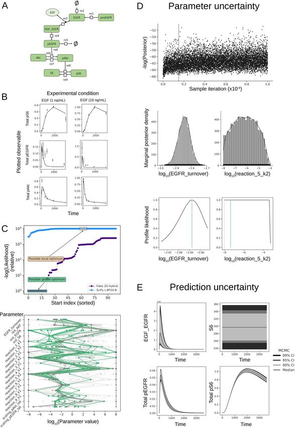
STEP 1.1: Structural identifiability analysis
We first assess structural identifiability and observability for each individual experimental condition,
obtaining a different subset of identifiable parameters for each one. Next, we repeat the analysis
after combining the information from all experiments, obtaining that all parameters are structurally
identifiable. However, the two state variables that are not measured in any experiment (β-io and
OH-β-io) are not observable. If the initial conditions of these two states were considered as unknown
parameters, they would be non-identifiable.
STEP 1.2: Address structural non-identifiabilities
We are not interested in the two unobservable states. Hence we omit this step, and proceed with the
original model.
16Figure 5: Calibration of the carotenoid pathway model. (A) Schematic of the model pathway. (B)
Visualization of the fit. The plot shows the trajectories of the model observables, as well as the means (points)
and standard errors of the means (error bars) of the measurements. (C) Upper: A waterfall plot, showing the
number of starts that converged to the MLE. Here and in the remaining subfigures, green indicates results that
correspond to the MLE. Lower: A parameters plot, showing variability of parameters among starts that converged
to the possible global optimum (green). Vertical dotted lines indicate parameter bounds. (D) Plots related to
parameter uncertainty analysis. Upper: a trace of the function values of samples from a MCMC chain. The
vertical dotted line indicates burn-in. Middle: marginal density distributions of two parameters, using samples
17 estimate, histogram, and rug plot. Lower: profiled
from the converged chain. The plots show a kernel density
likelihood of two parameters. (E) Plots related to prediction uncertainty analysis, computed as percentiles from
predictions of samples. Upper: prediction uncertainties of two states. Lower: prediction uncertainties of two
observables. Note that in this model, observables are states without transformation, hence the observables and
states have the same uncertainties.STEP 2.1: Objective function
We use the negative log-likelihood objective function described in Equation 2, which is the common
choice in frequentist approaches.
STEP 3.1 and 3.2: Parameter optimisation
We estimate model parameters using the multi-start local optimisation method L-BFGS-B imple-
mented in the Python package SciPy. With 100 starting points we achieve convergence to the max-
imum likelihood estimate, as indicated in the waterfall plot (Fig. 5). The parameters plot shows
that the parameter vector is similar amongst the best starts, indicating that the parameters are
well-determined by the optimisation problem and the optimiser.
STEP 4.1: Assess goodness of fit
Visual inspection indicates a good quality of the fit, with simulations closely matching measurements.
STEP 4.2: Address fit issues
As the fit is good, this step is skipped.
STEP 5.1: Practical identifiability analysis
We analyse practical identifiability using profile likelihoods and MCMC sampling. Profile likelihoods
suggest that all parameters are practically identifiable, as the confidence intervals span relatively small
regions of the parameter space. The profiles peak at the maximum likelihood estimate (MLE), sug-
gesting that optimisation was successful. MCMC sampling yields similar results; parameter marginal
distributions span a similar distance of parameter space compared to profile likelihoods, and credi-
bility intervals are also similar.
STEP 6.1: Prediction uncertainty analysis
We calculate credibility intervals using ensembles of parameters from sampling. In this model, there
is a one-to-one correspondence between states and observables, hence the plots are the same. The
prediction uncertainties are reasonably low, suggesting that the model has been successfully calibrated
and might be used to predict new behaviour.
Akt pathway model
The second example is an AKT pathway model [27] with 22 unknown parameters, 3 of which are
unknown initial conditions, 9 state variables, 3 outputs, and 1 input. There are 6 experimental
conditions, each of them with a different input EGF concentration.
Results are summarised in the following paragraphs and in Fig. 6.
STEP 1.1: Structural identifiability analysis
We consider the following scenarios:
1. For a single experiment with constant EGF, 11 parameters are structurally non-identifiable, and
3 states are unobservable.
2. For a single experiment with time-varying EGF, the model becomes structurally identifiable
and observable.
18Figure 6: Calibration of the Akt pathway model. (A) Schematic of the model pathway. (B) Visualization of
the fit. The plot shows the trajectories of the model observables, as well as the means (points) and standard errors
of the means (error bars) of the measurements. (C) Upper: A waterfall plot, showing the number of starts that
converged to the MLE. Here and in the remaining subfigures, green indicates results that correspond to the MLE.
19
Lower: A parameters plot, showing variability of parameters among starts that converged to the possible global
optimum (green). Vertical dotted lines indicate parameter bounds. (D) Plots related to parameter uncertainty
analysis. Upper: a trace of the function values of samples from an MCMC chain. The vertical dotted line indicates
burn-in. Middle: marginal density distributions for two parameters, using samples from the converged chain. The
plots show a kernel density estimate, histogram, and rug plot. Lower: profiled likelihood of two parameters. The
dotted vertical line indicates a parameter bound. (E) Plots related to prediction uncertainty analysis, computed
as percentiles from predictions of samples. Upper: prediction uncertainties of two states under one experimental
condition. Lower: prediction uncertainties of two observables under one experimental condition.3. For multiple experiments (at least two) with constant EGF, the model is structurally identifiable
and observable.
The experimental data available corresponds to the scenario (3) above. The scenario (2) yields an
identifiable and observable model, but it requires a continuously varying value of EGF, which is not
practical. It is also interesting to note the role of initial conditions in this case study. The results
summarised above are obtained with generic (nonzero) initial conditions. However, in the available
experimental datasets there are several initial conditions equal to zero. Introducing this assumption
in the analyses of the scenarios (2) and (3) leads to a loss of identifiability and observability: four
parameters become non-identifiable and one state becomes unobservable.
STEP 1.2: Address structural non-identifiabilities
We assume a realistic scenario corresponding to the available experimental data: several experimental
conditions with a constant input, EGF, and certain initial conditions equal to zero. In this case the
model has four non-identifiable parameters and one unobservable state. To make the model fully
observable and structurally identifiable, it is necessary and sufficient to fix the value of two of the
non-identifiable parameters. Thus, we fix two of these parameters and proceed with the next steps.
For comparison, we also performed the remaining steps without fixing the non-identifiable param-
eters. We found that fixing the non-identifiability issues resulted in slightly faster and more robustly
convergent optimisations, as well as in better practical identifiability and reduced state uncertainty.
STEP 2.1: Objective function
We choose the negative log-likelihood objective function described in Equation 2.
STEP 3.1 and 3.2: Parameter optimisation
Similarly to the other case study, we initially use the multi-start local optimisation method “L-BFGS-
B”.
STEP 4.1: Assess goodness of fit
Visual inspection (i.e. comparison of the simulations produced by the maximum likelihood estimate
with the measurements) reveals a poor fit to the data (not shown). This result is obtained even with
the best result obtained from thousands of optimisation runs from different starting points.
STEP 4.2: Address fit issues
First we try to improve the fit by tuning the settings of the optimisation method, L-BFGS-B, without
success. Then we try a different method, Fides, which has a higher computational cost but achieves
higher quality steps during optimisation. With Fides we find an MLE that produces a fit comparable
to the one reported in the original publication. The high number of starts (in the order of 103 )
required to find this fit reproducibly indicates that this is a difficult parameter optimisation problem.
STEP 5.1: Practical identifiability analysis
Credibility intervals obtained from MCMC sampling indicate that several parameters are practically
non-identifiable. This result is not significantly improved by fixing parameters as suggested in STEP
1.2. Improving the practical identifiability of these parameters would require repeating the calibration
with additional experimental data.
20You can also read