Identification of brain states, transitions, and communities using functional MRI
←
→
Page content transcription
If your browser does not render page correctly, please read the page content below
Identification of brain states, transitions, and communities using
functional MRI
a,b,*
Lingbin Bian , Tiangang Cui a , B.T. Thomas Yeoc , Alex Fornito b , Adeel Razi b,d,+,*
and Jonathan Keith a,+
a
School of Mathematics, Monash University, Australia
b
Turner Institute for Brain and Mental Health, School of Psychological Sciences and Monash Biomedical Imaging, Monash
University, Australia
c
Department of Electrical and Computer Engineering, National University of Singapore, Singapore
d
Wellcome Centre for Human Neuroimaging, University College London, United Kingdom
+
Joint senior authors
arXiv:2101.10617v1 [q-bio.NC] 26 Jan 2021
*
Corresponding authors: Lingbin Bian (lingbin.bian@monash.edu) and Adeel Razi (adeel.razi@monash.edu)
Abstract Markov model to explore dynamic jumps between discrete
brain states and found that the variations in the sensory and
narrative properties of the movie can evoke discrete brain
Brain function relies on a precisely coordinated and dynamic
processes [14]. Task-fMRI studies with more restrictive con-
balance between the functional integration and segregation
straints on stimuli have demonstrated that functional con-
of distinct neural systems. Characterizing the way in which
nectivity exhibits variation during motor learning [15] and
neural systems reconfigure their interactions to give rise to
anxiety-inducing speech preparation [16]. Although task-
distinct but hidden brain states remains an open challenge.
based fMRI experiments can, to some extent, delineate the
In this paper, we propose a Bayesian model-based character-
external stimuli (for example, the onset and duration of
ization of latent brain states and showcase a novel method
stimuli in the block designed experiments), which constitute
based on posterior predictive discrepancy using the latent
reference points against which to identify changes in the ob-
block model to detect transitions between latent brain states
served signal, this information does not precisely determine
in blood oxygen level-dependent (BOLD) time series. The
the timing and duration of the latent brain state relative
set of estimated parameters in the model includes a latent
to psychological processes or neural activity. For example,
label vector that assigns network nodes to communities, and
an emotional stimulus may trigger a neural response which
also block model parameters that reflect the weighted con-
is delayed relative to stimulus onset and which persists for
nectivity within and between communities. Besides exten-
some time after stimulus offset. Moreover, the dynamics of
sive in-silico model evaluation, we also provide empirical
brain states and functional networks are not induced only
validation (and replication) using the Human Connectome
by external stimuli, but also by unknown intrinsic latent
Project (HCP) dataset of 100 healthy adults. Our results ob-
mental processes [17]. Therefore, the development of non-
tained through an analysis of task-fMRI data during working
invasive methods for identifying transitions of latent brain
memory performance show appropriate lags between exter-
states during both task performance and task-free conditions
nal task demands and change-points between brain states,
is necessary for characterizing the spatiotemporal dynamics
with distinctive community patterns distinguishing fixation,
of brain networks.
low-demand and high-demand task conditions.
Change-point detection in multivariate time series is a sta-
tistical problem that has clear relevance to identifying tran-
sitions in brain states, particularly in the absence of knowl-
edge regarding the experimental design. Several change-
identifying changes in brain connectivity over time point detection methods based on spectral clustering [18, 19]
I can provide insight into fundamental properties of hu-
man brain dynamics. However, the definition of dis-
crete brain states and the method of identifying the states
and dynamic connectivity regression (DCR) [16] have been
previously developed and applied to the study of fMRI time
series, and these have enhanced our understanding of brain
has not been commonly agreed [1]. Experiments targeting dynamics. However, change-point detection with spectral
unconstrained spontaneous ‘resting-state’ neural dynamics clustering only evaluates changes to the component eigen-
[2, 3, 4, 5, 6, 7, 8, 9, 10] have limited ability to infer latent structures of the networks but neglects the weighted connec-
brain states or determine how the brain segues from one tivity between nodes, while the DCR method only focuses
state to another because it is not clear whether changes in on the sparse graph but ignores the modules of the brain
brain connectivity are induced by variations in neural ac- networks Other change-point detection strategies include a
tivity (for example induced by cognitive or vigilance states) frequency-specific method [20], applying a multivariate cu-
or fluctuations in non-neuronal noise [11, 12, 13]. A re- mulative sum procedure to detect change-points using EEG
cent study with naturalistic movie stimuli used a hidden data, and methods which focus on large scale network es-
1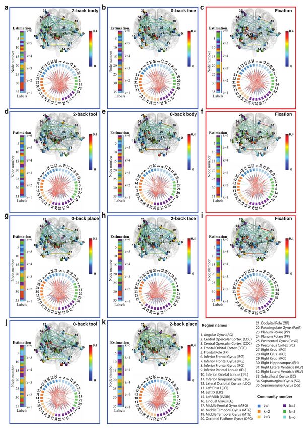
timation in fMRI time series [21, 22, 23, 24]. Many fMRI             contrast to the stochastic block model used in time-varying
studies use sliding window methods for characterizing the            functional connectivity studies, the Gaussian latent block
time-varying functional connectivity in time series analysis         model used in our work considers the correlation matrix as
[2, 8, 25, 26, 27, 28, 29]. Methods based on hidden Markov           an observation without imposing any arbitrary thresholds,
models (HMM) are also widely used to analyze transient               so that all the information contained in the time series is
brain states [30, 31, 32].                                           preserved, resulting in more accurate detection of change-
   A community is defined as a collection of nodes that are          points. Moreover, unlike methods based on fixed commu-
densely connected in a network. The problem of commu-                nity memberships over the time course [38], our methods
nity detection is a topical area of network science [33, 34].        consider both the community memberships and parameters
How communities change or how the nodes in a network                 related to the weighted connectivity to be time varying,
are assigned to specific communities is an important prob-           which results in more flexible estimation of both commu-
lem in the characterization of networks. Although many               nity structure and connectivity patterns. Furthermore, our
community detection problems in network neuroscience are             Bayesian change-point detection method uses overlapping
based on modularity [15, 35, 36], recently a hidden Markov           sliding windows that assess all of the potential candidate
stochastic block model combined with a non-overlapping               change-points over the time course, which increases the res-
sliding window was applied to infer dynamic functional con-          olution of the detected change-points compared to methods
nectivity for networks, where edge weights were only binary          using non-overlapping windows [37, 38]. Finally, the pro-
and the candidate time points evaluated were not consecu-            posed Bayesian change-point detection method is computa-
tive [37, 38]. More general weighted stochastic block mod-           tionally efficient, scaling to whole-brain networks potentially
els [39] have been used to infer structural connectivity for         covering hundreds of nodes within a reasonable time frame
human lifespan analysis [40] and to infer functional connec-         in the order of tens of minutes.
tivity in the mesoscale architecture of drosophila, mouse,              Our paper presents four main contributions, namely: (i)
rat, macaque, and human connectomes [41]. However, these             we quantitatively characterize discrete brain states with
studies using the weighted stochastic block model only ex-           weighted connectivity and time-dependent community mem-
plore the brain network over the whole time course of the            berships, using the latent block model within a tempo-
experiment and neglect dynamic properties of networks.               ral interval between two consecutive change-points; (ii) we
Weighted stochastic block models [39] are described in terms         propose a new Bayesian change-point detection method
of exponential families (parameterized probability distribu-         called posterior predictive discrepancy (PPD) to estimate
tions), with the estimation of parameters performed using            transition locations between brain states, using a Bayesian
variational inference [42, 43]. Another relevant statistical         model fitness assessment; (iii) in addition to the locations
approach introduces a fully Bayesian latent block model              of change-points, we also infer the community architecture
[2, 3], which includes both a binary latent block model and a        of discrete brain states, which we show are distinctive of 2-
Gaussian latent block model as special cases. The Gaussian           back, 0-back, and fixation conditions in a working-memory
latent block model is similar to the weighted stochastic block       task-based fMRI experiment, and; (iv) we further empir-
model, but different methods have been used for parameter            ically find that the estimated change-points between brain
estimation, including Markov chain Monte Carlo (MCMC)                states show appropriate lags compared to the external work-
sampling.                                                            ing memory task conditions.
   Although there is a broad literature exploring change-
point detection, and also many papers that discuss com-
munity detection, relatively few papers combine these ap-            Results
proaches, particularly from a Bayesian perspective. In this
paper, we develop Bayesian model-based methods which                 Our proposed method is capable of identifying transitions
unify change-point detection and community detection to              between discrete brain states and infer the patterns of con-
explore when and how the community structure of discrete             nectivity between brain regions that underlie those brain
brain state changes under different external task demands at         states by modelling time-varying dynamics in BOLD sig-
different time points using functional MRI. There are several        nal under different stimuli. In this section, we validate our
advantages of our approach compared to existing change-              proposed methodology by applying Bayesian change-point
point detection methods. Compared to data-driven methods             detection and network estimation to both synthetic data
like spectral clustering [18, 19] and DCR [16], which either         and real fMRI data. The Bayesian change-point detection
ignore characterizing the weighted connectivity or the com-          method is described in Fig. 1 and the mathematical formu-
munity patterns, the fully Bayesian framework and Markov             lation and detailed descriptions are in the Methods section
chain Monte Carlo method provide flexible and powerful               (also see Supplementary information). We first use syn-
strategies that have been under-used for characterizing the          thetic multivariate Gaussian data for extensive validation
latent properties of brain networks, including the dynamics          and critically evaluate the performance of our change-point
of both the community memberships and weighted connec-               detection and sampling algorithms. For real data analysis,
tivity properties of the nodal community structures. Exist-          we use working memory task fMRI (WM-tfMRI) data from
ing change-point detection methods based on the stochastic           the Human Connectome Project (HCP) [46]. We extracted
block model all use non-overlapping sliding windows and              the time series of 35 nodes whose MNI coordinates were de-
were applied only to binary brain networks [37, 38]. In              termined by significant activations obtained via clusterwise

                                                                 2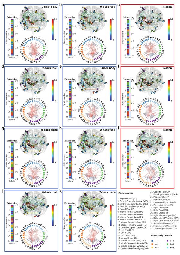
Fig. 1: The framework for identifying brain states, transitions and communities: a Schematic of the proposed Bayesian change-point detection
method. Three different background colors represent three brain states of individual subjects with different community architectures. The
colors of the nodes represent community memberships. A sliding window of width W centered at t is applied to the time series. The different
colored time series correspond to BOLD time series for each node. The sample correlation matrix xt (i.e., an observation for our Bayesian
model) is calculated from the sample data Yt within the sliding window. We use the Gaussian latent block model to fit the observations
and evaluate model fits to the observations to obtain the posterior predictive discrepancy index (PPDI). We then calculate the cumulative
discrepancy energy (CDE) from the PPDI and use the CDE as a scoring criterion to estimate the change-points of the community architectures.
b Dynamic community memberships of networks with N = 16 nodes. A latent label vector z contains the labels (k) of specific communities
for the nodes. Nodes of the same color are located in the same community. The dashed lines represent the (weighted) connectivity between
communities and the solid lines represent the (weighted) connectivity within the communities. c Model fitness assessment. The observation
is the realized adjacency matrix; different colors in the latent block model represent different blocks with the diagonal blocks representing
the connectivity within a community and the off-diagonal blocks representing the connectivity between communities. To demonstrate distinct
blocks of the latent block model, in this schematic we group the nodes in the same community adjacently and the communities are sorted. In
reality, the labels of the nodes are mixed with respect to an adjacency matrix. The term πkl represents the model parameters in block kl.

                                                                     3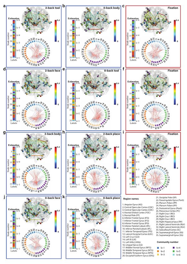
Fig. 2: Results of method validation using synthetic data: a CDE of the multivariate Gaussian data with SNR=5dB using different models
(K=6, 5, 4, and 3). The sliding window size for converting from time series to correlation matrices sequence is W = 20, whereas (for smoothing)
the sliding window size for converting from PPDI to CDE is Ws = 10. The vertical dashed lines are the locations of the true change-points
(t=20, 50, 80, 100, 130, and 160). The colored scatterplots in the figures are the CDEs of individual (virtual) subjects and the black curve is
the group CDE (averaged CDE over 100 subjects). The red points are the local maxima and the blue points are the local minima. b Local
fitting with different models (from K=3 to 18) for synthetic data (SNR=5dB). Different colors represent the PPDI values of different states
with the true number of communities K true . c The estimation of community constituents for SNR=5dB at each discrete state: t=36, 66, 91,
116, 146) for brain states 1 to 5, respectively. The estimations of the latent label vectors (Estimation) and the label vectors (True) that
determine the covariance matrix in the generative model are shown as bar graphs. The strength and variation of the connectivity within and
between communities are represented by the block mean and variance matrices within each panel.

                                                                      4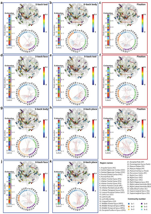
inference using FSL [47].                                            models are also included in this figure. We use the most
                                                                     frequent latent label vectors in the Markov chain after the
                                                                     burn-in steps as the estimate. Note that label-switching oc-
Method validation using synthetic data                               curs in the MCMC sampling, which is a well-known prob-
To validate the Bayesian change-point detection algorithm,           lem in Bayesian estimation of mixture models [1]. In the
we first use synthetic data with the signal to noise ratio           results presented here, the node memberships have been re-
(SNR)=5dB. The simulated states of segments between two              labelled to correct for label switching. The algorithm used
true change-points in the synthetic data could be repeat-            for this purpose is described in Supplementary Section 2.
ing or all different, depending on the settings of the pa-           We find that the estimated latent label vectors are (largely)
rameters in the generative model. A detailed description             consistent with the ground truth of labels that determined
of the generative model and parameter settings for simu-             the covariance matrix. The discrepant ‘True’ and ‘Estima-
lating the synthetic data are provided in Supplementary              tion’ patterns with respect to states 2 and 4 are due to the
Section 1. Further simulation results with different lev-            bias induced by the selected model (K = 5 for the ground
els of SNR (SNR=10dB, SNR=0dB, and SNR=-5dB) are                     truth and K = 4 for the selected model). Although the
provided in Supplementary Figures 1, 2, and 3. The                   colors of the labels in the ‘True’ and ‘Estimation’ patterns
resulting group-level cumulative discrepancy energy (CDE)            are discrepant, we can see that the values of the labels are
scores (see Methods section for how we define CDE) using             largely consistent, with some labels of k = 5 missing in the
models with different values of K, where K is the number             ‘Estimation’ pattern compared to the ‘True’ pattern.
of communities, are shown in Fig. 2a. We use a latent                   Given the estimated latent label vector, we then draw
block model to fit the adjacency matrix at consecutive time          samples of the block mean and variance from the posterior
points for change-point detection, which we call global fit-         p(π|x, z) conditional on the estimated latent label vector
ting. The local maxima (red dots) of the group CDE indi-             z. However, there is no ground truth for the block mean
cate locations of change-points and the local minima (blue           and variance when we generate the synthetic data. The
dots) correspond to distinct states that differ in their com-        validation of sampling model parameters is illustrated in the
munity architecture. We find that the local maxima (red              Supplementary Figure 4.
dots) are located very close to the true change-points in all
of the graphs (in Fig. 2a) which means that the global fitting       Method validation using working memory
has good performance. Here we clarify that global fitting is
used to estimate the locations of the change-points or tran-
                                                                     (WM) task-fMRI data
sitions of brain states, and local fitting is used to select a       In this analysis, we used preprocessed working memory
latent block model to estimate the community structures of           (WM)-tfMRI data obtained from 100 unrelated healthy
discrete brain states (see Methods section for a detailed            adult subjects under a block designed paradigm, available
explanation of global and local fitting).                            from the Human Connectome Project (HCP) [46]. We
   Next, using the global fitting results, with K = 6 and            mainly focused on the working memory load contrasts of
W = 20, where W is the width of the sliding (rectangular)            2-back vs fixation, 0-back vs fixation, or 2-back vs 0-back,
window, we find the local minima (the blue dots) locations           and determine the brain regions of interest from the GLM
to be t = {36, 66, 91, 116, 146}, where each location corre-         analysis. After group-level GLM analysis, we obtained clus-
sponds to a discrete state. Next, we use local fitting to            ter activations with locally maximum Z statistics for differ-
select a model (i.e. K for local inference) to infer the com-        ent contrasts. The results in the form of thresholded local
munity membership and model parameters relating to the               maximum Z statistic (Z-MAX) maps are shown in Supple-
connectivity of the discrete states. For local inference, the        mentary Figure 5. The light box views of thresholded
group averaged adjacency matrix is considered as the obser-          local maximum Z statistic with different contrasts are pro-
vation. We assess the goodness of fit between observation            vided in Supplementary Figures 6. Significant activa-
and a latent block model with various values of K (from              tions obtained by clusterwise inference and the correspond-
K = 3, · · · , 18) using posterior predictive discrepancy for        ing MNI coordinates with region names are shown in Table
each local minimum, as shown in Fig. 2b. We selected the             1. We finally extracted the time series of 35 brain regions
value of K at which the curve starts to flatten as the pre-          corresponding to the MNI coordinates. Refer to Methods
ferred model. We find that the model assessment curves for           section for the details of experimental design, GLM analysis
states 1, 2, 4, and 5 flatten at K = 4, whereas the model            and time series extraction.
assessment curve for state 3 is flat over the entire range
(from K = 3 and up). Therefore the selected models are
                                                                     Change-point detection for tfMRI time series
K = {4, 4, 3, 4, 4} for states 1 to 5, respectively.
   To validate the MCMC sampling of the density p(z|x, K),           In the main text, we illustrate the results using the HCP
we compare the estimate of the latent label vector to the            working memory data of session 1 i.e. with the polarity of
ground truth of the node memberships. Fig. 2c shows the              Left to Right (LR). The replication of results obtained by
inferred community architectures of the discrete states in-          using session 2 (RL) are demonstrated in Supplementary
cluding the estimated latent label vectors and the model             Figures 10 to 15) and Supplementary Table 1. We
parameters of block mean and variance. The true label vec-           compare the brain states of different working memory loads
tors that determine the covariance matrix in the generative          for a specific kind of picture (tool, body, face, and place)

                                                                 5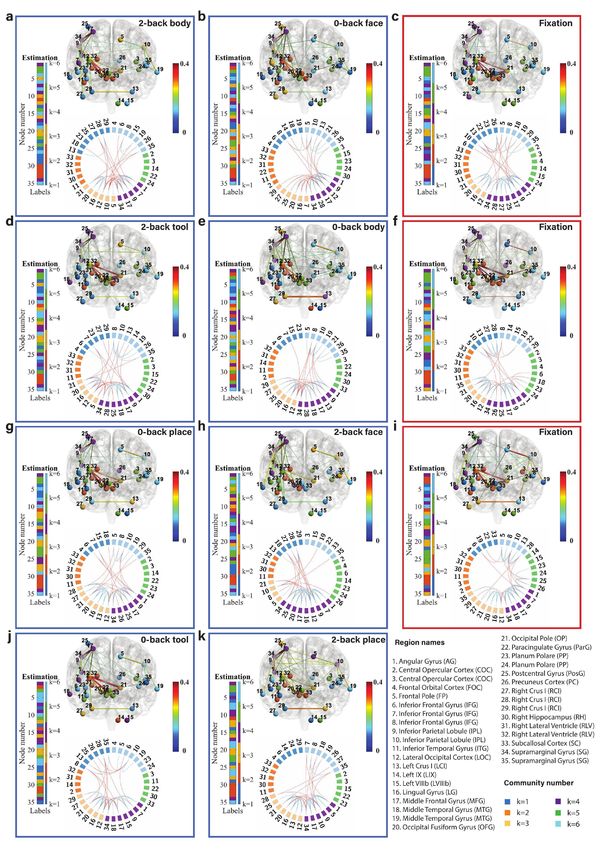
MNI   coordinates     Voxel locations
              Node number       Z-MAX       x     y     z         x   y     z          Region name
              1                 4.97        48    -58 22          21 34 47             Angular Gyrus
              2                 9.61        36    8     12        27 67 42             Central Opercular Cortex
              3                 8.27        -36   4     12        63 65 42             Central Opercular Cortex
              4                 6.48        40    34    -14       25 80 29             Frontal Orbital Cortex
              5                 7.83        -12   46    46        51 86 59             Frontal Pole
              6                 4.84        54    32    -4        18 79 34             Inferior Frontal Gyrus
              7                 6           52    38    10        19 82 41             Inferior Frontal Gyrus
              8                 4.38        -52   40    6         71 83 39             Inferior Frontal Gyrus
              9                 6.05        52    -70 36          19 28 54             Inferior Parietal Lobule PGp R
              10                7.26        -48   -68 34          69 29 53             Inferior Parietal Lobule PGp L
              11                6.18        44    -24 -20         23 51 26             Inferior Temporal Gyrus
              12                9.54        36    -86 16          27 20 44             Lateral Occipital Cortex
              13                8.04        -30   -80 -34         60 23 19             Left Crus I
              14                7.6         -8    -58 -52         49 34 10             Left IX
              15                6.9         -22   -48 -52         56 39 10             Left VIIIb
              16                14.5        6     -90 -10         42 18 31             Lingual Gyrus
              17                10.3        30    10    58        30 68 65             Middle Frontal Gyrus
              18                6.61        66    -30 -12         12 48 30             Middle Temporal Gyrus
              19                4.53        -68   -34 -4          79 46 34             Middle Temporal Gyrus
              20                14.5        18    -88 -8          36 19 32             Occipital Fusiform Gyrus
              21                5.06        -12   -92 -2          51 17 35             Occipital Pole
              22                9.87        6     40    -6        42 83 33             Paracingulate Gyrus
              23                12          42    -16 -2          24 55 35             Planum Polare
              24                11.3        -40   -22 0           65 52 36             Planum Polare
              25                9.03        38    -26 66          26 50 69             Postcentral Gyrus
              26                8.31        -10   -60 14          50 33 43             Precuneus Cortex
              27                5.7         46    -60 -42         22 33 15             Right Crus I
              28                8.34        32    -80 -34         29 23 19             Right Crus I
              29                10.9        32    -58 -34         29 34 19             Right Crus I
              30                6.41        10    -8    -14       40 59 29             Right Hippocampus
              31                6.19        32    -52 2           29 37 37             Right Lateral Ventricle
              32                7.69        24    -46 16          33 40 44             Right Lateral Ventricle
              33                6.13        0     10    -14       45 68 29             Subcallosal Cortex
              34                10.7        48    -44 46          21 41 59             Supramarginal Gyrus
              35                4.23        -50   -46 10          70 40 41             Supramarginal Gyrus

Table 1: Significant activations of cluster wise inference (cluster-corrected Z>3.1, P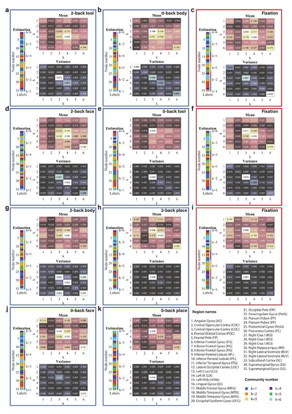
Fig. 3: The results of Bayesian change-point detection for working memory tfMRI data (session 1, LR): Cumulative discrepancy energy
(CDE) with different sliding window sizes (W =22, 26, 30, and 34; a-d under the model K = 3) and different models (K=3, 4, and 5; c, e and
f using a sliding window of W = 30). Ws is width of the sliding window used for converting from PPDI to CDE. The vertical dashed lines
are the times of onset of the stimuli, which are provided in the EV.txt files in the released data. The multi-color scatterplots in the figures
represent the CDEs of individual subjects and the black curve is the group CDE (averaged CDE over 100 subjects). The red dots are the local
maxima, which are taken to be the locations of change-points, and the blue dots are the local minima, which are used for local inference of the
discrete brain states.

Larger values of K imply more blocks in the model, which                  transforming from PPDI to CDE. A larger window size (for
gives rise to relatively better model fitness. In this situation,         example Ws = 30) reduces the accuracy of the estimates
there will be less distinction between relatively static brain            and results in false negatives. Too small a value of Ws in-
states and transition states with change-points in the win-               creases the false positive rate. We found that Ws = 10 works
dow. The false positives among the local minima and local                 well for all of the real data analyses. The time spent to run
maxima are also influenced by the window size Ws used for                 the posterior predictive assessment on each subject (T =405

                                                                      7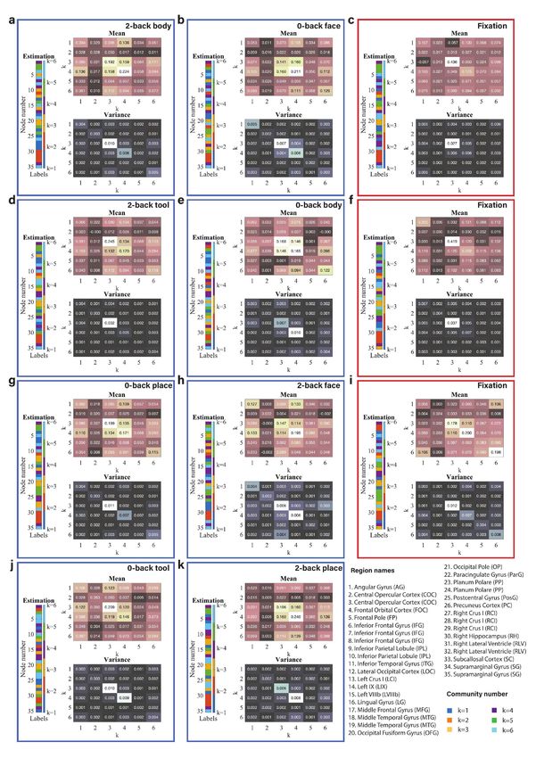
Fig. 4: Detected change-points and the locations of brain states matching the task blocks for working memory tfMRI data (session 1, LR)
with K = 3, and W = 30. The numbers in the small rectangular frame are the boundaries of the external task demands, the background
colors in the large rectangular are the different task conditions, and the blue and red bars with specified numbers are the estimated locations
of discrete brain states and change-points.

frames, posterior predictive replication number S=50, K=3, mated time points of the discrete brain states (minima) are
and the window size W =30) by using a 2.6 GHz Intel Core {41, 76, 140, 175, 239, 278, 334, 375}. A comparison of the de-
i7 processor unit was about 10 minutes.                    tected change-points to the task blocks for working memory
                                                           tfMRI data are shown in Fig. 4.

                                                                              Local inference for discrete brain states
                                                                              For ‘local inference’, we first calculated the group averaged
                                                                              adjacency matrix with a window of Wg = 20, for all brain
                                                                              states. The center of the window is located at the time point
                                                                              of the local minimum value. We evaluated the goodness of
                                                                              fit for models with different values of K (Fig. 5). The re-
                                                                              sults demonstrate that the goodness of fit trends to flat at
                                                                              K = 6. To avoid empty communities, K = 6 is then selected
                                                                              as the number of communities in local inference. Note that
                                                                              the value of K is unchanged in Markov chain Monte Carlo
                                                                              estimation, but an empty community containing no labels
                                                                              may take place. In the remainder of this section, we used
                                                                              the model with K = 6 for all brain states. The times spent
                                                                              to run the estimation for latent label vector and model pa-
Fig. 5: Local fitting between averaged adjacency matrix and models            rameters for a single discrete brain state (MCMC sampling
from K=3 to 18. Different colors represent the PPDI values of different       number Ss =200, K=6, and the window size W =20) by us-
brain states.                                                                 ing a 2.6 GHz Intel Core i7 processor unit were about 1.85
                                                                              and 1.25 seconds respectively.
   The ‘local inference’ is defined as a way to estimate the                     The inferred community structures are visualized using
discrete brain state corresponding to each task condition                     BrainNet Viewer [49] and Circos maps [50] as shown in Fig.
via Bayesian modelling. The group averaged dynamic func-                      6. Estimated latent label vectors are visualized using dif-
tional networks were analyzed by performing ‘local infer-                     ferent colors to represent different communities. The nodes
ence’ as follows. In this experiment, we used results ob-                     are connected by weighted links at a sparsity level of 10%
tained for K = 3 and W = 30 (see Fig. 3c). We first                           (we also visualized the brain states with sparsity levels of
listed all of the local maxima and minima, where the time                     20% and 30%: Supplementary Figures 7 and 8). The
points with distances smaller than 8 are grouped as vec-                      density and variation of connectivity within and between
tors. Maxima and minima deemed to be false positives                          communities are characterized by the estimated block mean
were discarded. The time points corresponding to the lo-                      matrix and block variance matrix in Supplementary Fig-
cal minimum value of group CDE are (41, 46, 48, 50,                           ure 9 and 15. We first describe the working memory tasks
54) and (140, 147, 152). These were determined as single                      involving the 2-back tool (Fig. 6a), 0-back tool (Fig. 6e),
time points corresponding to discrete brain states, specif-                   and fixation (Fig. 6c, f, i). The locations of fixation states
ically 41 and 140 respectively, with all the other elements                   are considered as the locations of the change-points at 107,
in the vectors presumed to be false positives and discarded.                  206, and 306 (we consider the fixation state as a transition
Time points with CDE value difference smaller than 0.002                      buffer between two working memory blocks). We found that
were also discarded (points (191, 192) and (290, 292)).                       the connectivity between the inferior parietal lobule (node
Then the resulting estimated change-point locations (max-                     9) and middle frontal gyrus (node 17), and the connectiv-
ima) are at {68, 107, 165, 206, 265, 306, 356}, and the esti-                 ity between the inferior parietal lobule (node 9) and supra-

                                                                          8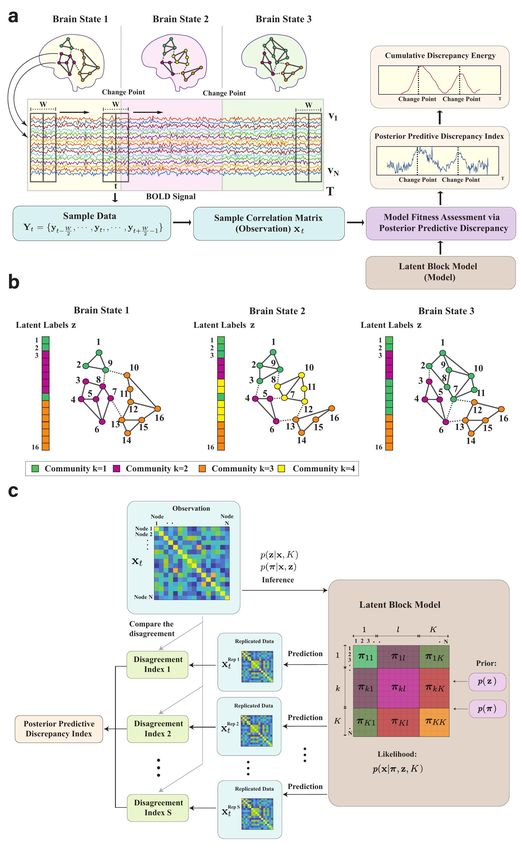
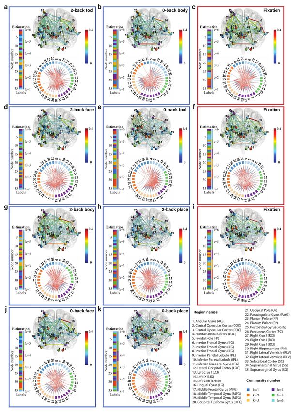
Fig. 6: Community structure of the discrete brain states: The figures with blue frames represent brain states corresponding to working
memory tasks (2-back tool at t = 41; 0-back body at t = 76; 2-back face at t = 140; 0-back tool at t = 175; 2-back body at t = 239; 2-back place
at t = 278; 0-back face at t = 334; and 0-back place at t = 375 in a-k) and those with red frames represent brain states corresponding to fixation
(fixation at t=107, 206, and 306 in c, f, and i). Each brain state shows connectivity at a sparsity level of 10%. The different colors of the labels
represent community memberships. The strength of the connectivity is represented by the colors shown in the bar at the right of each frame.
In Circos maps, nodes in the same community are adjacent and have the same color. Node numbers and abbreviations of the corresponding
brain regions are shown around the circles. In each frame, different colors represent different community numbers. The connectivity above the
sparsity level is represented by arcs. The blue links represent connectivity within communities and the red links represent connectivity between
communities.

                                                                         9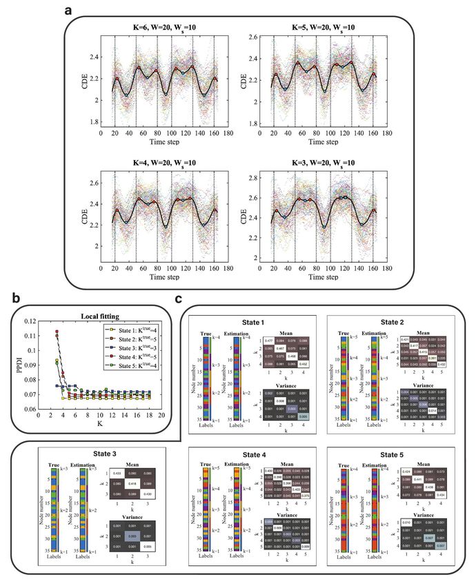
marginal gyrus (node 34) are increased significantly both in         We first focus on the results of the brain states inferred
2-back and 0-back working memory compared to fixation.            from the WM-tfMRI data and discuss the estimated pat-
   For 2-back face (Fig. 6d) and 0-back face (Fig. 6j), The       terns of connectivity for different blocks of working memory
connectivity between inferior parietal lobule (node 9) and        tasks after local inference. We find that there are distinct
supramarginal gyrus (node 34) and the connectivity between        connectivity differences between 2-back, 0-back, and fixa-
angular gyrus (node 1) and supramarginal gyrus (node 34)          tion. We first compare the working memory and the fixation
are increased in 2-back compared to 0-back and fixation.          conditions, with particular reference to the middle frontal
There is reduced connectivity between the lateral occipital       gyrus (node 17) and inferior parietal lobule (node 9) which
cortex (node 12), occipital fusiform gyrus (node 20), and         includes the angular gyrus (node 1) and supramarginal gyrus
occipital pole (node 21) in 2-back and 0-back compared to         (node 34). The middle frontal gyrus is related to manipu-
fixation. There is reduced connectivity between the frontal       lation, distractor resistance, refreshing, selection for action
pole (node 5) and inferior parietal lobule (node 10) only in      and monitoring, and the inferior parietal lobule is related
2-back.                                                           to focus recognition and long-term recollection [51]. In our
   For task blocks with body parts pictures (Fig. 6g and          results, we find that the connectivity between the middle
Fig. 6b), we found that the connectivity between inferior         frontal gyrus and inferior parietal lobule is increased in the
parietal lobule (node 9) and middle frontal gyrus (node 17),      working memory tasks compared to the fixation state. The
and the connectivity between inferior parietal lobule (node       connectivity between the lateral occipital cortex (node 12)
9) and supramarginal gyrus (node 34) are increased signif-        and occipital fusiform cortex (node 21) is strong and stable
icantly both in 2-back and 0-back working memory com-             in fixation compared to the working memory tasks, and a
pared to fixation. The connectivity between angular gyrus         higher working memory load may increase the instability of
(node 1) and supramarginal gyrus (node 34) is increased in        this connectivity.
2-back compared to 0-back and fixation. There is reduced             Regarding the difference between 2-back and 0-back work-
connectivity between the lateral occipital cortex (node 12),      ing memory tasks, we focus on the angular gyrus and supra-
occipital fusiform gyrus (node 20), and occipital pole (node      marginal gyrus. In our experimental results, we find that
21) in 2-back and 0-back compared to fixation.                    there is increased connectivity between the angular gyrus
   Finally, we compare 2-back place (Fig. 6h), 0-back place       (node 1) and supramarginal gyrus (node 34) in 2-back com-
(Fig. 6k), and fixation. We found that the connectivity           pared to 0-back working memory task blocks. The angular
between lateral occipital cortex (node 12) and occipital pole     gyrus is located in the posterior part of the inferior parietal
(node 21), and the connectivity between occipital fusiform        lobule. The inferior parietal cortex, including the supra-
gyrus (node 20) and occipital pole (node 21) are reduced in       marginal gyrus and the angular gyrus, is part of a “bottom-
2-back compared to 0-back and fixation.                           up” attentional subsystem that mediates the automatic al-
   It is clear from Fig. 6 that nodes are clustered into com-     location of attention to task-relevant information [52]. Pre-
munities with different connectivity densities within and be-     vious work has shown that activation of the inferior parietal
tween communities. The mean and variance of the connec-           lobe is involved in the shifting of attention towards particu-
tivity within and between communities are reported as block       lar stimuli [53]. The right inferior parietal lobule including
mean and variance matrices in Fig. 6. We find that there          angular gyrus is related to attention maintaining and salient
are strong connections in communities k=3, 4, and 6 and           event encoding in the environment [54]. These research find-
weak connections in communities k=1, 2, and 5 for a ma-           ings are consistent with and justify our results.
jority of the states. The Circos map provides a different            Next, we focus on the methodology. We introduced pos-
perspective on the community pattern of the brain state.          terior predictive discrepancy (PPD), a novel method based
We summarise the common community pattern for specific            on model fitness assessment combined with sliding window
working memory load or fixation in Table 1.                       analysis to detect change-points in various functional brain
                                                                  networks and to infer the dynamics when a brain changes
                                                                  state. Posterior predictive assessment is a method based on
Discussion                                                        Bayesian model comparison. Other Bayesian model compar-
                                                                  ison methods including Bayes factors [55, 56], the Bayesian
We proposed a model-based method for identifying transi-          information criterion (BIC) [57], and Kullback–Leibler di-
tions and characterising brain states between two consecu-        vergence [58] are also widely used in mixture modelling. One
tive transitions. The transitions between brain states identi-    advantage of the posterior predictive assessment is that the
fied by the Bayesian change-point detection method exhibit        computation for the assessment is a straightforward byprod-
appropriate lags compared to the external task demands.           uct of the posterior sampling required in the conventional
This indicates a significant difference between the temporal      Bayesian estimation.
boundaries of external task demands and the transitions of           We defined a new criterion named cumulative discrepancy
latent brain states. We also estimated the community mem-         energy (CDE) to estimate locations of these change-points
bership of brain regions that interact with each other to give    or transitions. The main idea underlying this novel strategy
rise to the brain states. Furthermore, we showed that the es-     is to recognize that the goodness-of-fit between the model
timated patterns of community architectures show distinct         and observation is reduced if there is a change-point located
networks for 2-back and 0-back working memory load and            within the current sliding window (the sample data in the
fixation.                                                         window can be considered as being generated from two la-

                                                             10
2-back 0-back Fixation
Community Node number Community Node number Community Node number
k=1 k=1 k=1
k=2 15 30 k=2 k=2 15 31 32
k=3 16 20 k=3 16 20 21 k=3 12 16 20 21
k=4 1 9 17 34 k=4 k=4 1 9 25
k=5 11 14 k=5 k=5 3 11 14
k=6 8 19 35 k=6 19 k=6 5 8 10 19
Table 2: This table summarises the nodes commonly located in a specific community k for all of the picture types in the working memory
tasks.
tent brain network architectures in this case), resulting in fitting, and was fitted to the group-averaged adjacency ma-
a significant increase in CDE. We use overlapping, rectan- trix in the local fitting. Different choices of π can generate
gular, sliding windows so that all of the time points are different connection patterns in the adjacency matrix. The
included. likelihood is Gaussian and the connectivity is weighted, both
The dynamics of the brain states are not only induced by of which facilitate treating the correlation matrix as an ob-
external stimuli, but also the latent mental process, such as servation, without losing much relevant information from
motivation, alertness, fatigue, and momentary lapse [17]. the time series.
Crucially, directly using the temporal boundaries (onsets We treat both the latent label vector and block model
and durations) associated with predefined task conditions parameters as quantities to be estimated. Changes in com-
to infer the functional networks may not be sufficiently rig- munity memberships of the nodes are reflected in changes
orous and accurate. The boundaries of the task demand are in the latent labels, and changes in the densities and vari-
not the timing and duration of the latent brain state. The ations in functional connectivity are reflected in changes in
estimated change-points in our experiments are consistent the model parameters.
with the working memory task demands but show a delay Empirical fMRI datasets have no ground truth regarding
relative to the onsets of the task blocks or the mid-points of the locations of latent transitions of the brain states and
fixation blocks. These results reflect the delay involved due network architectures. Although the task data experiments
to the haemodynamic response, and also the delay arising include the timings of stimuli, the exact change-points be-
from recording the data using the fMRI scanner, between tween discrete latent brain states are uncertain. Here, we
signal emission and reception. used the multivariate Gaussian model to generate synthetic
The results of the task fMRI data analysis show that the data (ground truth) to validate our proposed algorithms
change-point detection algorithm is sensitive to the choice by comparing ground truth to the estimated change-points
of model. We found that a less complex model (with smaller and latent labels. With extensive experiments using syn-
K) for global fitting gave fewer false positives, so it had bet- thetic data, we demonstrated the very high accuracy of our
ter change-point detection performance than models with method. The multivariate Gaussian generative model can
larger K. Selecting a suitable window size W is also very characterize the community patterns via determining the
important for our method. Too small a window size re- memberships of the elements in the covariance matrix, but
sults in too little information being extracted from the data it is still an unrealistic benchmark. In the future, we will in-
within the window, causing the calculated CDE to fluctu- tegrate the clustering method into the dynamic causal mod-
ate more, making it difficult to discriminate local maxima elling [59, 60] to simulate more biologically realistic synthetic
and local minima in the CDE score time series. Too large a data to validate the algorithm.
window size (larger than the task block length) reduces the There are still some limitations of the MCMC allocation
resolution at which the change-points can be distinguished. sampler [2, 3] which we use to infer the latent label vec-
In the working memory task fMRI data set, the length of tors. When Markov chains are generated by the MCMC
the task block is around 34 frames and the fixation is about algorithm, the latent label vectors typically get stuck in lo-
20 frames. Therefore, we made the window size at most 34 cal modes. This is in part because the Gibbs moves in the
frames to ensure all potential change-points can be distin- allocation sampler only update one element of the latent
guished, and at least 20 frames to ensure the effectiveness of label vector at a time. Although the M3 move (see Supple-
the posterior predictive assessment. In our experiments, we mentary Section 7 for details on the M3 move) updates
used window sizes of 22, 26, 30, and 34, which were all larger multiple elements of the latent label vector, the update is
than the length of the fixation block. This means it was not conditional on the probability ratio of a single reassignment,
possible to detect the two change-points at both ends of fix- which results in similar problems to the Gibbs move. Im-
ation blocks, so we consider the whole fixation block as a proving the MCMC allocation sampler so that it can jump
single change-point (i.e., a buffer between two task blocks). between different local modes, without changing the value of
The latent block model provides a flexible approach to K, is a topic worth exploring. Currently, we use an MCMC
modeling and estimating the dynamical assignment of nodes sampler with a Gibbs move and an M3 move for local in-
to a community. Note that the latent block model was fitted ference as well, keeping K constant. In future work, we
to the adjacency matrix of each individual subject in global will extend the sampler using an absorption/ejection move,
11which is capable of sampling K along with latent labels di- FOV = 208 × 180 mm, 72 slices with isotropic voxels of 2 mm with
rectly from the posterior distribution. a multi-band acceleration factor of 8. Two runs of the tfMRI were
acquired (one right to left, the other left to right).
The label switching phenomenon (see Supplementary
Section 2) does not happen frequently if the chain is stuck
in a local mode. However, the estimated labels in the latent tfMRI data preprocessing
label vector do switch in some experiments. To correct for The tfMRI data in HCP are minimally preprocessed including gradi-
label switching, we permute the labels in a post-processing ent unwarping, motion correction, fieldmap-based EPI distortion cor-
rection, brain-boundary-based registration of EPI to structural T1-
stage. weighted scan, non-linear (FNIRT) registration into MNI152 space,
In this paper, we treat the group-averaged adjacency ma- and grand-mean intensity normalization. The data analysis pipeline
trix as an observation in local inference, which neglects vari- is based on FSL (FMRIB’s Software Library) [47]. Further smoothing
processing is conducted by Volume-based analysis and Grayordinates-
ation between subjects [61]. In the future, we propose to use based analysis, the details of which are illustrated in the corresponding
hierarchical Bayesian modeling to estimate the community sections of [46].
architecture at the group-level. In the local inference, we will
model the individual adjacency matrix using the latent block GLM analysis
model, and infer the number of communities along with the
The general linear model (GLM) analysis in this work includes 1st-level
latent label vectors via an absorption/ejection strategy. At (individual scan run), 2nd-level (combining multiple scan runs for an
the group-level, we will model the estimated number of com- individual participant) and 3rd-level (group analysis across multiple
munities of the subjects using a Poisson-Gamma conjugate participants) analyses [7, 8]. At 1st-level, fixed effects analyses are con-
pair and model the estimated latent label vectors using a ducted to estimate the average effect size of runs within sessions, where
the variation only contains the within-subject variance. At 2nd-level,
Categorical-Dirichlet pair. The posterior distribution of the we also use fixed effects analysis, averaging the two sessions within the
number of communities will be modeled using a Gamma dis- individuals. At 3rd-level, mixed effects analyses are conducted, with
tribution and the posterior distribution of the latent label the subject effect size considered to be random. The estimated mean
effect size is across the population and the between subject variance is
vector will be modelled using a Dirichlet distribution. The
contained in the group level of GLM. We can set up different contrasts
estimated rate of the Poisson posterior distribution and the to compare the activation with respect to the memory load or stimulus
estimated label assignment probability matrix of the Dirich- type.
let posterior distribution will characterize the brain networks
at the group-level. Time series extraction
The change-point detection method described in this pa- We created spheres of binary masks with radius 6 mm (the center
per can be applied to locate the relatively static brain states of each sphere corresponded to the coordinates of locally maximum z
occurring in block designed task fMRI data. In future work, statistics, and the voxel locations of the centers were transferred from
we aim to apply the method to explore the dynamic charac- MNI coordinates in fsleyes) and extracted the eigen time series of 35
regions of interest from the 4-D functional images. We obtained 100
teristics of event-related task fMRI, where applying a slid- sets of time series from 100 unrelated subjects using the same masks.
ing window approach may be difficult, as the changes of the
states will be the pulses. We will be also interested in apply-
The framework of Bayesian change-point de-
ing a change-point detection algorithm to resting-state fMRI
data, which is also challenging given there is no stimuli tim- tection
ing available and there is relatively less distinct switching of An overview of the Bayesian change-point detection framework is
brain states. shown in Fig. 1a. We consider a collection of N nodes {v1 , · · · , vN }
representing brain regions for a single subject, and suppose that
we observe a collection of N time series Y ∈matrix xt . Subsequently, instead of time series Y, we use the sample change-points based on Bayesian model comparison using posterior
adjacency matrix xt as the realized observation at time t. predictive discrepancy, which does not determine whether the model is
Fig. 1c provides a schematic illustrating the posterior predictive ‘true’ or not, but rather quantifies the preference for the model given
model fitness assessment. Specifically, we propose to use the Gaussian the data. One can imagine the model as a moving ruler under the
latent block model [3] to quantify the likelihood of a network, and the sliding window, and the observation at each time step as the object
MCMC allocation sampler (with the Gibbs move and the M3 move) to be measured. The discrepancy increases significantly if there is a
[2, 3] to infer a latent label vector z from a collapsed posterior distribu- change-point located within the window. Although K is constant in
tion p(z|x, K) derived from this model. The model parameters π for global fitting, different values of K can be used if we select different
each block are sampled from a posterior distribution p(π|x, z), condi- models. The evaluation of K can be considered as a Bayesian model
tional on the sampled latent label vector z. The proposed model fitness comparison problem. We repeat the inference with different values of
procedure draws parameters (both latent label vectors and model pa- K and compare the change-point detection performance to identify an
rameters) from posterior distributions and uses them to generate a appropriate value for K.
replicated adjacency matrix xrep . It then calculates a disagreement
index to quantify the difference between the replicated adjacency ma-
Local fitting
trix xrep and realized adjacency matrix x. To evaluate model fitness,
we use the parameter-dependent statistic PPDI by averaging the dis- Local fitting involves first selecting a model (i.e., choosing a value of
agreement index. K) that best fits the group averaged adjacency matrix for a discrete
brain state. Subsequently, the data between change-points is used
to estimate the community membership that constitutes that discrete
The latent block model brain state. We treat K as constant for this local inference. The num-
The latent block model (LBM) [3] is a random process generating net- ber of communities K can potentially be inferred using the absorp-
works on a fixed number of nodes N . The model has an integer pa- tion/ejection move [2] in the allocation sampler, an innovation that
rameter K, representing the number of communities. Identifying a will be explored in future research.
suitable value of K is a model fitting problem that will be discussed
in a later section; here we assume K is given. A schematic of a la-
tent block model is shown in the brown box on the right side of Fig.
Posterior predictive discrepancy
1c. A defining feature of the model is that nodes are partitioned into Given inferred values of z and π under the model K, one can draw
K communities, with interactions between nodes in the same commu- a replicated adjacency matrix xrep from the predictive distribution
nity having a different (usually higher) probability than interactions P (xrep |z, π, K) as shown in Fig. 1c. Note that the realized adjacency
between nodes in different communities. The latent block model first matrix (i.e., an observation) and the replicated adjacency matrix are
assigns the N nodes into the K communities resulting in K 2 blocks, conditionally independent,
which are symmetric, then generates edges with a probability deter-
mined by the community memberships. The diagonal blocks represent P (x, xrep |z, π, K) = P (xrep |z, π, K)P (x|z, π, K). (0.1)
the connectivity within the communities and the off-diagonal blocks Multiplying both sides of this equality by P (z, π|x, K)/P (x|z, π, K)
represent the connectivity between different communities. gives
In this paper, we consider the edges between nodes to be weighted, P (xrep , z, π|x, K) = P (xrep |z, π, K)P (z, π|x, K). (0.2)
so the model parameter matrix π consists of the means and variances
that determine the connectivity in the blocks. We treat the correlation Here we use a replicated adjacency matrix in the context of pos-
matrix as an observation, thus preserving more information from the terior predictive assessment [67] to evaluate the fitness of a posited
BOLD time series than using binary edges. Given a sampled z we can latent block model to a realized adjacency matrix. We generate a
draw π from the posterior directly. For mathematical illustration of replicated adjacency matrix by first drawing samples (z, π) from the
the latent block model, see Supplementary section 3.1 and 3.2. joint posterior P (z, π|x, K). Specifically, we sample the latent label
Methods for sampling the latent vector z will be discussed in later vector z from p(z|x, K) and model parameter π from p(π|x, z) and
sections. then draw a replicated adjacency matrix from P (xrep |z, π, K). We
compute a discrepancy function to assess the averaged difference be-
tween the replicated adjacency matrix xrep and the realized adjacency
Sampling from the posterior matrix x, as a measure of model fitness.
In [67], the χ2 function is used as the discrepancy measure, where
The posterior predictive method we outline below involves sampling the observation is considered as a vector. However, in the latent block
parameters from the posterior distribution. The sampled parameters model, the observation is a weighted adjacency matrix and the sizes of
are the latent label vector z and model parameter matrix π. There are the sub-matrices can vary. In this paper, we propose a new discrepancy
several methods for estimating the latent labels and model parameters index to compare adjacency matrices xrep and x. We define a disagree-
of a latent block model described in the literature. One method eval- ment index to evaluate the difference between the realized adjacency
uated the model parameters by point estimation but considered the matrix and the replicated adjacency matrix. This disagreement index
latent labels in z as having a distribution [64], making this approach is denoted γ(xrep ; x) and can be considered as a parameter-dependent
similar to an EM algorithm. Another method used point estimation for statistic. In mathematical notation, the disagreement index γ is de-
both the model parameters and latent labels [65]. We sample the la- fined as
tent label vector z from the collapsed posterior p(z|x, K) (see detailed PN rep
i=1,j=1 |xij − xij |
derivation of p(z|x, K) in Supplementary Section 3.3). We use the γ(xrep ; x) = , (0.3)
Markov chain Monte Carlo (MCMC) [6] method to sample the latent N2
label vector from the posterior using Gibbs moves and M3 moves [2] For the evaluation of model fitness, we generate S replicated adjacency
for updating z. The details of the MCMC allocation sampler and the matrices and define the posterior predictive discrepancy index (PPDI)
computational complexity are illustrated in Supplementary Section γ as follows.
repi ; x)
PS
3.4. After sampling the latent label vector z, we then separately sam- i=1 γ(x
γ= . (0.4)
ple π from the density p(π|x, z) (See Supplementary section 3.2 S
for the details). The computational cost of the posterior predictive discrepancy pro-
cedure in our method depends mainly on two aspects. The first is
the iterated Gibbs and M3 moves used to update the latent variable
Model fitting vectors. The computational cost of these moves has been discussed in
previous sections. The second aspect is the number of replications S
Global fitting
needed for the predictive process. Posterior predictive assessment is not
Global fitting uses a model with a constant number of communities sensitive to the replication number S, but S linearly impacts the com-
K to fit consecutive individual adjacency matrices within a sliding putational cost, that is, the computational complexity of model fitness
window, for all time frames. For global fitting, we consider K in our assessment is O(S). There is a natural trade-off between increasing
latent block model to be fixed over the time course. We detect the the replication number and reducing the computational speed.
13Cumulative discrepancy energy [5] Adeel Razi, Joshua Kahan, Geraint Rees, and Karl J. Friston.
Construct validation of a dcm for resting state fmri. NeuroImage,
Our proposed strategy to detect network community change-points is 106:1 – 14, 2015.
to assess the fitness of a latent block model by computing the posterior
predictive discrepancy index (PPDI) γ t for each t ∈ { W 2
+ 1, · · · , T − [6] Karl J. Friston, Joshua Kahan, Bharat Biswal, and Adeel Razi.
W A DCM for resting state fMRI. NeuroImage, 94:396 – 407, 2014.
2
}. The key insight here is that the fitness of the model is relatively
worse when there is a change-point within the window used to compute
xt . If there is a change-point within the window, the data observed in [7] Karl J. Friston, Erik D. Fagerholm, Tahereh S. Zarghami, Thomas
the left and right segments are generated by different network architec- Parr, Ines Hipalito, Loic Magrou, and Adeel Razi. Parcels and
tures, resulting in poor model fit and a correspondingly high posterior particles: Markov blankets in the brain. Network Neuroscience,
predictive discrepancy index. 0(ja):1–76, 2021.
In practice, we find that the PPDI fluctuates severely. To identify
[8] Elena A. Allen, Eswar Damaraju, Sergey M. Plis, Erik B. Erhardt,
the most plausible position of a change-point, we use another window
Tom Eichele, and Vince D. Calhoun. Tracking whole-brain con-
with window size Ws to accumulate the PPDI time series. We obtain
nectivity dynamics in the resting state. Cerebral Cortex, 24:663–
the cumulative discrepancy energy (CDE) Et , given by
676, 2014.
t+ W2s −1
X [9] R. Matthew Hutchison, Thilo Womelsdorf, Elena A. Allen, Pe-
Et = γi. (0.5) ter A. Bandettini, Vince D. Calhoun, Maurizio Corbetta, Stefa-
i=t− W2s nia Della Penna, Jeff H. Duyn, Gary H. Glover, Javier Gonzalez-
castillo, Daniel A. Handwerker, Shella Keilholz, Vesa Kiviniemi,
We take the locations of change-points to be the local maxima of the David A. Leopold, Francesco De Pasquale, Olaf Sporns, Mar-
cumulative discrepancy energy, where those maxima rise sufficiently tin Walter, and Catie Chang. Dynamic functional connectivity
high above the surrounding sequence. The change-point detection al- : Promise , issues , and interpretations. NeuroImage, 80:360–378,
gorithm is summarized in Supplementary Section 8. 2013.
Note that the posterior predictive discrepancy index and cumulative
discrepancy energy for change-point detection are calculated under the [10] Vince D. Calhoun, Robyn Miller, Godfrey Pearlson, and Tulay
conditions of global fitting. For group analysis, we average CDEs across Adali. The chronnectome: Time-varying connectivity networks
subjects to obtain the Group CDE. After discarding false positives, the as the next frontier in fMRI data discovery. Neuron, 84(2):262–
change-points are taken to be the local maxima and the discrete states 274, 2014.
are inferred at the local minima.
[11] Jonathan D. Power, Mark Plitt, Timothy O. Laumann, and Alex
Martin. Sources and implications of whole-brain fMRI signals in
Local inference humans. NeuroImage, 146(September 2016):609–625, 2017.
We estimate the community structure of brain states via local infer- [12] Linden Parkes, Ben Fulcher, Murat Yücel, and Alex Fornito. An
ence. For local inference, we first calculate the group averaged adja- evaluation of the efficacy, reliability, and sensitivity of motion cor-
cency matrix of 100 subjects using the data between two estimated rection strategies for resting-state functional MRI. NeuroImage,
change-points and treat this as an observation of each discrete brain 171(December 2017):415–436, 2018.
state, then we use local fitting to select a value K using the latent
[13] Kevin M. Aquino, Ben D. Fulcher, Linden Parkes, Kristina
block model for Bayesian estimation of community structure for each
Sabaroedin, and Alex Fornito. Identifying and removing
brain state.
widespread signal deflections from fMRI data: Rethinking the
global signal regression problem. NeuroImage, 212(Febru-
Code availability ary):116614, 2020.
The code for GLM analysis (Shell script), Bayesian change-point de- [14] Johan N.van der Meer, Michael Breakspear, Luke J. Chang,
tection (MATLAB), and brain network visualization (MATLAB, Perl) Saurabh Sonkusare, and Luca Cocchi. Movie viewing elicits
is available at: https://github.com/LingbinBian/BCPD1.0. rich and reliable brain state dynamics. Nature Communications,
11(1):1–14, 2020.
[15] Danielle S. Bassett, Nicholas F. Wymbs, Mason A. Porter, Pe-
References ter J. Mucha, Jean M. Carlson, and Scott T. Grafton. Dynamic
reconfiguration of human brain networks during learning. PNAS,
[1] Morten L. Kringelbach and Gustavo Deco. Brain states and tran- 108(18):7641–7646, 2011.
sitions: Insights from computational neuroscience. Cell Reports,
32(10):108128, 2020. [16] Ivor Cribben, Ragnheidur Haraldsdottir, Lauren Y. Atlas, Tor D.
Wager, and Martin A. Lindquist. Dynamic connectivity regres-
[2] Daniel J. Lurie, Daniel Kessler, Danielle S. Bassett, Richard F. sion: determining state-related changes in brain connectivity.
Betzel, Michael Breakspear, Shella Kheilholz, Aaron Kucyi, NeuroImage, 61:720–907, 2012.
Raphaël Liégeois, Martin A. Lindquist, Anthony Randal McIn-
tosh, Russell A. Poldrack, James M. Shine, William Hedley [17] Jalil Taghia, Weidong Cai, Srikanth Ryali, John Kochalka,
Thompson, Natalia Z. Bielczyk, Linda Douw, Dominik Kraft, Jonathan Nicholas, Tianwen Chen, and Vinod Menon. Uncov-
Robyn L. Miller, Muthuraman Muthuraman, Lorenzo Pasquini, ering hidden brain state dynamics that regulate performance and
Adeel Razi, Diego Vidaurre, Hua Xie, and Vince D. Calhoun. decision-making during cognition. Nature Communications, 9(1),
Questions and controversies in the study of time-varying func- 2018.
tional connectivity in resting fMRI. Network Neuroscience,
[18] Ulrike von Luxburg. A tutorial on spectral clustering. Statistics
4(1):30–69, 2020.
and Computing, 17:359–416, 2007.
[3] Adeel Razi and Karl J. Friston. The connected brain: Causality, [19] Ivor Cribben and Yi Yu. Estimating whole-brain dynamics by
models, and intrinsic dynamics. IEEE Signal Processing Maga- using spectral clustering. Journal of the Royal Statistical Society.
zine, 33(3):14–35, 2016. Series C (Applied Statistics), 66:607–627, 2017.
[4] Adeel Razi, Mohamed L. Seghier, Yuan Zhou, Peter McColgan, [20] Anna Louise Schröder and Hernando Ombao. FreSpeD:
Peter Zeidman, Hae-Jeong Park, Olaf Sporns, Geraint Rees, and frequency-specific change-point detection in epileptic seizure
Karl J. Friston. Large-scale dcms for resting-state fmri. Network multi-channel EEG data. Journal of the American Statistical As-
Neuroscience, 1(3):222–241, 2017. sociation, 114(525):115–128, 2019.
14You can also read