THEREALDONALDTRUMP'S TWEETS CORRELATION WITH STOCK MARKET VOLATILITY - ISAK OLOFSSON - DIVA
←
→
Page content transcription
If your browser does not render page correctly, please read the page content below

EXAMENSARBETE INOM TEKNIK,
GRUNDNIVÅ, 15 HP
STOCKHOLM, SVERIGE 2020

@TheRealDonaldTrump’s tweets
correlation with stock market
volatility

ISAK OLOFSSON

KTH
SKOLAN FÖR TEKNIKVETENSKAP
@TheRealDonaldTrump’s tweets
correlation with stock market
volatility

Isak Olofsson

ROYAL

Degree Projects in Applied Mathematics and Industrial Economics (15 hp)
Degree Programme in Industrial Engineering and Management (300 hp)
KTH Royal Institute of Technology year 2020
Supervisor at KTH: Alessandro Mastrototaro
Examiner at KTH: Sigrid Källblad Nordin
TRITA-SCI-GRU 2020:116
MAT-K 2020:017

Royal Institute of Technology
School of Engineering Sciences
KTH SCI
SE-100 44 Stockholm, Sweden
URL: www.kth.se/sci
Abstract

The purpose of this study is to analyze if there is any tweet specific data posted by
Donald Trump that has a correlation with the volatility of the stock market. If any
details about the president Trump’s tweets show correlation with the volatility, the goal
is to find a subset of regressors with as high as possible predictability. The content of
tweets is used as the base for regressors.

The method which has been used is a multiple linear regression with tweet and volatil-
ity data ranging from 2010 until 2020. As a measure of volatility, the Cboe VIX has
been used, and the regressors in the model have focused on the content of tweets posted
by Trump using TF-IDF to evaluate the content of tweets.

The results from the study imply that the chosen regressors display a small significant
correlation of with an adjusted R2 = 0.4501 between Trumps tweets and the market
volatility. The findings Include 78 words with correlation to stock market volatility
when part of President Trump’s tweets. The stock market is a large and complex
system of many unknowns, which aggravate the process of simplifying and quantifying
data of only one source into a regression model with high predictability.

                                           2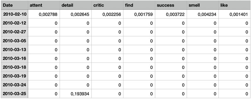
Sammanfattning
Syftet med denna studie är att analysera om det finns några specifika egenskaper i
de tweets publicerade av Donald Trump som har en korrelation med volatiliteten på
aktiemarknaden. Om egenskaper kring president Trumps tweets visar ett samband
med volatiliteten är målet att hitta en delmängd av regressorer med för att beskriva
sambandet med så hög signifikans som möjligt. Innehållet i tweets har varit i fokus
använts som regressorer.

Metoden som har använts är en multipel linjär regression med tweet och volatilitetsdata
som sträcker sig från 2010 till 2020. Som ett mått på volatilitet har Cboe VIX använts,
och regressorerna i modellen har fokuserat på innehållet i tweets där TF-IDF har använts
för att transformera ord till numeriska värden.

Resultaten från studien visar att de valda regressorerna uppvisar en liten men sig-
nifikant korrelation med en justerad R 2 = 0,4501 mellan Trumps tweets och marknadens
volatilitet. Resultaten inkluderar 78 ord som de när en är en del av president Trumps
tweets visar en signifikant korrelation till volatiliteten på börsen. Börsen är ett stort och
komplext system av många okända, som försvårar processen att förenkla och kvantifiera
data från endast en källa till en regressionsmodell med hög förutsägbarhet.

                                               3
Contents
1 Introduction 6
1.1 Background . . . . . . . . . . . . . . . . . . . . . . . . . . . . . . . . . . . . . . . . . 6
1.2 Purpose and Problem Statement . . . . . . . . . . . . . . . . . . . . . . . . . . . . . 6
1.3 Earlier research . . . . . . . . . . . . . . . . . . . . . . . . . . . . . . . . . . . . . . . 7
1.3.1 Volfefe Index . . . . . . . . . . . . . . . . . . . . . . . . . . . . . . . . . . . . 7
1.3.2 Stock Price Expectations and Stock Trading . . . . . . . . . . . . . . . . . . 8
1.3.3 Twitter mood predicts the stock market . . . . . . . . . . . . . . . . . . . . . 8
2 Economical Theory of the Study 10
2.1 The financial market . . . . . . . . . . . . . . . . . . . . . . . . . . . . . . . . . . . . 10
2.1.1 The efficient market hypothesis . . . . . . . . . . . . . . . . . . . . . . . . . . 10
2.1.2 The stock market . . . . . . . . . . . . . . . . . . . . . . . . . . . . . . . . . . 10
2.1.3 New’s impact on the financial market . . . . . . . . . . . . . . . . . . . . . . 11
2.1.4 Volatility and Cboe VIX Index . . . . . . . . . . . . . . . . . . . . . . . . . . 12
2.2 Twitter and Sentiment Analysis . . . . . . . . . . . . . . . . . . . . . . . . . . . . . . 13
3 Mathematical Theory of the Study 14
3.1 Multiple Linear Regression . . . . . . . . . . . . . . . . . . . . . . . . . . . . . . . . 14
3.1.1 Assumptions of the linear regression model . . . . . . . . . . . . . . . . . . . 14
3.1.2 Ordinary Least Squares estimation . . . . . . . . . . . . . . . . . . . . . . . . 15
3.1.3 Indicator variables . . . . . . . . . . . . . . . . . . . . . . . . . . . . . . . . . 16
3.1.4 Residual Analysis . . . . . . . . . . . . . . . . . . . . . . . . . . . . . . . . . . 16
3.2 Model assessment and verification . . . . . . . . . . . . . . . . . . . . . . . . . . . . 19
3.2.1 Leveraged and Influential points . . . . . . . . . . . . . . . . . . . . . . . . . 19
3.2.2 Multicollinearity . . . . . . . . . . . . . . . . . . . . . . . . . . . . . . . . . . 20
3.2.3 Methods for dealing with multicollinearity . . . . . . . . . . . . . . . . . . . . 20
3.2.4 Variable Selection . . . . . . . . . . . . . . . . . . . . . . . . . . . . . . . . . 21
3.2.5 Mallows Cp . . . . . . . . . . . . . . . . . . . . . . . . . . . . . . . . . . . . . 22
3.3 Quantitative Selection . . . . . . . . . . . . . . . . . . . . . . . . . . . . . . . . . . . 23
3.3.1 Selection using TF-IDF . . . . . . . . . . . . . . . . . . . . . . . . . . . . . . 23
3.3.2 Stemming . . . . . . . . . . . . . . . . . . . . . . . . . . . . . . . . . . . . . . 24
3.4 Transformation . . . . . . . . . . . . . . . . . . . . . . . . . . . . . . . . . . . . . . . 24
3.4.1 Box-Cox Transformation . . . . . . . . . . . . . . . . . . . . . . . . . . . . . . 24
4 Methodology 26
44.1 Data Gathering . . . . . . . . . . . . . . . . . . . . . . . . . . . . . . . . . . . . . . . 26
4.2 General transformation of data points . . . . . . . . . . . . . . . . . . . . . . . . . . 27
4.2.1 Transformation of Volatility . . . . . . . . . . . . . . . . . . . . . . . . . . . . 27
4.2.2 Transformation of dates . . . . . . . . . . . . . . . . . . . . . . . . . . . . . . 29
4.3 Initial models . . . . . . . . . . . . . . . . . . . . . . . . . . . . . . . . . . . . . . . . 29
4.3.1 Model 1 - statistics of tweets . . . . . . . . . . . . . . . . . . . . . . . . . . . 29
4.3.2 Model 2 - Words from Volfefe Index . . . . . . . . . . . . . . . . . . . . . . . 29
4.4 Regression Model . . . . . . . . . . . . . . . . . . . . . . . . . . . . . . . . . . . . . . 29
4.4.1 Data selection using TF-IDF . . . . . . . . . . . . . . . . . . . . . . . . . . . 30
4.4.2 Variable selection using Forward Selection . . . . . . . . . . . . . . . . . . . . 31
4.4.3 Regression . . . . . . . . . . . . . . . . . . . . . . . . . . . . . . . . . . . . . . 32
5 Results 33
5.1 Findings . . . . . . . . . . . . . . . . . . . . . . . . . . . . . . . . . . . . . . . . . . . 33
5.1.1 Interpretation . . . . . . . . . . . . . . . . . . . . . . . . . . . . . . . . . . . . 34
5.1.2 Top regressors . . . . . . . . . . . . . . . . . . . . . . . . . . . . . . . . . . . 35
5.2 Residual analysis . . . . . . . . . . . . . . . . . . . . . . . . . . . . . . . . . . . . . . 36
6 Discussion 41
6.1 Analysis of results . . . . . . . . . . . . . . . . . . . . . . . . . . . . . . . . . . . . . 41
6.2 Limitations . . . . . . . . . . . . . . . . . . . . . . . . . . . . . . . . . . . . . . . . . 42
6.3 Conclusion . . . . . . . . . . . . . . . . . . . . . . . . . . . . . . . . . . . . . . . . . 42
6.4 Further studies . . . . . . . . . . . . . . . . . . . . . . . . . . . . . . . . . . . . . . . 43
51 Introduction
1.1 Background
On June 16 in 2015, Donald Trump, a controversial and not unknown figure, at least in the United
States announced his intention to run for president of the United States of America as the republican
party’s candidate. The day before, Donald Trump’s account @realdonaldtrump had just under three
million followers on the social media platform Twitter, reading the twenty-three-thousand tweets he
had posted, not including retweets. By the start of 2020 his audience had reached sixty-eight million
accounts and his tweet legacy amounted to forty-one thousand tweets, again not counting retweets.
During this period Donald Trump has transitioned from being a famous person, predominantly
in the United States to becoming a household name worldwide. Soon ending his first period of
presidency and just putting his reelection campaign into gear with four more years in the White
House as his target, his twitter account continues to deliver daily tweets and replies. This form of
direct communication from one the world’s truly elite politicians is unprecedented.
Financial markets have always had a flavour of speculation to it as the cycle of boom, bust, rinse
repeat that keeps on iterating ever since the seventeenth century Tulip mania.[1] Motives of these
speculative moves are hard to formulate explicitly, someone able to do this would surely be able to
retire rather quickly. That political decisions play its part to some degree is something that most, if
not all, would agree on. Therefore, it is of interest to investigate the connection between president
Trump’s tweets about his work and the financial market, this will in this thesis be done using a
multiple regression analysis.
The response of Trump’s tweeting in the market will be measured with volatility. Volatility in the
financial market is of high interest as it is used in pricing derivatives and therefore play a great part
in how financial markets move in the short-to-medium time span. For this thesis the daily closing
price of the VIX index will be used.
1.2 Purpose and Problem Statement
The main purpose of this thesis is to investigate whether @realdonaldrump tweets does have an
impact on market volatility, and if so, how much and in what way? This connection will be
examined using a multiple linear regression model, with the characteristics of the tweets of a day
as the regressors and the day close for the VIX that day as response variable.
However, we must first understand that president Trump tweets multiple times almost every day,
and that very few of his tweets can be considered to influence market movements. Trumps tweets
6vary considerably in content, which is a problem when performing the regression. Tweets concerning
trade and monetary policy, that are more likely to affect the market are prone to drown in the noise
of misspelled and self-praising tweets. Therefore, this thesis will first deal with a selection of tweets
in order to determine and sort out which tweets to include in the regression. Further, a connection
between the tweets of significance and the market volatility will be quantified using a multiple linear
regression.
This paper and its findings might be of interest to a large variety of people, including the gen-
eral public and international traders investing in markets worldwide. Although this analysis will
be based on the American markets historical evidence implies that there to a varying degree ex-
ists a correlation between the market returns around the world.[2] Specifically the findings given
the methods used to could be of interest for traders deploying quantitative trading models where
volatility could determine size, timing and risk in potential trades.
Traditional model assessment and verification techniques used with regression such as analysis of
residuals and multicollinearity will be utilized. Also, a regressor of whether Donald Trump was or
was not president at the time of publishing his tweet will be implemented in the model to investigate
if the impact of Trump’s tweets before and after his presidency vary.
An important demarcation to note is that the research is limited to the effect of Donald Trumps
tweets on the market volatility on the same day of the tweet. The ambitions are not that the
findings will be able to explain market volatility fully, rather to examine which parameters of
Donald Trump’s tweets correlate and possibly impact market volatility.
1.3 Earlier research
1.3.1 Volfefe Index
The interest for President Trumps controversial behavior in Social Media have been covered in
many different angles. In September of 2019, the bank JP.Morgan Chase created a index called the
Volfefe Index, based on President Trumps Tweets.[4]
The Volfefe index was created to predict movements in treasury bonds, and in order to do this
JP Morgan had to build an algorithm for assessing tweets. To do this, every tweet’s impact was
categorised as significant or non-significant. Significant tweets were those that were followed by move
of ±0.25 basis points in 10 year Treasury yields after 5 minutes of trading from the publication of
the tweet.
Those words are, in order of decreasing significance.
71. China 6. Dollars 11. President 16. Years
2. Billion 7. Tariffs 12. Congressman 17. Farmers
3. Products 8. Country 13. People 18. Going
4. Democrats 9. Muller 14. Korea 19. Trade
5. Great 10. Border 15. Party 20. Never
This research and its findings show that there, on a small time frame exists a correlation between
Donald Trump’s Tweets and the financial market. Performing this classification of tweets is outside
the scope of this project and will not be attempted. However, the 20 most influential words for
market moving tweet shared in the article by JP Morgan will be used.
1.3.2 Stock Price Expectations and Stock Trading
In a study from 2012 researchers from RAND published a paper for the National Bureau of Economic
Research investigating stock price expectations in relations to market events. The findings from the
paper suggests that on average, subjective expectations of stock market behavior depend on stock
price changes, meaning that past performance will influence the future expectations on a stock.
Moreover, stock trading responds to changes in expectations in a delayed manner i.e. that stock
operators execute trades now even if the change in expectations occurred several ago. Implying
that news impact the market also after the time of punishment by building subjective momentum
but that the initial reaction to an event is of importance. Further the paper also discusses and
concludes the vast complexity behind market reactions and summarizes that we still don’t fully
understand how expectation on events are translated into action. [5]
1.3.3 Twitter mood predicts the stock market
Behavioral economics tells us that sentiment profoundly can influence decision-making and in-
dividual behavior. In a paper form 2011 researchers from Indiana University and University of
Manchester investigate whether this can be applied to in a larger scale that is, can societies have
states of mood that affect collective decision making? In the paper the researchers use twitter as a
data base of sentiment in society. More specifically the paper investigates whether measurements of
collective mood states derived from large-scale Twitter feeds are correlated to the value of the Dow
Jones Industrial Average (DJIA). This is done using OpinionFinder and Google-Profile of Mood
States (GPOMS). The results from the study indicate that predictions of the DJIA significantly
can be improved by including some specific public mood dimensions. The model presented in the
paper is based Self-Organizing Fuzzy Neural Network and found an accuracy of 86.7% in predicting
8the daily up and down changes in the closing values of the DJIA. Which compared to methods not
including the sentiment model reduces the Mean Average Percentage Error by over 6%.[6]
9Theoretical framework
2 Economical Theory of the Study
2.1 The financial market
2.1.1 The efficient market hypothesis
The efficient market hypothesis (EMH) made famous by Eugene Fama in the 1970s is theoretical
concept used to model financial markets, EMH puts certain demands on a market and the pricing
of securities listed on a market. A financial market is said to be efficient if the prices of securities
on the market fully reflect all available information at the time. By definition, the market is said to
be efficient to a set of information, if that information when raveled to all participants at the same
time would leave security prices unchanged. Having an efficient market with respect to some set of
information, φ, implies that there exists no opportunities of arbitrage and that it is impossible to
make economic profit trading on the already known information φ.[7]
2.1.2 The stock market
A stock market is a platform were buyers and sellers of stocks can meet and trade stocks. Each stock,
also known as a share, traded on a stock market represents a piece of ownership in the company
associated with the share. It is common to associate the term stock market to big companies listed
on big and well-known stock exchanges such as the New York Stock Exchange, NASDAQ or Dow
Jones. However, in 2020 there exists heaps of other exchanges that facilitate the same function,
but for other markets.
Historically stock markets were physical places were people met and came to an agreement on the
price and number of shares. This way of selling and buying stocks are today outdated and instead
almost all transactions occur via some form of digital platform. Different stocks trade on different
stock markets. This division is partly due to practicality, addressing the implications of different
time-zones and currencies around the world. However, there are also other factors that divide stocks
into different markets, e.g. market value. Some stock exchanges only trade publicly listed shares,
while other stock exchanges may also include securities that are privately traded. Exchanges are
not only for equities but may also list other securities for instance bonds or derivatives.[8]
The price change or movement of a stock is function of supply and demand. Depending on the
relative share of buyers and sellers the price is prone to fluctuate, and in a scenario where the
numbers of sellers exceed the number of buyers the price will decrease until the price becomes low
10enough to encourage buyers and thereby increasing the demand. The current price per share is a
function of all the current stock owners view on the company and the company’s future potential.
The difficulty of a stock market is clearly to predict price movement, since present and historical
data usually does not suffice to make accurate future projections. When predicting future prices,
one must take every person’s sentiment of the company into calculation. Because of the complexity
of this estimation future share prices are often seen as unattainable.[9]
From theoretical and empirical studies it is evident that the stock market has played a significant
role within both the advanced economy and the emerging market.[10] The stock market sentiment is
in a way a reflection of the larger economical sentiment in society. Government controlling policy’s,
professional and recreational investors, companies and media all playing their own role the stock
market. All these institutions are ultimately controlled by humans which are known to not always
act rationally. The mood on a market participant at a given point in time is referred to as Market
psychology. Emotions, including, greed, fear, expectations, and circumstances are all factors that
can contribute to market psychology at any time. As early as 1936 periodic John Maynard Keynes
described how of these sentiments in society can trigger periods of “risk-on” and risk-off”. [11]
Something that conventional financial theory mainly EMH fails to explain the emotion involved
in investing, and how this contribute to irrational behavior. In other words, theories of market
psychology are in conflict with the belief that markets are rational when they in reality never fully
are. This aspect of market psychology further adds to the complexity of predicting individual stocks
and markets performance based on fundamental facts.[12]
2.1.3 New’s impact on the financial market
The stock market is driven by and relies on new information to be unveiled. As part of EMH the
expected news is priced into the price of a stock or an index, while unexpected news is not. Stock
price movement depends on the constant change in supply and demand, making this relationship
is highly sensitive to the news of the moment. That said the anticipation of an event might be
already price in the expected event even before it’s published. On the other hand unexpected news
disclaiming something new and not priced in must first be interpreted, making chasing the news a
tricky strategy for trading.[13]
Financial markets never rest and constantly react to new information, making isolating which event
resulted in which price movement even more difficult. Generally indicators of general economic
news are found to be better than firm specific news when predicting price changes on the stock
market.[14]
Nevertheless, in a study from early 2017 not long after Trump’s presidential inauguration, re-
11searchers from Harvard and the university of Zurich published a paper trying to model asset price
responses to unexpected news in and around the election. In the morning of election day Donald
Trump was a fairly unlikely winner in the election, with betting services pricing bets with the
chance of Trump being elected to between 18-27 %. When Trump to a lot of people’s surprise
won the election, markets reacted quickly. In the paper the model for price Pn and return Rn are
modeled around the presidential election of 2016 but in theory the model can be applied to all
events with expectations on outcome. Given two outcomes X and Y with probabilities πX and πY
and respectively the current price before the event is given by
Pn = πX Pn,X + πY Pn,Y
Where PX and PY are the expected price given outcome X or Y. The expected return of given
outcome X then becomes
Pn,X − Pn
Rn =
Pn
Clearly a straightforward model including expectations and the outcome of an event. Using this
model, the researchers found that the individual stock price reactions to the election reflect the
unexpected change in investor expectations on economic growth, taxes, and trade policy. More
specifically, the market reacted quickly to the expected consequences of the election for US growth
and tax policy while, it took the market longer to incorporate the consequences of shifts in trade
policy. By evaluating the impacts of different news under a ten-day period after the election the
researchers found that one-day response varied between about 30-80% of their ten-day response.
Implying that the stock market reacts differently to different events and headlines, sometimes the
implications of news are straightforward to interpret while other times the effects of a headline is
more cumbersome to asses.[15]
2.1.4 Volatility and Cboe VIX Index
Volatility in a stock market measures the frequency and magnitude of price changes, both for
movements up and down. This applies to all traded financial instruments during a certain period
of time. The more dramatic the price fluctuation in that instrument, the larger the volatility. The
volatility is defined and measured either using historical prices, called realized volatility or as a
measurement of implied volatility by the use of options prices.[16]
The VIX, which stands for Volatility Index, is an index introduced by Chicago Board Options Ex-
change in 1993 and tries to capture the 30-day implied volatility of the underlying equity index. The
VIX uses the later and is therefore a measurement expected future volatility.[17] Cboe continuously
updates the VIX index values during trading hours. The VIX measures the implicit volatility for
12the index SP 500, which is one of the most common equity indices, that many consider to be one
of the best representations of the U.S. stock market. The VIX can be seen as a leading indicator
of investor attitudes and market volatility relating to the listed options upon which the index is
based.[18]
There is a phenomenon called volatility asymmetry which refers to the volatility being higher in
down markets than in up markets.[19] This means that volatility generally is low during longer
period of economic growth and, high during economic recessions. As a result, trading volatility
either through options or special derivatives can be used as a hedge against a downturn in the stock
market.
2.2 Twitter and Sentiment Analysis
Twitter was founded in 2006 and is one of the first social media platforms launched that still ex-
isting in 2020. The platform was launched in San Francisco, California and is now an international
microblogging and social networking service. On twitter all users can post and interact with short
statements or messages known as ”tweets”. The platform is also open for unregistered users with
the restriction being that unregistered users are limited to reading. Originally, tweets were re-
stricted to a maximum of 140 characters but in November 2017 this restriction increased to 280
characters. Twitter is accessible on both its website interface and on its mobile-device application
software.[20]
The growth of social media and social networking sites have been exponential in the past decade
for platforms such as Twitter and Facebook. This widespread phenomenon of social media raises
the possibility to track the preferences of citizens in an unprecedented manner. At the end of
2019 twitter averaged 152 million daily users.[21] The opinions and flow of information spreading
instantaneously on Twitter represents a valuable source of data that can be useful for a general
sentiment of topics.[22] This source of data comes with a complexity of analyzing emotions on social
media is due to non-standard linguistics, intensive use of slang, emojis and incorrect grammar.
Aspects that people have no problem understanding but nevertheless is troublesome for models to
interpret. Another concern is that the results of sentiment analysis on social medias such as twitter
assumes that the findings are representative for the entire population. [23] Something that might
not always be true since not everyone is connected to social media.
133 Mathematical Theory of the Study
This part will walk the reader through the more rigorous mathematical aspects of the study. Unless
otherwise stated the theory found in section 3 is extracted from Montgomery, D.C., Peck, E.A. and
Vining, G.G. (2012). [24]
3.1 Multiple Linear Regression
The hypothesis is that the the volatility on a daily basis can be explained by using a multiple linear
regression using the measurements supplied in the data set. As presented in the following linear
model for predicting the VIX index
y = β0 + β1 x1 + β2 x2 + β3 x3 + ... + βk xk +
The interpretation of this formula is that xi is the measurement of a tewwt and the goal is to find
the corresponding coefficient, βi , to be inserted into the model in order to produce the best estimate
the VIX value, here represented by y. With n observations and k covariates the model in matrix
notations is described as follows
y = Xβ +
where
β0
y1 1 x11 ··· x1k β ε1
1
y2 1 x21 ··· x2k ε2
β2 ,
y=
.. ,
X=
.. .. .. ..
,β = ε=
.. .
. . . . . .. .
.
yn 1 xn1 ··· xnk εn
βk
Here βi explains by how much the VIX is expected to change by every unit change in the measure-
ment, xi , and β0 is the intercept for the model.
3.1.1 Assumptions of the linear regression model
In the study of regression analysis major assumptions are stated. In order for the regression model to
be valid these assumptions must be proved to be true. Otherwise model inadequacies are inevitable.
The assumptions are
141. The relationship between the response variable y and the regressors x is approximately linear.
2. Error term has mean µ = 0 and constant variance = σ 2 .
3. Errors are uncorrelated. i.e. Corr(i , j ) = 0,
4. The observation of y is fixed in repeated samples. Meaning that resampling with the same
independent variable values is possible.
5. The number of observations, n is larger than the number of regressors k. Also there are no
exact linear relationships between the xi ’s.
When evaluating these conditions residual analysis is a very useful method for diagnosing violations
of the basic regression assumptions, this will be further explained later on in the study.
3.1.2 Ordinary Least Squares estimation
The values of β will be estimated using linerar model lm() function in R which utilises the ordinary
least square method and minimizes the sum of squares of the residuals. This means that the
estimation of β is given by a solution to the normal equations where the residual is defined as
e = y − Xβ
Minimizing the sum of suqares of the residuals (SSRes = e0 e) where the objective function S is
given by
β̂ = arg min S(β)
β
can be written as
n p
X X 2 2
S(β) = yi − Xij βj = y − Xβ
i=1 j=1
This minimization problem has a unique solution, provided that the k columns of the matrix are
linearly independent
(X0 X)β̂ = X0 y
Finally rewriting this we end up with the OLS estimate
β̂ = (X0 X)−1 X0 y
After the estimates of β has been produced these have to be evaluated further to assure congruence
with the assumptions relating to theory on quality of results.
153.1.3 Indicator variables
Unlike other regressor variables that have a quantitative value, the indicator variables or dummy
variables are instead qualitative variables. Since they have no natural numeric value they will in
the regression model be represented via levels either 1 or 0 assigned to them. In this study the
indicator variable is Donald trumps occupation. This indicator variables is divided in to civilian
(0) or president (1).
3.1.4 Residual Analysis
The key assumption which constitutes as the backbone of the whole project is that between VIX
and the regressors there are at least a reasonable linear relationship. By examining the produced
residual through various standardised tests and measurement, there is a higher chance of detecting
model in-adequacy.
Normal residuals
Normal residuals are defined as the difference between the observed value yi and the fitted value of
the model ŷi .
ei = yi − ŷi
The residual is interpreted as the deviation between the model and the actual data, making plotting
the residual an effective method for quickly detecting violation of model assumptions. In the best
of worlds where the model is effective the sum of all residuals should be zero and their distribution
be of the Gaussian type. In the case where this is not the case something with the model is flawed
and examining the residual will give important clues to what is wrong.
The residuals have zero mean, E(e) and their approximate average variance can be estimated
using the residual sum of squares, which has n − k degrees of freedom associated with it since k
parameters are estimated in the regression model. An estimation of the variance residuals is given
by the residual mean square M SRes
Pn 2
i=1 (ŷi − ȳ) SSres
= = M Sres
n−k n−k
16Scaled Residuals
Scaled residuals are obtained by transforming the normal residuals. The purpose of scaling is
to make residuals comparable with both each other and residuals from other models. These new
residuals can offer further clues whether something is wrong with the model and how it could benefit
from modifications. In order to understand the notations in the transformation of residuals in the
following part we will now introduce some concepts.
The total sum of squares SST is partitioned into a sum of squares due to regression, SSR , and a
residual sum of squares, SSRes .
SST = SSR + SSRes
Pn 2 Pn 2
Where the terms are defines as follows, SST = i=1 (yi − ȳ) , SSR = i=1 (ŷi − ȳ) and
Pn Pn
SSRes = i=1 (yi − yˆi )2 = i=1 (ei )2 = e0 e.
Standardized Residuals
By normalising the residuals so that they can be estimated by a Gaussian distribution with mean
equal to zero and variance of approximately one unit. This modified residual makes it easier to
analyse as the residual can be compared with other standardised residuals. As a rule of thumb a
value of di > 3 is an indication of a possible outlier. The estimation is given by
ei
di = √
M SRes
Where M SRes is an unbiased estimator of σ 2 .
Studentized Residuals
Studentized residuals builds on the standardized residuals that were obtained by nomalizing using
an estimate of variance with M SRes . To calculate studentized residuals the scaling is based of the
exact standard deviation of every i :th observation. This is calculated by dividing ei with the exact
standard deviation of the given observation i.
Writing the residual by use of the hat matrix H = X(X 0 X)−1 X 0 gives
e = (I − H))y
which through substitution in
y = Xβ +
17gives the following
e = (I − H)
Showing that the they are the same transformations of y as of . Variance of the error, is given
by Var() = σ 2 I and since I − H is symmetric and idempotent the residuals covariance matrix
is
Var(e) = Var[(I − H)] = (I − H)Var()(I − H)0 = σ 2 (I − H)
With the variance of each residual given by the covariance matrix according to
Var(ei ) = σ 2 (1 − hii )
Where hii is an element in the hat-matrix H.
Using the found variance of ei we have that the studentized residual is calculated by
ei
ri = p
M SRes (1 − hii )
The takeaway from the above formulas is that in general a xi closer to the center has a larger
variation and thus model assumptions are more probable to be challenged further out towards the
edges and that if everything about the model is sound the residual will have the variance = 1. It
could also be of use to know that as n goes to infinity, studentized residuals usually converge with
standardised residuals. As in most cases with residuals, one lonely point far away from the rest
may be influential on the whole fit. These points should be further analysed.
R-Studentized Residuals
When constructing R-Studentized residuals the variance is estimated by calculating Si2 , where i is
the an observation removed from the estimation. This is done to examine how single datapoints
influence the results, much as later described in the PRESS Residuals-section. The formula for
calculating Si2 is
(n − p)M SRes − e2i /(1 − hii )
Si2 =
n−k−1
This estimate of σ 2 is then used to calculate the R-student according to:
ei
ti = p 2
, i = 1, ..., n
Si (1 − hii )
An observation i that gives a R-studentized residual wich differs greatly from the result obtained
from estimating σ 2 using M SRes indicates that the observation, i, is an influential point.
18PRESS Residuals
PRESS, Prediction Error Sum of Squares, is another method to examine the influence of specified
observation, i, in the set. It is produced by calculating the error sum of squares from for every
observation except i. The PRESS residual is defined as
ei
e(i) = p , i = 1, ..., n
(1 − hii )
Where hii , that is the elements of the hat matrix H is large so will the PRESS residuals also be.
If this sum greatly differs from the value obtained from the whole set and the sums obtained from
excluding the other observations one-by-one the isolated point, i, has an disproportional effect on
the regression and may skew the model. This means that a point that stands out in the PRESS
diagram is a point where the model fits well but an model excluding this point will have poor results
when predicting.
3.2 Model assessment and verification
3.2.1 Leveraged and Influential points
There are many forms of outliers that can be identified, and in this section we will be looking at
leveraged points and influential points. A point of high leverage is an observation with an unusual
high x-value. If this point’s y-value is in line with the rest of the regression it won’t affect the fit
of the model too much. However, if this point also has an deviating y-value, the point becomes
an influential point. Influential points have a large effect on the model, since it pulls the entire
regression towards it. Concluding, not all leverage points are influential for the fit.
When identifying these points the Hat-matrix H = X(X 0 X)−1 X is crucial. Each element of
the hat matrix hii tells us the leverage of yi and regressors xii on the optimal fitted value ŷ i . As
a general rule a point is said to be a leveraged point if the diagonal in the Hat-matrix for that
observation exceeds double the average, 2p ≯ n.
Cook’s Distance
In order to find these points of interest, a useful diagnostics tool is Cook’s Distance. Cook’s Distance
takes into account both the x-value for the observation as well as the response variable by taking
the least square value from the observation to the fit. Cook’s distance for the i :th observation is
calculated by deleting that observation and looking at the change in the model that results from
19doing so. Cook’s distance for the observation i removed can be calculated as below, where n is the
number of observations.
ri2 V ar(ŷ i ) r2 hii
Di = = i , i = 1, 2, ..., n
k V ar(ei ) k 1 − hii
Where ri it the i :th standardized reidual hii i a diagonal element of the hat matrix H. A rule of
thumb points with Di >1 is considered to be influential points.
3.2.2 Multicollinearity
Multicollinearity occurs if the regressors are almost perfectly linear. Having multicollinearity in the
data may cause different degrees of interference in the model, symptoms range from inaccuracy of
the estimation to the model being straight out misleading and wrong. Understanding the data-set
and the source of the multicollinearity is key in treating it.
3.2.3 Methods for dealing with multicollinearity
Variance Inflation Factor
Another method for detecting multicollinearity is to look at the variance inflation factor, or VIF
for short. The VIF is defined as follows,
2 −1
V IFi = Cii = (1 − Rii )
Where C = (X 0 X)−1 , R2 denotes the coefficient of determination and each observations is Cii =
−1
(1 − Rii ).
If xi is nearly linearly dependent to some subset of regressors, Cii becomes very large. A V IFi
value of 10 indicate multicollinearity which can result in poor estimations of β.
Eigenvalue Analysis
One of the most common analysis for detecting multicollinearity is to look at the eigenvalues of
X’X in our system. The easiest way to determine whether there is multicollinearity is to look at
the condition number of X’X, defined as
λmax
k=
λmin
20The common rule of thumb is that
• k = 1 implies perfectly orthogonal regressors and no multicollinearity
• k < 100 implies week multicollinearity
• 100 < k < 1000 relates to moderate to strong multicollinearity
• k > 1000 is sign of severe multicollinearity.
3.2.4 Variable Selection
A contradiction that occurs in any regression model is the problem with the number of variables.
Firstly, it would be preferred to include as many regressors as possible for the purpose of having
the largest scope of information. On the other hand, too many regressors inflate variance which
will have a negative impact on the overall performance of the model.
All Possible Regression
This method fits all the possible regression equations involving one candidate regressor, two candi-
date regressors, and so on. The optimal regression model is then selected based on some criterion,
in our case Baysian Information Criteria, Mallows Cp and adjusted R2 . This technique is rather
computational heavy and is not suited for models with many regressors. A model with k candidate
regressors result in that there are 2 k total equations to be estimated and examined. For depending
on the number of regressors in model this technique may not be possible. For models under 30
regressors this method is acceptable using the computers of 2020. For models containing more
than 30 regressors variable selection can be achieved using either forward, backward or stepwise
elimination.
Forward Selection
Forward elimination starts with a blank model solely including the interception β0 . Then the model
adds one regressor at a time in order to to find the optimal subset of regressors. The first variable is
chosen based on the largest simple correlation with the response variable. When adding the second
regressor, the method again chooses the regressor with the largest correlation to the response
variable, after adjusting for the first variable. The regressors having the highest partial correlation
will produce the largest value of F statistic for testing the significance of the regression.
21Backward Elimination
The inverse of forward selection. Starting the model with all the regressors being in the model.Then
the F statistic is evaluated for all regressors as if it was the last to enter the model. Then the model
simply removes the regressor with the smallest F statistic. Repeat.
Baysian Information Criterion
Bayesian information criterion, or BIC, is a criterion that balances the number of regressors to
the number of observations. The BIC is used for variable selection and places penalty on adding
regressors to the model. The BIC can be computed as
SSRes
BIC = n ln + k ln(n)
n
The variable k denotes the number of coefficients including the intercept and n is the number of
observations.
R2 and adjusted R2
Another way to evaluate the adequacy of the fitted model is to look at the R2 for the generated
models.
SSR
R2 =
SST
Where SST is the total sum of squares and SSR is sum of squares due to regression. However R2
dose not take the number of variables in to consideration. it never decreases when new variable is
added to the model. This is why adjusted R2 is used as a criteria instead, this takes the number of
regressors in to consideration.
2 SSR /(n − p)
Radj =1−
SST /(n − 1)
The definition of adjusted R2 for a model with n observations and k regressors.
3.2.5 Mallows Cp
Mallow’s Cp presents a variance based criterion, defined as
SSRes
Cp = − n + 2p,
σ̂ 2
22where σ̂ 2 is an estimator of the variance, e.g. M SRes . It can be shown that if the p-term is without
bias, the estimated value of the Cp equals p. When using the Cp criterion, it can be helpful to
visualize it in a plot of Cp as a function of p for each regression equation, this is exemplified in
figure 1. Models with little bias will have values of Cp that fall near the line Cp = p. While
regression equations with bias e.g. point B, are illustrated above this line. Generally, small values
of Cp are desirable. On the other hand small bias may be preferred for the sake of a simpler model,
in the case illustrated in figure 1 C can be preferred over A even tough in includes bias.
Figure 1: A Cp plot example
3.3 Quantitative Selection
3.3.1 Selection using TF-IDF
TF-IDF is a quantitative measure reflecting the importance of a single word in a sentence or
collection of words. [25] TF-IDF is defined as the product of two terms, term frequency (TF) and
inverse document frequency (IDF).
The term frequency is used to measure how frequent a word is in the given document. TF treats
the problem of documents having different total word counts. To compensate for documents having
unequal lengths the TF takes the occurrence of the specific word and divides it with the total word
count.
Occurrences of word X in document Y
TF =
Word count in document Y
23For the second part, the inverse document frequency attempts to distinguish relevant and non-
relevant terms by observing whether the term is common or rare across all documents. The IDF
assigns lower values to common words and assigns larger values for the words that are rare. This is
done by the logarithmically scaled inverse fraction of the documents that contain the word.
Number of documents
IDF = log
Documents that contain the term X
And as previously stated the TF-IDF is simply the frequency multiplied by the inverse document
frequency. Calculating the TF-IDF for all terms in a corpus will assign a numeric value of sig-
nificance to each word in each document. This value represents how important a specific word is
to the collection of documents. The higher the TF-IDF value, the greater the importance of the
word.
However, the method of TF-IDF are not without limitations. For instance, it does not retain the
semantic context of words in the initial text. Moreover TF-IDF is unaware of synonyms or even
plural form of words. [26] This can be handled trough the process of stemming.
3.3.2 Stemming
The process of stemming is in morphology and information retrieval of reducing words to their core
form. For instance the words consultant, consultants, consultancy, consulting are all reduced to
their stem-form, that is consult. The word do not need to be an inflection of a word, it is enough
that related words map to the same stem. [27] Even if the word in itself is not a valid root. All this
is accomplished through algorithms. The process is implanted in our every day life, for instance
many search engines treat word of the same stem as the same as synonyms as a way to expand the
query.[28]
3.4 Transformation
3.4.1 Box-Cox Transformation
Box-Cox is used in order to investigate whether the data set requires transformation to correct for
non-constant variance or non-normality. If the model needs transformation this can be done by
utilising the method presented by, and named after, Box and Cox. The method deploys the fact
that y λ can be used to adjust for non-normality or non-constant variance. Lambda is a constant
estimated by maximizing
241
L(λ) = − n ln (SSRes (λ))
2
Plotting L(λ) and drawing vertical lines marking the the horizontal lines L(λ̂) − 21 χ2α,1 on the y-
axis, two intersections are found. χα,1 is the upper α percentage point of the chi-square distribution
with one degree of freedom. Mening that for α = 0.05 the x-values of the vertical lines indicate the
border of a 95 per cent CI. If 1 is inside of this CI it implies that no transformation is needed. In
other cases the recommended transform is.
λ
yi − 1 if λ 6= 0,
(λ)
yi = λ
ln yi if λ = 0,
This is the one-parameter Box–Cox transformations that will be used to transform data. The
exact value of λ is within the 95 per cent CI confidence interval but not exactly known. The
transformation process becomes because of this one of trail and error and the method can be
repeated if one transformation was unsatisfying.
254 Methodology
In this section the iterative process of finding the final model is described. Before obtaining the
final model and evaluating it two initial models were tested and discarded. For the model building
the majority of the time was spent on sorting and selecting different aspects of the tweets. In order
to understand the selection and transformation of the data, the two data sets used are described
below.
4.1 Data Gathering
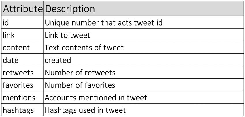
Two data sets that were used to carry out this analysis are firstly, the regressors containing all of
Trump’s tweets with a date- and time stamp, as well as the number of favourites and retweets.
The data of President Trumps Tweets were found as an open source csv-file at Kaggle.com.[29]
This data set contains all of Donald Trump’s tweets from his very first tweet the May 4th 2009 all
the way to January 20th 2020, summing to 41 060 unique tweets. This data do not include any
retweets.
Figure 2: Tweet attributes and their descriptions
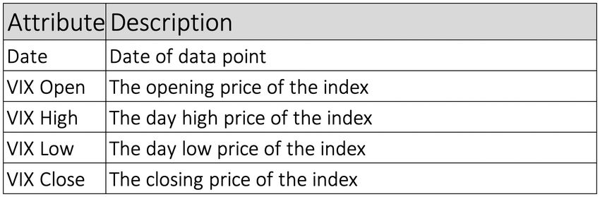
The second data set needed is that of the volatility of the stock market. Here there are plenty of
options and a wealth of different data. The Cboe Volatility Index ($VIX) will be used. There are
two reasons, one the index measuring implicit volatility and has the advantage of having unweighted
data. This data is found directly on Cboe’s website.[30]
26Figure 3: VIX attributes and their descriptions
In the following analysis a transformed value of VIX Close will be utilized.
4.2 General transformation of data points
4.2.1 Transformation of Volatility
When performing the regression analysis it is key that the response variable has a normally dis-
tribution. Below is a graph showing the VIX index with a mean value of 18.34, a maximum and
minimum value of 82.69 and 9.14 respectively during the last 10 years.
Figure 4: VIX index historical prices
As can be seen in figure 5 the distribution of the VIX price clearly is not normally distributed. This
can be seen in the histogram of VIX Close prices below.
27Figure 5: VIX index histogram Figure 6: Transformed VIX index histogram
Box Cox transformation was used to transform the VIX data. This resulted in a transformation
of.
VIXtransformed = log(VIX)−2
Observing figure 6, the new histogram of transformed data understandably normalised the VIX
closing prices. The transformation is further strengthened by the Box-Cox intervals in figure 7,
were one can ovserve λ = 1 within the confidence interval of 95 per cent. Indicating that no further
transformation of the response variable is necessary.
Figure 7: BoxCox parameter λ with the 95 % CI shown.
284.2.2 Transformation of dates
The data of tweets include both date and an exact time of when the tweet was published. Since the
VIX data set only has day resolution, this had to be taken in to consideration. The closing price
for the VIX data set is set at 16:00 eastern time, while all tweets sent after 16:00 are regarded as if
they belong to the next trading day. This is done with the argument that tweets sent after closing
hours simply are unable to impact the volatility the same day.
4.3 Initial models
4.3.1 Model 1 - statistics of tweets
The first thing that was tried was building a model with only the quantitative data from given by
the tweets, disregarding the content of the tweets. In order to achieve this the statistics from each
day was summed. The regressors for this model are.
• Number of retweets for tweets posted that day
• Number of favorites for tweets posted that day
• Length of tweet in terms of characters
• Number of tweets that day
This model presented an adjusted R2 of 0.024. Clearly using the statistics of the tweets will not
tell us much about volatility.
4.3.2 Model 2 - Words from Volfefe Index
The second model constructed took the words of importance stated in the Volfefe study in to
consideration. This model simply sorted out all the tweets that did not contain any of the 20 key
words given in the Volfefe study by JP.Morgan. This model did not perform well with an adjusted
R2 of 0.072. The main problem identified with this approach was that with only 20 words to many
days when none of these words where tweeted gave no input to the model. From this attempt the
key takeaway was that as many days as possible need to be considered, and tha using only 20 words
left to many days and tweets out of the model.
4.4 Regression Model
Learning form the first two attempts of models the final model focuses on selected words mentioned
per day in the tweets of Donald Trump.
294.4.1 Data selection using TF-IDF
The first step was to gather all words tweeted per day in a bag of words for this day. This bag of
words will act as a representation of that day. In this step of the process we perform the first step
in clearing the data by removing puncts, hyphens and other symbols. This operation is justified
by arguing that symbols by them self are without meaning, unless there is context. By the same
logic all stop words are removed. Stop words are words, that just like symbols are meaningless
without context. Examples of stop words are, whom, this, that, these, am, is, in total 175 words
are considered and stripped using the package quanteda in R.[31]
By creating a matrix with days represented as rows and each word represented as a column, we have
a matrix of 3 116 days by 38 516 words. Were each word is represented by an integer indicating
how many times that word appeared in his tweets on that day. With the words set out to act as
regressors later it is easy to understand that the number of words further need to be reduced.
Secondly the process of stemming is applied. After removing stop words and applying stemming
to all words remaining the number of unique words was reduced to 31 608. Stemming also, more
importantly gathers information of the same kind. For instance, the word China will be reopened
not only by occurrences of China but also by Chinese, China’s, etc. The thought behind this is that
the words of the same stem essentially have the same meaning and refers to the same thing.
The next step is to calculate the TF-IDF of the matrix. This do not change the dimensions of the
matrix. After this calculation each word each day is represented by a a number. This number is
the TF-IDF which if the word is tweeted during the day is a decimal numeral and 0 if the word
in question don’t appear during the day. This TF-IDF number can be interpreted as, how many
times Trump tweeted that word on that day compared to the other days. In figure 6 below a small
sample of the TF-IDF data table.
30Figure 8: TF-IDF data table
Thirdly, and removing the bulk of words the appearance of words is considered. The words that do
not appear more than 25 times are stripped from the data. Arguing that it’s hard to know what
to make of these words since they appear so infrequently. Weekends when markets are closed are
also removed. This results in regressors now having the dimensions of 2 502 days by 1 706 words,
with each word being a regressor. The regressor value is represented by the words TF-IDF value
for that day.
Finally, a last regression variable was added and another one was made binary. This regressor
represents whether Donald Trump is president of not at the date of his tweet. This was represented
as a factor of two levels, 0 = civilian and 1 = president. Moreover, the regressor ’pic.twitter.com’
which represents if there was a picture attached to tweet was transformed to be binary, either one
or zero.
4.4.2 Variable selection using Forward Selection
In order to further reduce the number of regressors forward selection is used. This is done to avoid
over fitting and remove the features that don’t contribute to the performance of the model. Forward
selection was chosen over the all possible regression method of regressors, which in the case of 1707
regressors is infeasible since the algorithm have to search over 21707 features combinations. Thus,
forward selection was used, the forward selection was then evaluated using Baysian Information
Criterion, Mallows Cp and adjusted R2 . Where we would like to minimize the BIC as well as the
Cp with regards to the number of regresses, and of course maximize the adjusted R2 .
31Figure 9: BIC Figure 10: Mallows Cp Figure 11: adjusted R2
Evaluating with regards to BIC we find the optimal model to consist of 79 regressors. Mallows
Cp suggests that 392 regressors should be used in the model. Finally evaluating on adjusted R2
recommends 981 variables to be used.
These criterion’s of evaluation all recommend quite different models to be used. And there is no
easy correct answer to witch to use. Despite its popularity and being intuitive, the adjusted R2 is
not as well motivated in statistical theory as BIC, and Cp[32].
To decide which model to chose as the final one the model recommended both by BIC and Mallows
Cp was evaluated. This was done by performing the regression using the lm() command in R and
observing the p-values of individual regressors for the model. For the model of regressors selected
by BIC all p-values are close to or equal to zero.
For the model of regressors selected by Cp quite a few coefficients have large p-value which is
undesirable. More over, with many features we lose interpretability, while with less words we can
have more insights on them. Concluding, that even though a lower adj-R2 for the model selected by
Baysian Information Criterion this model will be used. The selected regressors for the final model
is stated in section 5.1 Findings.
4.4.3 Regression
At this stage a multiple linear regression was carried out using the transformed value of VIX
1/log(V IX)2 as response variable and the TF-IDF data table with the 79 words suggested by BIC
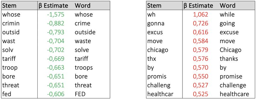
as regressors. The regression is carried out in R using the command lm().
325 Results
5.1 Findings
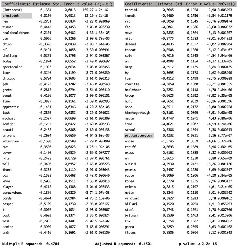
The Output from the final regression model is
Figure 12: Output from regression
33Figure 11 shows the full model of all regressors. We find the adjusted R2 = 0.4501 and the sum
of residuals to −1.553852e−18. Some of the regressor’s names will look a bit strange due to the
process of stemming, for instance the stem of leaving and leave are both included in the stem leav.
Here the regressors marked in grey ’president’ is a indicator variable and ’pic.twitter.com’ is binary.
Apart from these two exceptions all other regressors are represented by their TF-IDF value.
5.1.1 Interpretation
The β’s in the model are hard to interpret in their current state due to the transformation of
volatility. The reverse transform is given by
r
1
VIX = exp
VIXtransformed
This means that the intercept β0 which in our model has a value of 0.1334 transforms to 15.45,
which is a bit lower than the median VIX of 15.60. Another big part to this transformation is that
negative coefficients of βi contribute to a higher price of the VIX, not lower. A positive βi such as
that for ’oil’ contribute to a lower price of the VIX.
To calculate the expected VIX one would calculate the TF-IDF for the word during a day. Then
putting the values of these words into the model. For example, a day only counting one of President
Trump’s more known tweets
Why would Kim Jong-un insult me by calling me "old," when I would NEVER call him "short
and fat?" Oh well, I try so hard to be his friend - and maybe someday that will happen!
Would not contribute to the model since none of the words in the tweet is in the model. The model
would the output β0 = 0.1334, which transformed relate to a VIX of 15.45. If trump however were
to tweet,
Canada will now sell its oil to China because @BarackObama rejected Keystone. At least
China knows a good deal when they see it.
Were two key words are mentioned, oil and china. Calculating the TF-IDF values for these words
they are 0,092301 and 0,11255 respectively. Inserted in the model this gives
VIXtransformed = β0 + βpresident + βoil TF-IDFoil + βchina TF-IDFchina
With the values put in our VIXtransformed becomes equal 0,07940 to which corresponds to an estimate
of the VIX of 34,7685. Comparing this to the median value of 15.6 for the VIX during the last 10
34You can also read