Simulated wind farm wake sensitivity to configuration choices in the Weather Research and Forecasting model version 3.8.1
←
→
Page content transcription
If your browser does not render page correctly, please read the page content below
Geosci. Model Dev., 13, 2645–2662, 2020
https://doi.org/10.5194/gmd-13-2645-2020
© Author(s) 2020. This work is distributed under
the Creative Commons Attribution 4.0 License.

Simulated wind farm wake sensitivity to configuration choices in the
Weather Research and Forecasting model version 3.8.1
Jessica M. Tomaszewski1 and Julie K. Lundquist1,2
1 Department   of Atmospheric and Oceanic Sciences, University of Colorado, 311 UCB, Boulder, CO 80309, USA
2 National   Renewable Energy Laboratory, Golden, CO, USA

Correspondence: Jessica M. Tomaszewski (jessica.tomaszewski@colorado.edu)

Received: 24 October 2019 – Discussion started: 9 December 2019
Revised: 20 April 2020 – Accepted: 8 May 202 – Published: 16 June 2020

Abstract. Wakes from wind farms can extend over 50 km               newable Energy Wind Energy Technologies Office. The views ex-
downwind in stably stratified conditions. These wakes can           pressed in the article do not necessarily represent the views of the
undermine power production at downwind turbines, ad-                DOE or the U.S. Government. The U.S. Government retains and
versely impacting revenue. As such, wind farm wake im-              the publisher, by accepting the article for publication, acknowledges
pacts must be considered in wind resource assessments, espe-        that the U.S. Government retains a nonexclusive, paid-up, irrevoca-
                                                                    ble, worldwide license to publish or reproduce the published form of
cially in regions of dense wind farm development. The open-
                                                                    this work, or allow others to do so, for U.S. Government purposes.
source Weather Research and Forecasting (WRF) numerical
weather prediction model includes a wind farm parameter-
ization to estimate wind farm wake effects, but model con-          1   Introduction
figuration choices can influence the resulting predictions of
wind farm wakes. These choices include vertical resolution,         Wind energy is growing rapidly to meet increasing energy
horizontal resolution, and whether or not to include the ad-        demands with lower-carbon electricity sources. A wind tur-
dition of turbulent kinetic energy generated by the rotating        bine generates electricity by using momentum from the wind
wind turbines. Despite the sensitivity to model configuration,      to turn its blades and generator, causing a downwind wake
no clear guidance currently exists for these options. Here we       characterized by a reduction in wind speed and an increase in
compare simulated wind farm wakes produced by varying               turbulence (Lissaman, 1979). The aggregate impact of these
model configurations with meteorological observations near          individual turbine wakes can extend over 50 km downwind
a land-based wind farm in flat terrain over several diurnal         of a wind farm, particularly during stable conditions when
cycles. A WRF configuration comprised of horizontal reso-           little atmospheric convection is present to erode the wake
lutions of 3 km or 1 km paired with a vertical resolution of        (Christiansen and Hasager, 2005; Platis et al., 2018). Con-
10 m provides the most accurate representation of wind farm         sequences of these wake effects include local changes to
wake effects, such as the correct surface warming and ele-          surface fluxes that can raise surface temperatures at night
vated wind speed deficit. The inclusion of turbine-generated        caused by turbine-induced mixing of the nocturnal inversion
turbulence is also critical to produce accurate surface warm-       (Baidya Roy, 2004; Baidya Roy and Traiteur, 2010; Zhou
ing and should not be omitted.                                      et al., 2012; Rajewski et al., 2013, 2016; Smith et al., 2013;
                                                                    Siedersleben et al., 2018a) and loss of power and revenue
                                                                    for downwind wind farms operating in the wind speed deficit
                                                                    (Nygaard, 2014; Nygaard and Hansen, 2016; Nygaard and
Copyright statement. This work was authored [in part] by the Na-    Newcombe, 2018; Lundquist et al., 2018). As wind farms
tional Renewable Energy Laboratory, operated by Alliance for Sus-   continue dense development, wind farm wake impacts must
tainable Energy, LLC, for the U.S. Department of Energy (DOE)
                                                                    be considered in wind resource assessments.
under Contract No. DE-AC36-08GO28308. Funding provided by
the U.S. Department of Energy Office of Energy Efficiency and Re-

Published by Copernicus Publications on behalf of the European Geosciences Union.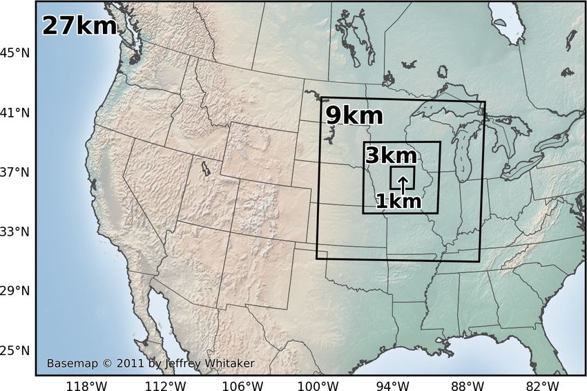
2646                                      J. M. Tomaszewski and J. K. Lundquist: WRF WFP configuration affects wakes

   Several numerical simulation tools exist to assess wind        bines in each model grid cell as a turbulence source and a
farm wake effects. Large-eddy simulations (LES) provide           momentum sink within the vertical levels of the turbine rotor
fine-scale information of near-turbine meteorological im-         disk (Fitch et al., 2012; Fitch, 2016). A fraction of the kinetic
pacts of wind turbines (Sørensen and Shen, 2002; Vermeer          energy extracted by the virtual wind turbines is converted to
et al., 2003; Calaf et al., 2010; Troldborg et al., 2010;         power, reported as an aggregate sum in each model grid cell.
Sanderse et al., 2011; Churchfield et al., 2012; Archer et al.,   The default setting of the WFP dictates that turbine-induced
2013; Aitken et al., 2014; Mirocha et al., 2014; Abkar and        turbulence generation is derived from the difference between
Porté-Agel, 2015a, b; Vanderwende et al., 2016; Marjanovic        the thrust and power coefficients, though this option can be
et al., 2017; Tomaszewski et al., 2018). Simulating the tur-      switched off to constrain turbulent kinetic energy (TKE) to
bine rotor and downstream flow with LES is useful, al-            be added only via wind shear arising from the momentum
beit computationally expensive, making realistic LES simu-        deficit in the wake of the turbine. Wind-speed-dependent
lations of entire wind farms that can span 100s of km2 unrea-     thrust coefficients specify the local wind drag on kinetic en-
sonable. Reynolds-averaged Navier–Stokes (RANS) approx-           ergy extraction as well as on power estimation. Users can
imations (Cabezón et al., 2011; Tian et al., 2014; Göçmen         modify the specifications of the parameterized turbine, such
et al., 2016; Astolfi et al., 2018; Iungo et al., 2018) and in-   as its hub height, rotor diameter, power curve, and thrust co-
dustry flow models (e.g., FLOw Redirection and Induction in       efficients, as well as its latitude and longitude location.
Steady State – FLORIS; NREL, 2019) and Wind Farm Simu-               The WRF WFP has been employed in many studies with
lator (WFSim; Boersma et al., 2016) are commonly used for         different model configurations to assess the impacts of on-
lower-cost wind farm wake investigations (Beaucage et al.,        shore and offshore wind farms (e.g., Eriksson et al., 2015;
2012). However, these models are often limited in parame-         Jimenez et al., 2015; Miller et al., 2015; Vanderwende et al.,
terizations of meteorological effects such as atmospheric sta-    2016; Vanderwende and Lundquist, 2016; Wang et al., 2019).
bility or large-scale wind patterns.                              WFP simulations have reproduced the observed localized,
   One approach to parameterizing turbines numerically in         nighttime, near-surface warming caused when wind tur-
simulations with grid spacings of kilometers or more is to        bines mix warmer air from the nocturnal inversion down to
exaggerate surface roughness to represent the local reduc-        the surface (Fitch et al., 2013; Lee and Lundquist, 2017b;
tion of wind speed of wind farm wakes (Keith et al., 2004;        Siedersleben et al., 2018a; Xia et al., 2019). Such findings
Frandsen et al., 2009; Barrie and Kirk-Davidoff, 2010; Fitch,     have prompted additional studies using the WFP to address
2015). This enhanced surface roughness approach was later         whether large-scale wind farms could alter regional climate
shown to produce erroneous predictions, including the wrong       (see Table 1 for an overview). Specific examples include
sign of surface temperature change through the diurnal cy-        Vautard et al. (2014), which used WFP simulations of fu-
cle (Fitch et al., 2013). Emeis and Frandsen (1993) pro-          ture European deployment at a 50 km horizontal resolution
posed and later refined (Emeis, 2009) an analytical wind park     and ∼ 30 m vertical resolution to find statistically significant
model that considers both momentum loss and downward              temperature signals only in winter, constrained to ±0.3 K.
momentum flux, which accounts for the spatially averaged          Conversely, Pryor et al. (2018) use the WRF WFP at a 4 km
and stability dependent momentum-extraction coefficient by        horizontal resolution and ∼ 30 m vertical resolution to find
turbines. While the Emeis model incorporates the influence        that wind farm-induced surface warming (< 0.1 K on aver-
of additional wake characteristics, it lacks consideration for    age) around wind farms in Iowa is more significant during
turbine-scale interactions between the rotor layer and the sur-   summer months. Miller and Keith (2018), using WFP simu-
face (Fitch et al., 2012; Abkar and Porté-Agel, 2015a).           lations at a 30 km horizontal resolution and 25 m vertical res-
   Alternatively, the turbine power and thrust curves can de-     olution, suggest that generating today’s United States elec-
fine the elevated momentum sink and turbulence genera-            tricity demand (which they estimate to be 0.46 TWe ) with
tion of a wind turbine. The turbine power and thrust curves       only wind power would redistribute boundary-layer heat to
give the relationship between hub-height inflow wind speed,       warm the continental United States (CONUS) surface tem-
power production, and force exerted onto the ambient air by a     peratures by 0.24 K.
specific wind turbine type. The use of these turbine specifica-      The varying WRF WFP configurations employed in previ-
tions can predict meteorological impacts of wind turbines at      ous wake studies present conflicting depictions of the impact
hub height extending down to the surface, forming the basis       of wind farm wakes, suggesting a sensitivity to model set-
for multiple wind farm parameterizations in mesoscale nu-         tings. Past studies have begun evaluating this sensitivity in
merical weather prediction models, such as the Wind Farm          the WRF WFP. Lee and Lundquist (2017a) note that a ∼12 m
Parameterization (WFP) (Fitch et al., 2012; Fitch, 2016),         vertical resolution is necessary to reproduce observed power
the Explicit Wake Parametrisation (Volker et al., 2015), the      production, while Mangara et al. (2019) find that the wake
Abkar and Porté-Agel (2015b) Parameterization, and a hy-          dynamics simulated by the WFP are more sensitive to hor-
brid wind farm parametrization (Pan and Archer, 2018).            izontal resolution than vertical resolution. Xia et al. (2019)
   The open-source WFP of the Weather Research and Fore-          find differences in the WFP solution of surface temperature
casting (WRF) model acts to collectively represent wind tur-      changes, depending on the inclusion of the turbine-generated

Geosci. Model Dev., 13, 2645–2662, 2020                                            https://doi.org/10.5194/gmd-13-2645-2020
J. M. Tomaszewski and J. K. Lundquist: WRF WFP configuration affects wakes                                                                      2647

Table 1. Overview of previous WRF WFP wake impact studies

                      Reference                              Horizontal           Vertical        Near-surface T impact due to
                                                            resolution1        resolution2        vertical redistribution of heat3
                      Fitch et al. (2013)                          1 km                15 m       increase of 0.5 K
                      Vautard et al. (2014)                       50 km                30 m       wintertime changes ±0.3 K
                      Miller and Keith (2018)                     30 km                25 m       increase of 0.24 K across CONUS
                      Pryor et al. (2018)                          4 km                30 m       increase of < 0.1 K
                      Siedersleben et al. (2018a)               1.67 km                35 m       increase of 0.4 K
                      Wang et al. (2019)                           1 km                 7m        wintertime increase of 0.2 K
                      Xia et al. (2019)                            1 km                20 m       increase of 0.3 K
                    1 Of innermost domain, if applicable. 2 Within rotor layer. 3 Within wind farm, unless otherwise specified.

TKE term. Siedersleben et al. (2020) determine that a TKE                            wende et al., 2015; Bodini et al., 2017; Sanchez Gomez and
source and a horizontal resolution on the order of 5 km or                           Lundquist, 2020).
finer are necessary to represent the impact of offshore wind                            The WINDCUBE 200S scanning lidar was positioned
farms on the stably stratified, marine atmospheric boundary                          within the northern half of the wind farm during CWEX-13,
layer. Sensitivity studies conducted for the New European                            about six rotor diameters north of the nearest turbine row.
Wind Atlas find a sensitivity to modifications to the MYNN                           The 200S lidar utilized a velocity azimuth display (VAD)
scheme in different WRF versions (Witha et al., 2019; Hah-                           scanning strategy that measured winds from ∼ 100 to 4800 m
mann et al., 2020). The MYNN scheme within WRF Ver-                                  above ground level (a.g.l.) approximately every 50 m. We use
sions 3.7.X to 3.9.X differs from 4.X most notably in the drag                       the 200S 75◦ elevation scans (Vanderwende et al., 2015) in
coefficient parameterization in the surface layer subroutine                         this study to estimate horizontal winds every 30 min to vali-
and the mixing length formulation, leading to differences in                         date the boundary-layer winds simulated by WRF.
the wind that could impact wake studies (Olson et al., 2016).                           We select 24 through 27 August of 2013 for our analysis.
While these studies give initial guidance on the sensitivity of                      During this period, a lack of major synoptic events allowed
the WFP to model settings, a greater breadth of spatial reso-                        strong nightly nocturnal low-level jets (LLJ) to occur (Van-
lution and WFP TKE sensitivity tests are needed to formulate                         derwende et al., 2015). Lee and Lundquist (2017a) found that
more confident best practice guidelines.                                             WRF performed well in capturing the timing, intensity, and
   Here we expand upon and synthesize the work of Lee and                            position of these low-level jets. Furthermore, the wind tur-
Lundquist (2017a), Mangara et al. (2019), Xia et al. (2019),                         bines operated without curtailment, and the instruments were
and Siedersleben et al. (2020) and provide guidance on opti-                         online collecting data, making this period ideal for a model
mal WRF WFP model settings for simulating wakes. Sec-                                sensitivity and performance evaluation.
tion 2 outlines the model setup and configurations tested;
Sect. 3 presents the differences in the configurations, and                          2.2     Modeling
Sects. 4 and 5 summarize our results confirming model sen-
sitivity and recommend WRF WFP modeling choices.                                     We conduct all simulations but one in our sensitivity study
                                                                                     with version 3.8.1 of the Advanced Research WRF (ARW)
                                                                                     model (Skamarock and Klemp, 2008). While model time
2     Data and methods                                                               step, vertical resolution, horizontal resolution (and thus do-
                                                                                     main size), and model version are among the model settings
2.1    Observations                                                                  varied to test sensitivity, several model options are kept con-
                                                                                     sistent across all simulations based on previous studies of this
This sensitivity analysis relies on data from the Crop Wind                          time period. The 0.7◦ ERA-Interim (ECMWF, 2009; Dee
Energy Experiment (CWEX). CWEX investigated the inter-                               et al., 2011) data set provides initial and boundary conditions
section of agriculture and wind energy within the planetary                          for all model runs, chosen for its better performance over
boundary layer (PBL) (Rajewski et al., 2013). The site was                           other reanalysis data sets (Lee and Lundquist, 2017a; Hah-
characterized by generally flat terrain and a vegetated sur-                         mann et al., 2020). Topographic data are provided at 30 s res-
face of corn and soybeans and featured an operating wind                             olution. Physics options include the Rapid Radiative Trans-
farm northeast of Ames, Iowa. In the 2013 CWEX cam-                                  fer Model (RRTM) long-wave radiation scheme (Mlawer
paign, seven surface flux stations, a radiometer, three pro-                         et al., 1997), the single-moment 5-class microphysics scheme
filing lidars, and a scanning lidar were deployed within and                         (Hong et al., 2004), land surface physics with the Noah Land
around this wind farm to explore the interaction of multiple                         Surface Model (Ek et al., 2003), Dudhia short-wave radia-
wakes in a range of atmospheric stability conditions (Vander-                        tion (Dudhia, 1989) with a 30 s time step, a surface layer

https://doi.org/10.5194/gmd-13-2645-2020                                                                      Geosci. Model Dev., 13, 2645–2662, 2020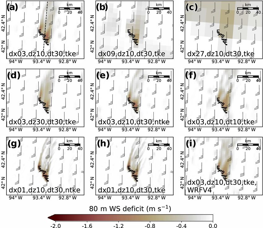
2648 J. M. Tomaszewski and J. K. Lundquist: WRF WFP configuration affects wakes
Table 2. Simulation Configurations
Identifier Horizontal Vertical Time step TKE WRF Computation time
resolution (dx) resolution (dz) (dt) option version (CPU h)∗
dx03_dz10_dt30_tke 3 km 10 m 30 s Default 3.8.1 200
dx09_dz10_dt30_tke 9 km 10 m 30 s Default 3.8.1 50
dx27_dz10_dt30_tke 27 km 10 m 30 s Default 3.8.1 12
dx03_dz30_dt30_tke 3 km 30 m 30 s Default 3.8.1 150
dx03_dz10_dt30_ntke 3 km 10 m 30 s No added TKE 3.8.1 200
dx03_dz10_dt10_tke 3 km 10 m 10 s Default 3.8.1 650
dx01_dz10_dt30_ntke 1 km 10 m 30 s No added TKE 3.8.1 630
dx01_dz10_dt30_tke 1 km 10 m 30 s Default 3.8.1 630
dx03_dz10_dt30_tke_V4 3 km 10 m 30 s Default 4.0 200
∗ Per 1 d (24 h + 12 h spinup) of simulation. Domain sizes indicated in Fig. 1.
scheme that accommodates strong changes in atmospheric For example, we test vertical resolution sensitiv-
stability (Jimenez et al., 2012), the second-order Mellor– ity by comparing the baseline configuration to the
Yamada–Nakanishi–Niino (MYNN2) PBL scheme (Nakan- dx03_dz30_dt30_tke configuration, which coarsens the ver-
ishi and Niino, 2006) without TKE advection, and the explicit tical resolution from 10 m in the baseline to 30 m (dz30) and
Kain–Fritsch cumulus parameterization (Kain, 2004) on do- reduces the number of layers intersecting the turbine rotor
mains with horizontal resolutions coarser than 3 km. layer from ∼ 7 to 3 (Fig. 2). We test sensitivity to horizontal
We simulate each 24 h day of 24 through 27 August in- resolution by separately nesting higher-resolution domains,
dividually, beginning spinup at 12:00 Coordinated Universal first using only a 27 km domain, then adding a 9 km do-
Time (UTC) on the previous day with analysis retained after main, a 3 km domain, and finally a 1 km domain (Fig. 1).
00:00 UTC. We define the wake effect by comparing a sim- Our finest domain tested is 1 km to avoid issues with the
ulation without the WFP to a simulation with the WFP, as Terra Incognita (Wyngaard, 2004; Ching et al., 2014; Zhou
in Fitch et al. (2012), Lee and Lundquist (2017a), and Red- et al., 2014; Doubrawa and Muñoz Esparza, 2020). Addition-
fern et al. (2019). We use the power and thrust curve of the ally, we test the impacts of the WFP turbine-generated TKE
1.5 MW Pennsylvania State University (PSU) generic turbine source by running two simulations with this option switched
(Schmitz, 2012) to parameterize the wind turbines, based on off (dx03_dz10_dt30_ntke and dx01_dz10_dt30_ntke). Dis-
the General Electric SLE turbine (80 m hub height and 77 m abling the TKE generation is done by commenting out line
rotor diameter). This turbine model closely matches those 226 (the qke(i, k, j ) calculation) in module_wind_fitch.F and
installed in the wind farm present at the CWEX site, and recompiling WRF. We examine sensitivity to model time step
Siedersleben et al. (2018b) show little sensitivity to the exact by running a simulation at a time step of 10 s on the outer-
turbine power curve for similar turbines. For turbines with most domain (dx03_dz10_dt10_tke), refined from 30 s in the
substantially different ratings, the exact power curves should other configurations. Finally, we assess sensitivity to WRF
be used. version by running a simulation with the same configura-
We define a “baseline” configuration tion as the baseline (dx03_dz10_dt30_tke) with version 4.0
(dx03_dz10_dt30_tke) around which we modify vari- of WRF. Sensitivities of the tested configurations are deter-
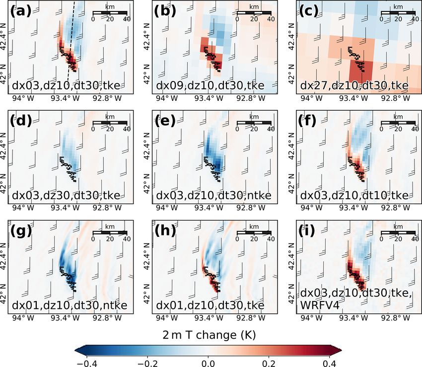
ous settings. This baseline is set to have three nested mined via comparisons of model solutions of the wind farm
domains with horizontal resolutions of 27, 9, and 3 km, re- wake, including the area of wake coverage and the magnitude
spectively, where the innermost, 3 km domain (dx03) covers of hub-height wind speed deficits and near-surface tempera-
the state of Iowa, centered over the simulated wind farm ture changes. All simulation configurations are outlined in
(Fig. 1). The vertical resolution of the baseline is nominally Table 2.
defined to be ∼ 10 m in the lowest 200 m (dz10), stretching
vertically thereafter. The model time step is 30 s on the outer
domain (dt30), reducing by a factor of 3 for each additional 3 Results
nest. Turbine-induced turbulence is parameterized via an
addition of TKE (tke), the default WFP option. We then vary 3.1 Performance of non-WFP WRF
the horizontal resolution (dx), vertical resolution (dz), time
step (dt), turbulence option (tke or ntke), and WRF model We first verify that the WRF simulations without the WFP,
version, 3.8.1 vs. 4.0 (V4), about this baseline configuration i.e., “no wind farm” (NWF) simulations, simulate accurate
to make up our sensitivity test (Table 2). ambient winds compared to the CWEX scanning lidar mea-
surements collected from outside the wind farm. Qualita-
Geosci. Model Dev., 13, 2645–2662, 2020 https://doi.org/10.5194/gmd-13-2645-2020
J. M. Tomaszewski and J. K. Lundquist: WRF WFP configuration affects wakes 2649
wind speed and direction against the scanning lidar further il-
lustrate the positive wind speed bias (Fig. 5a) and more west-
erly wind direction bias (Fig. 5b) by the simulations, with
the 27 km horizontal resolution simulation showing higher
biases than the 1 km one in both cases. The RMSE differ-
ences between the 27 and 1 km configurations are small in the
wind direction estimates (41.8◦ vs. 41.4◦ , respectively) but
differ more in the wind speed estimates, with the 27 km con-
figuration exhibiting an RMSE of 3.1 m s−1 compared to the
1 km RMSE of 2.8 m s−1 . Evaluation of other heights (150
and 200 m, not shown) reveal a similar pattern of higher bi-
ases in the 27 km domain than the 1 km, particularly in wind
speed.
Our comparisons of NWF simulations and scanning li-
Figure 1. Map representing the domains (starting at 27 km, nest- dar measurements are similar to those of Lee and Lundquist
ing down to 9, 3, and 1 km) of the horizontal resolution tests that (2017a), which also found good agreement in the occurrence
also serve as the outer domains for finer resolutions. Geography of the LLJ. Lee and Lundquist (2017a) noted slightly better
data provided by Matplotlib’s (Hunter, 2007) Basemap © 2011 by agreement in LLJ strength between simulations and the scan-
Jeffrey Whitaker. ning lidar (i.e., an absolute error on the order of 1 m s−1 ),
which may be related to the larger domain sizes of their sim-
ulations.
3.2 WRF WFP sensitivity to model settings
3.2.1 Impact on hub-height wind speed deficits
For an initial qualitative assessment of WRF WFP sensitivity
to model settings, we compare snapshots of the wake effect
at a single point in time among the various model config-
urations by subtracting the NWF simulation from the WFP
simulation. We select 02:00 UTC of 26 August (21:00 25 Au-
gust local time) to examine because of the presence of strong
southwesterly LLJ winds within and above the turbine ro-
tor layer and the easily discernible wake impacts across all
configurations tested, though many other time periods could
Figure 2. Schematic of the two vertical grids tested and where they have provided a similarly qualitative comparison.
typically intersect the turbine rotor layer (black circle): the ∼ 10 m The baseline simulation on 02:00 26 August (Fig. 6a)
grid (dz10) on the left in green and the ∼ 30 m grid (dz30) on the shows a clear hub-height wind speed deficit downwind of the
right in blue. wind farm, its impact extending over 40 km downwind with
a maximum wind speed deficit close to 1.5 m s−1 . Chang-
ing the horizontal resolution of the WRF WFP reveals a
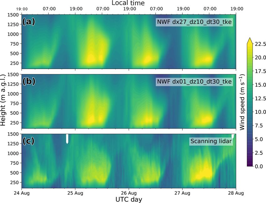
tively, all WRF configurations in our sensitivity test have clear sensitivity. Configurations with a coarser horizontal
skill in simulating the timing and position of the LLJ (a grid spacing predict wind speed deficits smaller in magni-
similar finding of Smith et al., 2019) but overestimate the tude than the baseline but spanning a larger area (Fig. 6a, b).
magnitude of the LLJ wind speed increase (Fig. 3) and pre- Conversely, a finer horizontal resolution (Fig. 6h) reduces the
dict fewer occurrences of easterly winds, especially on 24 area of impact but increases the magnitude of the wind speed
and 25 August (Fig. 4, not all configurations shown). We deficit. Coarsening the near-surface vertical resolution from
include time series of wind speed from two simulations, 10 m in the baseline simulation to 30 m impacts the model
dx27_dz10_dt30_tke (Figs. 3a, 4a) and dx01_dz10_dt30_tke solution by changing the shape of the wind speed deficit re-
(Figs. 3b, 4b), as an example. The finer horizontal resolu- gion (Fig. 6d). Disabling the WFP turbine-generated TKE
tion NWF dx01_dz10_dt30_tke better captures the intermit- option also only slightly impacts the shape of the wind speed
tency in strength of the LLJ (Fig. 3a), though both simu- deficit, although it has negligible impacts on its magnitude
lations overestimate wind speed compared to the scanning (Fig. 6e), regardless of horizontal grid spacing (Fig. 6g, h).
lidar. Comparisons of the simulated near-hub-height hourly Using WRF version 4.0 (Fig. 6i) also creates subtle differ-
https://doi.org/10.5194/gmd-13-2645-2020 Geosci. Model Dev., 13, 2645–2662, 2020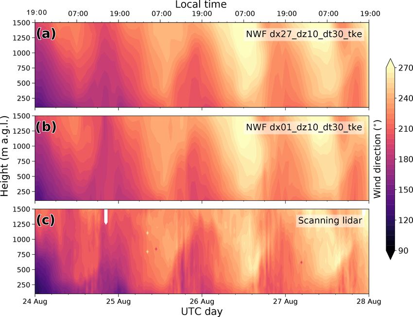
2650                                       J. M. Tomaszewski and J. K. Lundquist: WRF WFP configuration affects wakes

Figure 3. Time–height cross sections comparing wind speed from (a) the no wind farm (NWF) run of the dx27_dz10_dt30_tke simulation
with (b) the NWF run of dx01_dz10_dt30_tke, and (c) the scanning lidar observations.

Figure 4. Time–height cross sections comparing wind direction from (a) the no wind farm (NWF) run of the dx27_dz10_dt30_tke simulation
with (b) the NWF run of dx01_dz10_dt30_tke, and (c) the scanning lidar observations.

Geosci. Model Dev., 13, 2645–2662, 2020                                               https://doi.org/10.5194/gmd-13-2645-2020
J. M. Tomaszewski and J. K. Lundquist: WRF WFP configuration affects wakes 2651
Fig. 7b, predicting slightly larger regions of relatively weaker
wake impacts, following the trend of the coarser-horizontal-
resolution simulations. The newer version of WRF predicted
a similar time series of deficits as the baseline (green) but
was omitted from Fig. 7 to reduce clutter.
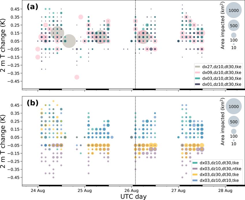
We next integrate the areas impacted by each defined
deficit value in time across the full period (Fig. 8) to corrobo-
rate earlier suggestions of sensitivity to model configuration
in Figs. 6 and 7. The coarser-horizontal-grid-spacing simu-
lations predict the largest overall region, with weaker wind
Figure 5. Hourly values of 90 m (a) wind speed (WS) and (b) wind speed deficits than the finer-grid-spacing simulations. Ad-
direction (WD) from two of the simulations tested plotted against ditionally, the coarse-vertical-resolution simulation produces
those of the scanning lidar. Dots, lines of best fit, and their corre- smaller regions of strong wake impacts (> 1.6 m s−1 deficits)
sponding equations and RMSE calculations in both panels are col- than its finer-vertical-resolution counterparts. Throughout
ored based on the model configuration denoted in the legend. One-
the range of waking magnitudes, the original baseline simu-
to-one lines are dashed in black.
lation (3 km horizontal resolution, green) closely matches the
fine-resolution (1 km) simulation’s estimates of wake cover-
age, suggesting WRF WFP estimates of wake impact and
ences in the shape of the far wake and in the magnitude of spatial coverage begin to converge at 3 km horizontal grid
the deficit in the near wake. spacing (Fig. 8). Disabling the WFP TKE term has minimal
To explicitly quantify differences between the tested con- impact between the two 1 km (red vs. dark purple) and two
figurations, we sum the total area impacted by a particular 3 km (light purple vs. green) simulation pairs examined when
magnitude of waking impact (e.g., wind speed deficit) in considering wind speed deficit effects. Differences between
hourly increments. For example, the area impacted by an the baseline’s 30 s time step and the reduced, 10 s time step
80 m wind speed deficit of 1 m s−1 in the baseline simula- simulation (blue) are small. The baseline case run with ver-
tion on 26 August at 02:00 UTC (Fig. 6a) is calculated to be sion 3.8.1 and the case run with version 4.0 (green vs. or-
about 80 km2 (denoted at the dashed black line in Fig. 7). We ange) predict similar total waking impacts over the period,
repeat the calculation for several defined deficits of interest deviating most (∼ 100 km2 ) at the 1.8 m s−1 deficit (Fig. 8).
for each hour in the period for all simulations (Fig. 7). To supplement Fig. 8, we next compare the average wake
This time series of wake impact areas gives insight on the effects predicted by the different simulation cases (Fig. 9).
temporal variability of waking, as we see the largest areas As previously noted, the coarser-horizontal-resolution sim-
of impact (larger dots in Fig. 7) and the strongest magni- ulations predict the largest average affected regions, with
tudes of deficit occur during the night, with little to no wake weaker maximum wind speed deficits than the finer-
impact areas present during the day when increased ambi- resolution simulations. Differences between average wake
ent turbulence erodes wakes, similar to the stability depen- impact predicted by the other configurations are more sub-
dence highlighted in Lundquist et al. (2018). As expected, tle, with those run at a 30 m vertical resolution or lacking the
all simulations exhibit larger areas impacted by lower deficit WFP TKE term deviating most from the baseline (green).
magnitudes (0.4–0.6 m s−1 ) relative to instances of stronger Subtle sensitivity exists to the model time step and version,
deficits (> 1 m s−1 ). Clear differences emerge in the details most apparent in the average areas impacted by the strongest
of wake area coverage between the model configurations, es- deficits, i.e., 1.8 and 2.0 m s−1 (Fig. 9). Such large deficits
pecially when horizontal resolution is varied (Fig. 7a). As occur more infrequently than others, meaning averages could
the horizontal resolution is coarsened from 1 km (dark pur- exaggerate the differences between configurations there.
ple), to 3 km (green), to 9 km (pink), and finally to 27 km
(gray), the simulation increasingly fails to capture higher- 3.2.2 Impact on near-surface temperature and
magnitude wake impacts and instead predicts larger areas of moisture changes
minor deficits.
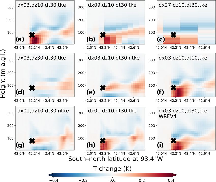
The spatial extent of wind speed deficit impact appears to Another wind farm wake effect sensitive to WRF WFP model
be most sensitive to horizontal resolution and is less sen- settings is the presence and sign of near-surface temperature
sitive to the other model settings tested (Fig. 7b). Hold- changes. As with the wind speed deficit analysis (Fig. 6),
ing horizontal resolution constant and reducing the model initial comparisons of snapshots of the temperature changes
time step (blue) or disabling the WFP turbulence generation on 26 August at 02:00 UTC reveal differences between the
(light purple) does not cause significant changes to the sim- configurations (Figs. 10, 11). The baseline simulation shows
ulations’ wind speed deficit extent across the range of im- a clear nighttime warming signal at 2 m in the immediate
pact magnitudes examined. The simulation with coarse ver- vicinity of the wind turbines (Fig. 10a), consistent with satel-
tical grid spacing (yellow) differs most from the others in lite observations (Zhou et al., 2012) and in situ observations
https://doi.org/10.5194/gmd-13-2645-2020 Geosci. Model Dev., 13, 2645–2662, 2020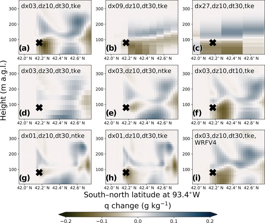
2652                                           J. M. Tomaszewski and J. K. Lundquist: WRF WFP configuration affects wakes

Figure 6. Hub-height (∼ 80 m) wind speed (WS) deficits resulting from the presence of the wind farm in the tested simulations on 26 August
02:00 UTC (25 August 21:00 LT). The 80 m wind barbs from the wind farm simulation are plotted in knots every 27 km, regardless of
horizontal resolution. The dashed line in panel (a) denotes the location of the vertical cross section in Fig. 11. Panels are cropped to the same
region around the wind farm despite certain configurations having varying simulation domains depending on horizontal resolution.

(Rajewski et al., 2013). This warming is caused by a redis-                cells at turbine hub height that does not mix down to the sur-
tribution of heat mixed down from hub height (Fig. 11a), as                face (Fig. 11d, e, g). This cooling signal produced by simula-
shown by a concurrent vertical slice transecting south–north               tions with too coarse a vertical resolution or lacking turbine-
through the wind farm (dashed line in Fig. 10a). Changing                  generated TKE directly conflicts with wind farm wake ob-
the horizontal resolution of the WRF WFP has a notable                     servations of localized near-surface warming during stable
impact on the spatial coverage of the near-surface warm-                   conditions (e.g., Zhou et al., 2012; Rajewski et al., 2013).
ing. Simulations with coarser horizontal resolutions predict               All configurations produce cooling just above turbine hub
weaker 2 m temperature warming signals that span greater                   height and warming within the rotor layer, illustrating the re-
areas (Figs. 10b, c; 11b, c), which parallel results from the              distribution of heat that occurs from mixing of the nocturnal
wind speed deficit analysis (Fig. 6b, c). Similarly, reducing              inversion; however, sufficient vertical resolution and turbine-
the time step or using WRF version 4.0 has little impact on                generated turbulence is required to mix warmer temperatures
the model solution of temperature changes based on the snap-               down to the surface (Fig. 11).
shots from Figs. 10f and i and 11f and i.                                     We sum at hourly increments the total area impacted by
   Changes to turbine-generated turbulence and vertical res-               a particular magnitude of near-surface temperature change
olution exert the greatest impacts on model solutions of tem-              to explicitly quantify differences between tested configura-
perature signals. Coarsening the vertical grid spacing from                tions (Fig. 12). We limit the bounding area of interest to grid
10 to 30 m reverses the sign of the near-surface temperature               cells immediately around the wind farm to consider the more
change, producing an unphysical localized region of surface                localized nature of near-surface temperature impacts, as op-
cooling in the immediate vicinity of the wind farm (Figs. 10d,             posed to the larger downwind fetch impacted by a wind speed
11d). Similarly, disabling turbine-generated turbulence also               deficit considered in Fig. 7. The temporal variability of wak-
causes a cooling signal near the surface, irrespective of hori-            ing again appears, with relatively larger areas of temperature
zontal resolution (Figs. 10e, g; 11e, g). Temperature profiles             impacts occurring overnight, typically emerging as a warm-
from these configurations reveal slight warming within grid                ing signal. These temperature impacts are clearly sensitive to

Geosci. Model Dev., 13, 2645–2662, 2020                                                      https://doi.org/10.5194/gmd-13-2645-2020
J. M. Tomaszewski and J. K. Lundquist: WRF WFP configuration affects wakes                                                                 2653

Figure 7. Time series of area impacted by the wake-induced, 80 m wind speed deficits as predicted by the tested simulations, plotted every 3 h
throughout the period. The size of the dots represents the spatial coverage of their respective magnitude of impact (scale denoted in top right),
with each dot colored based on its configuration. Areas of impact were calculated for deficits every 0.1 m s−1 between 0.4 and 1.0 m s−1 , then
every 0.2 until 2.0 m s−1 . The configurations are divided into groups that (a) vary horizontal resolution and (b) hold horizontal resolution
constant and vary other model settings. The time chosen for the qualitative analysis (26 August 02:00 UTC) in Fig. 6 is denoted by the black
dashed line. Black and white bar at bottom denotes post-sunrise (white) and post-sunset (black) times.

                                                                           Figure 9. Average area affected by each 80 m wind speed deficit
Figure 8. Total area impacted by the wake-induced, 80 m wind               (columns) over the entire simulation period for each simulation
speed deficits as predicted by the tested simulations, plotted at dif-     tested (rows). Yellow squares indicate larger areas of impact, with
ferent magnitudes of impact and integrated in time across the entire       empty (white) squares indicating a lack of occurrence for that par-
period. Each line is colored based on its configuration.                   ticular magnitude of impact.

                                                                           and fails to capture higher-magnitude temperature increases.
horizontal grid spacing throughout the time period (Fig. 12a).             Occasional instances of cooling occur typically just before
As the horizontal resolution is coarsened from 1 km (dark                  sunset and are exaggerated in coarser-horizontal-resolution
purple), to 3 km (green), to 9 km (pink), and finally to 27 km             configurations, likely caused by convection in the daytime
(gray), the simulation predicts larger areas of minor deficits             with locations shifted due to the presence of the wind farm.

https://doi.org/10.5194/gmd-13-2645-2020                                                       Geosci. Model Dev., 13, 2645–2662, 2020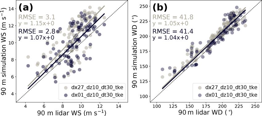
2654                                           J. M. Tomaszewski and J. K. Lundquist: WRF WFP configuration affects wakes

Figure 10. Near-surface (2 m) temperature (T ) changes resulting from the presence of the wind farm in the tested simulations on 26 August
02:00 UTC (25 August 21:00 LT). The 80 m wind barbs from the wind farm simulation are plotted in knots every 27 km, regardless of
horizontal resolution. The dashed line in panel (a) denotes the location of the vertical cross section in Fig. 11. Panels are cropped to the same
region around the wind farm despite certain configurations having varying simulation domains depending on horizontal resolution.

   Coarsening vertical resolution to 30 m (yellow) or dis-                 iterates that significant model sensitivities exist. The config-
abling TKE generation (light purple) incorrectly produces a                urations without turbine-generated turbulence at both 1 and
nocturnal cooling signal across the time period (Fig. 12b),                3 km horizontal resolutions (red, purple, respectively) or with
most notably on 25 through 27 August. WRF WFP needs to                     a coarse, 30 m, vertical resolution (yellow) exhibit the largest
be able to resolve wind shear to vertically mix warmer inver-              erroneous overall areas of significant cooling signals in the
sion air to the surface as documented in observations (e.g.,               vicinity of the wind farm (Figs. 13, 14). The 9 km horizontal
Rajewski et al., 2013; Smith et al., 2013; Rajewski et al.,                resolution (pink) also experiences relatively stronger cool-
2016; Platis et al., 2018; Siedersleben et al., 2018a), and                ing impacts across the period but estimates total areas im-
these configurations with too coarse a vertical grid spacing               pacted by warming to span hundreds of kilometers more.
(30 m) or lacking turbine-generated TKE clearly fail to gen-               Other configurations that experience cooling with adequate
erate such wind shear throughout most of the period. An ex-                (10 m) vertical grid spacing and the turbine-TKE enabled es-
ception occurs on 24 August, when more southeasterly winds                 timate such cooling to be minimal in total coverage and mag-
(Fig. 4) aligning with the orientation of the wind farm cause              nitude (Figs. 13, 14).
a narrow, highly concentrated wake region that permits the                    All configurations predict some warming immediately
30 m vertical resolution configuration to produce a surface                around the wind farm throughout the period (Figs. 13, 14),
warming signal. While WRF WFP wake effects experience                      while those with the 30 m vertical grid or lacking turbine-
strong sensitivity to vertical resolution and TKE generation,              generated TKE produce the smallest areas of warming. Con-
reducing the model time step (blue) from the baseline (green)              figurations with the coarsest horizontal resolutions (27 km,
has little impact on the temperature change solution through-              gray; 9 km, pink) predict large areas of impact by weak
out the period (Fig. 12b).                                                 warming signals. Only configurations with a 3 km or finer
   As with the wind speed deficit analysis, we next integrate              horizontal grid are able to capture warming impacts above
(Fig. 13) and average (Fig. 14) the areas impacted by each                 0.4 K. Reducing model time step (blue) or using version 4.0
defined deficit value in time across the full period, which re-            of WRF (orange) again has little impact on the overall predic-

Geosci. Model Dev., 13, 2645–2662, 2020                                                      https://doi.org/10.5194/gmd-13-2645-2020
J. M. Tomaszewski and J. K. Lundquist: WRF WFP configuration affects wakes                                                        2655

Figure 11. Vertical cross sections of temperature (T ) changes resulting from the presence of the wind farm in the tested simulations on
26 August 02:00 UTC (25 August 21:00 LT). The median location and hub height of the wind farm is denoted by the black X. Location of
this slice is denoted by the dashed line in Fig. 10.

tion of temperature impact coverage compared to the base-             simulations with too coarse a vertical resolution or lacking
line (green) (Figs. 13, 14).                                          turbine-generated TKE contradicts observations of localized
   Another impact of wind farm wakes is the changes to the            near-surface drying during stable conditions (Baidya Roy,
near-surface moisture content, which can happen overnight             2004; Siedersleben et al., 2018a), implying that those sim-
when the enhanced mixing from the wind farm brings rel-               ulations lack sufficient mixing, the same deficiency that pro-
atively drier air down and moister air up, leading to a dry-          duces erroneous cooling signals (Fig. 11) as well. We omit
ing near the surface and moistening aloft (Baidya Roy, 2004;          discussing the model sensitivity in producing moisture im-
Siedersleben et al., 2018a). We examine the model sensi-              pacts with the same detail as the temperature changes, as the
tivity in producing this moisture effect via a vertical snap-         moisture impact results parallel those of the temperature im-
shot of water vapor mixing ratio (q) changes on 26 August             pacts.
at 02:00 UTC (Fig. 15). As with the temperature analysis
(Fig. 11), changing the horizontal resolution of the WRF
WFP has a notable impact on the spatial coverage and inten-
sity of the near-surface drying. Simulations with coarser hori-       4   Discussion
zontal resolutions predict weaker near-surface drying signals
that span larger areas (Fig. 15b, c).                                 We compare different WRF WFP simulation solutions of
   However, changes to turbine-generated turbulence and               land-based wind farm wake effects in simple terrain and me-
vertical resolution have the greatest impacts on model solu-          teorological conditions to quantify the sensitivity of the sim-
tions of moisture signals. Coarsening the vertical grid spac-         ulations to model configuration and thereby define recom-
ing from 10 to 30 m reverses the sign of the moisture change,         mendations for best-practice model settings. Settings tested
producing a localized region of surface moistening in the im-         include horizontal and vertical grid spacing, model time step,
mediate vicinity of the wind farm (Fig. 15d). Similarly, dis-         model version, and inclusion of turbine-generated turbu-
abling turbine-generated turbulence also causes an increase           lence. We divide our analysis into the two main atmospheric
in water vapor near the surface, irrespective of horizontal           impacts of a wind farm wake: a hub-height wind speed deficit
resolution (Fig. 15e, g). This moistening signal produced by          extending downwind of the wind farm and a nighttime near-

https://doi.org/10.5194/gmd-13-2645-2020                                                 Geosci. Model Dev., 13, 2645–2662, 2020
2656                                         J. M. Tomaszewski and J. K. Lundquist: WRF WFP configuration affects wakes

Figure 12. Time series of area impacted by the wake-induced, 2 m temperature changes as predicted by the tested simulations, plotted every
2 h throughout the period. The size of the dots represents the spatial coverage of their respective magnitude of impact (scale denoted in
top right), with each dot colored based on its configuration. The configurations are divided into groups that (a) vary horizontal resolution
and (b) hold horizontal resolution constant while varying other model settings. The time chosen for the qualitative analysis (26 August
02:00 UTC) in Fig. 6 is denoted by the black dashed line. Black and white bar at bottom denotes post-sunrise (white) and post-sunset (black)
times.

                                                                        Figure 14. Average area affected by each 2 m temperature change
Figure 13. Total area impacted by the wake-induced 2 m temper-          (columns) over the entire simulation period for each simulation
ature change as predicted by the tested simulations, plotted at dif-    tested (rows). Yellow squares indicate larger areas of impact, with
ferent magnitudes of impact and integrated in time across the entire    empty (white) squares indicating a lack of occurrence for that par-
period. Each line is colored based on its configuration. Areas of       ticular magnitude of impact.
warming are summed separately from areas of cooling.

                                                                        izontal grids of 3 and 1 km converged on similar depictions
surface temperature increase immediately around the wind                of the magnitude and spatial coverage of wind deficits, while
farm mixed down from the nocturnal inversion.                           grids of 9 km or larger dilute the wake impact over large ar-
   In summary, simulated WRF WFP solutions of wind speed                eas. Solutions of 2 m temperature (and similarly moisture)
deficits are most sensitive to the horizontal resolution. Hor-          changes are also sensitive to horizontal resolution in that too

Geosci. Model Dev., 13, 2645–2662, 2020                                                   https://doi.org/10.5194/gmd-13-2645-2020
J. M. Tomaszewski and J. K. Lundquist: WRF WFP configuration affects wakes 2657 Figure 15. Vertical cross sections of water vapor mixing ratio (q) changes resulting from the presence of the wind farm in the tested simulations on 26 August 02:00 UTC (25 August 21:00 LT). The median location and hub height of the wind farm is denoted by the black X. Location of this slice is denoted by the dashed line in Fig. 10. coarse (> 9 km) a grid spacing results in large expanses of innermost turbine-containing domain are thus recommended. weak temperature changes, contradicting the typically local- Close similarities between the 1 and 3 km configurations sug- ized nature of temperature impacts from a wind farm seen in gest the user can confidently produce accurate waking with observations (e.g., Baidya Roy, 2004; Zhou et al., 2012; Ra- a 3 km WRF WFP grid spacing, refining to 1 km if the com- jewski et al., 2013; Siedersleben et al., 2018a). The more im- putation resources are available or if terrain complexity indi- portant model settings to consider for accurate representation cates that finer resolution is required. of surface temperature impacts of wind farm wakes, however, The choice of vertical resolution significantly impacts are the vertical resolution and turbine-generated turbulence WRF WFP solutions of wake effects, especially in the repre- term, as a too coarse (i.e., 30 m) vertical grid or a lack of sentation of nocturnal near-surface warming around the wind additional turbine turbulence fails to simulate enough wind farm (Figs. 10d, 11d, 12b, 13, 14). A 30 m vertical grid con- shear to vertically mix warm inversion air to the surface, re- sistently produces more incorrect cooling signals overnight sulting in an incorrect surface cooling signal overnight. than the baseline simulation with a 10 m grid. Observed sur- Out of the four horizontal resolutions tested, the finer-grid face warming in the vicinity of wind farms occurs because of (1 and 3 km) configurations produce a more robust repre- the turbine-generated turbulence mixing down warm air from sentation of wind farm wakes than the coarser grids (9 and above the nighttime inversion to the surface (Baidya Roy, 27 km). The finer grid spacing allows stronger wake impacts 2004; Baidya Roy and Traiteur, 2010; Zhou et al., 2012; both in the wind speed deficit and surface warming to de- Rajewski et al., 2013). A sufficiently refined vertical grid is velop over a more localized region, better matching obser- thus necessary to resolve this downward mixing, and a 30 m vations (e.g., Siedersleben et al., 2018a). Coarser horizontal grid is inadequate. These findings support prior work in Lee grids (> 9 km) have been chosen in recent work (e.g., Vau- and Lundquist (2017a), which also concluded that a finer tard et al., 2014; Miller and Keith, 2018) for long-term or (∼ 12 m) vertical grid is favorable for the separate purpose of spatially large simulations because of the savings in compu- producing more accurate WRF WFP solutions of the winds tational expenses (see Table 2). However, such simulations and power production than a coarser (∼ 22 m) grid. However, imply a broader region of impact than is realistic (Figs. 6, 7, coarse (> 20 m) vertical resolutions have been employed in 8, 9). Configurations on the order of a few kilometers in the other past WRF WFP studies, possibly artificially constrain- https://doi.org/10.5194/gmd-13-2645-2020 Geosci. Model Dev., 13, 2645–2662, 2020
2658                                      J. M. Tomaszewski and J. K. Lundquist: WRF WFP configuration affects wakes

ing the temperature signal (e.g., occurrence of both negative     turbulence option in the WFP has little impact on the wind
and positive temperature signals seen in Vautard et al., 2014).   speed deficit solution, disabling it results in an inaccurate
   In addition, the turbine-induced turbulence option has sim-    cooling signal beneath the wind farm. Similarly, a coarse
ilar impacts on the WRF WFP wake solution as the verti-           (30 m) vertical resolution has minimal impact on the rep-
cal resolution. When enabled, this turbulence option within       resentation of the wind deficit aloft but impacts the surface
the WFP adds an additional source of TKE within turbine-          temperature signal drastically by reversing the sign of the ex-
containing grid cells derived from the difference between         pected temperature impact. WRF WFP simulations thus re-
the turbine thrust and power coefficients. Without this added     quire a ∼ 10 m low-level vertical grid as well as the turbine-
TKE source, WRF wind farm wake turbulence only devel-             turbulence option enabled to produce the wind shear neces-
ops because of the wind shear that arises out of the mo-          sary to vertically mix the inversion air and attain the expected
mentum deficit aloft in the wind farm wake. However, this         surface warming and drying. Horizontal resolution affects
shear-induced mixing is insufficient, as configurations with-     both the wind speed deficit and surface warming: a too coarse
out the added turbine-TKE option consistently produce inac-       (> 9 km) grid dilutes wake effect intensity over greater areas,
curate nocturnal cooling signals at the surface immediately       while grids of 1 km or 3 km converge on similar depictions
beneath the wind farm (Figs. 10e, g, 11e, g, 12b, 13, 14).        of the magnitude and spatial coverage of wake impacts and
Such surface cooling implies that insufficient mixing is oc-      thus serve as our recommended horizontal grid choice.
curring within WRF WFP, making it unable to bring warm               In conclusion, the WRF WFP is sensitive to certain model
inversion air to the surface. This hypothesis is corroborated     settings, particularly (1) the horizontal resolution in produc-
by Xia et al. (2019), which demonstrated that the WFP tur-        ing accurate intensity and coverage of the wind speed deficit
bulence option is responsible for the surface warming sig-        and surface temperature change and (2) the vertical resolu-
nal through the enhancement of vertical mixing. As such, the      tion and (3) turbine turbulence option in producing the cor-
WFP turbine TKE option, in addition to sufficiently refined       rect surface warming signal. In order to obtain the most ac-
vertical and horizontal grid resolutions (∼ 10 m and ∼ 3 km,      curate representation of wind farm wakes, we suggest that
respectively), is required to represent wind farm wakes accu-     users define a horizontal grid for the turbine-containing do-
rately.                                                           main on the order of a few kilometers and a vertical grid
                                                                  near 10 m in the lowest ∼ 200 m. The inclusion of turbine-
                                                                  generated turbulence is also necessary. While model time
5   Conclusions                                                   step and model version had less impact on the wake solu-
                                                                  tions, these sensitivity evaluations should continue as WRF
As wind energy continues to rapidly develop, the Wind Farm        and the PBL schemes evolve.
Parameterization (WFP) within the Weather Research and               This sensitivity study and subsequent model setting rec-
Forecasting (WRF) model provides a means for simulating           ommendations are derived from analysis of a single location
wind farms and their large-scale wake effects. However, lit-      and time period, and further analysis including a wider range
tle guidance currently exists for choice in model settings to     of meteorological conditions or locations could be worth-
produce the most accurate solution of wakes. Herein, we as-       while, especially as wind energy develops more offshore
sess the sensitivity of the WRF WFP to model configuration        and in complex terrain on land. While we predict the WFP
to provide recommended settings for simulating wind farm          wake solutions and model sensitivity in less-turbulent off-
wakes effects.                                                    shore environments will behave similarly to the simple ter-
   We select 24–27 August of the 2013 Crop Wind Experi-           rain case studied herein, the more turbulent flow over com-
ment (CWEX-13) field campaign as our case study because           plex topography may alter how wakes are represented in the
of the simple terrain, availability of observations, and con-     WRF WFP and thus impact the model sensitivity. The WFP
sistent, nocturnal low-level jet occurrences without interfer-    is designed to work with the MYNN 2.5 level PBL scheme,
ence from large-scale synoptic meteorological events. We          so impacts that the choice in PBL scheme may have on
use measurements from a scanning lidar to first verify the        the background meteorology and subsequent wake solution
ambient flow simulated by WRF before implementing the             are not addressed. Furthermore, within-the-grid-cell turbine
WFP and varying the horizontal and vertical resolutions,          wake interactions are omitted in the WFP and not consid-
turbine-generated turbulence, model version, and model time       ered here. Future applications of the WRF WFP to investi-
step settings to comprise the sensitivity analysis. Each model    gate wind farm wake effects will have scientific and societal
configuration simulates a real Iowa wind farm containing 200      implications, so it is therefore important to consider model
1.5 MW turbines.                                                  settings when designing simulations.
   We isolate the impacts of WRF WFP settings on the two
predominant meteorological effects of a wind farm wake, the
hub-height wind speed deficit and the transient surface tem-      Code and data availability. The  WRF-ARW     model     code
perature increase arising out of downward mixing of the noc-      (https://doi.org/10.5065/D6MK6B4K, Skamarock et al., 2008)
turnal inversion. While the inclusion of the turbine-generated    is publicly available at http://www2.mmm.ucar.edu/wrf/users/

Geosci. Model Dev., 13, 2645–2662, 2020                                           https://doi.org/10.5194/gmd-13-2645-2020
J. M. Tomaszewski and J. K. Lundquist: WRF WFP configuration affects wakes 2659
(last access: 11 June 2020). This work uses the WRF-ARW ing large-eddy simulation, Geophys. Res. Lett., 40, 4963–4970,
model and the WRF Preprocessing System (WPS) version 3.8.1 https://doi.org/10.1002/grl.50911, 2013.
(released on 12 August 2016), and the wind farm parameter- Astolfi, D., Castellani, F., and Terzi, L.: A Study of Wind Tur-
ization is distributed therein. Initial and boundary conditions bine Wakes in Complex Terrain Through RANS Simulation
are provided by Era-Interim (Dee et al., 2011) available at and SCADA Data, J. Sol. Energ.-T. ASME, 140, 031001,
https://rda.ucar.edu/datasets/ds627.0/ (last access: 11 June 2020). https://doi.org/10.1115/1.4039093, 2018.
Topographic data are provided at a 30 s resolution from http: Baidya Roy, S.: Can large wind farms affect lo-
//www2.mmm.ucar.edu/wrf/users/download/get_source.html (Ska- cal meteorology?, J. Geophys. Res., 109, D19101,
marock et al., 2008). The PSU generic 1.5 MW turbine (Schmitz, https://doi.org/10.1029/2004JD004763, 2004.
2012) is available at https://doi.org/10.13140/RG.2.2.22492.18567. Baidya Roy, S. and Traiteur, J. J.: Impacts of wind farms on surface
The model namelists, wind turbine specifications, and parsed air temperatures, P. Natl. Acad. Sci. USA, 107, 17899–17904,
output data needed to recreate the figures and analysis are located https://doi.org/10.1073/pnas.1000493107, 2010.
at https://doi.org/10.5281/zenodo.3755282 (Tomaszewski, 2019). Barrie, D. B. and Kirk-Davidoff, D. B.: Weather response to a
large wind turbine array, Atmos. Chem. Phys., 10, 769–775,
https://doi.org/10.5194/acp-10-769-2010, 2010.
Author contributions. JKL and JMT conceived the research and de- Beaucage, P., Brower, M., Robinson, N., and Alonge, C.: Overview
signed the WRF simulations; JMT carried out the WRF simulations of six commercial and research wake models for large offshore
and wrote the paper with significant input from JKL. wind farms, Proceedings of the European Wind Energy Associa-
tion Conference, Copenhagen, 95 pp., 2012.
Bodini, N., Zardi, D., and Lundquist, J. K.: Three-
Competing interests. The authors declare that they have no conflict dimensional structure of wind turbine wakes as measured
of interest. by scanning lidar, Atmos. Meas. Tech., 10, 2881–2896,
https://doi.org/10.5194/amt-10-2881-2017, 2017.
Boersma, S., Gebraad, P., Vali, M., Doekemeijer, B., and
van Wingerden, J.: A control-oriented dynamic wind farm
Acknowledgements. This work and Jessica M. Tomaszewski were
flow model: “WFSim”, J. Phys. Conf. Ser., 753, 032005,
supported by an NSF Graduate Research Fellowship under grant
https://doi.org/10.1088/1742-6596/753/3/032005, 2016.
number 1144083. WRF simulations were conducted using the Ex-
Cabezón, D., Migoya, E., and Crespo, A.: Comparison of turbulence
treme Science and Engineering Discovery Environment (XSEDE),
models for the computational fluid dynamics simulation of wind
which is supported by National Science Foundation grant number
turbine wakes in the atmospheric boundary layer, Wind Energy,
ACI1053575. Julie K. Lundquist’s effort was supported by an agree-
14, 909–921, https://doi.org/10.1002/we.516, 2011.
ment with NREL under APUP UGA-0-41026-65.
Calaf, M., Meneveau, C., and Meyers, J.: Large eddy simula-
tion study of fully developed wind-turbine array boundary lay-
ers, Phys. Fluids, 22, 015110, https://doi.org/10.1063/1.3291077,
Financial support. This research has been supported by the Na- 2010.
tional Science Foundation CAREER Award (grant no. AGS- Ching, J., Rotunno, R., LeMone, M., Martilli, A., Kosoviĉ, B.,
1554055) and NSF Graduate Research Fellowship under grant num- Jimenez, P. A., and Dudhia, J.: Convectively Induced Sec-
ber 1144083. ondary Circulations in Fine-Grid Mesoscale Numerical Weather
Prediction Models, Mon. Weather Rev., 142, 3284–3302,
https://doi.org/10.1175/MWR-D-13-00318.1, 2014.
Review statement. This paper was edited by Christoph Knote and Christiansen, M. B. and Hasager, C. B.: Wake ef-
reviewed by Christoph Knote and one anonymous referee. fects of large offshore wind farms identified from
satellite SAR, Remote Sens. Environ., 98, 251–268,
https://doi.org/10.1016/j.rse.2005.07.009, 2005.
Churchfield, M. J., Lee, S., Michalakes, J., and Moriarty, P. J.:
References A numerical study of the effects of atmospheric and wake
turbulence on wind turbine dynamics, J. Turbul., 13, N14,
Abkar, M. and Porté-Agel, F.: Influence of atmospheric stability on https://doi.org/10.1080/14685248.2012.668191, 2012.
wind-turbine wakes: A large-eddy simulation study, Phys. Fluids, Dee, D. P., Uppala, S. M., Simmons, A. J., Berrisford, P., Poli,
27, 035104, https://doi.org/10.1063/1.4913695, 2015a. P., Kobayashi, S., Andrae, U., Balmaseda, M. A., Balsamo, G.,
Abkar, M. and Porté-Agel, F.: A new wind-farm parameterization Bauer, P., Bechtold, P., Beljaars, A. C. M., van de Berg, L., Bid-
for large-scale atmospheric models, J. Renew. Sustain. Ener., 7, lot, J., Bormann, N., Delsol, C., Dragani, R., Fuentes, M., Geer,
013121, https://doi.org/10.1063/1.4907600, 2015b. A. J., Haimberger, L., Healy, S. B., Hersbach, H., Hólm, E. V.,
Aitken, M. L., Kosović, B., Mirocha, J. D., and Lundquist, Isaksen, L., Kållberg, P., Köhler, M., Matricardi, M., McNally,
J. K.: Large eddy simulation of wind turbine wake dynam- A. P., Monge-Sanz, B. M., Morcrette, J.-J., Park, B.-K., Peubey,
ics in the stable boundary layer using the Weather Research C., de Rosnay, P., Tavolato, C., Thépaut, J.-N., and Vitart, F.: The
and Forecasting Model, J. Renew. Sustain. Ener., 6, 033137, ERA-Interim reanalysis: configuration and performance of the
https://doi.org/10.1063/1.4885111, 2014. data assimilation system, Q. J. Roy. Meteor. Soc., 137, 553–597,
Archer, C. L., Mirzaeisefat, S., and Lee, S.: Quantifying the sen- https://doi.org/10.1002/qj.828, 2011.
sitivity of wind farm performance to array layout options us-
https://doi.org/10.5194/gmd-13-2645-2020 Geosci. Model Dev., 13, 2645–2662, 2020You can also read