Deep Identification of Arabic Dialects - Interactive Systems ...
←
→
Page content transcription
If your browser does not render page correctly, please read the page content below
Deep Identification of Arabic Dialects

                        Bachelor’s Thesis
                               by

                         Alaa Mousa

                  Department of Informatics
         Institute for Anthropomatics and Robotics
                   Interactive Systems Labs

     First Reviewer:         Prof. Dr. Alexander Waibel
     Second Reviewer:        Prof. Dr.-Ing. Tamim Asfour
     Advisor:                Juan Hussain, M.Sc.

       Project Period:       10/11/2020 – 10/03/2021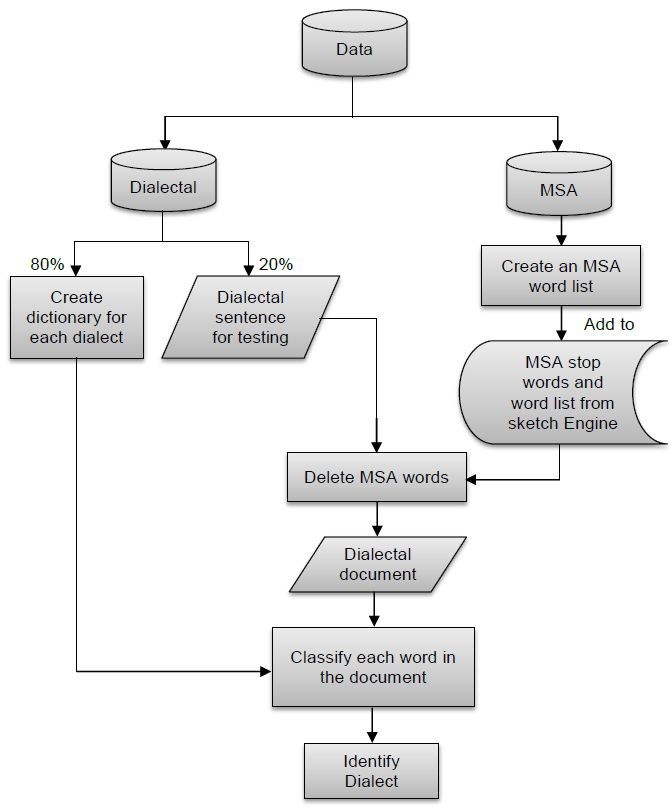
I declare that I have developed and written the enclosed thesis completely by myself,
and have not used sources or means without declaration in the text.
Karlsruhe, 01.03.2021

.....................................
           Alaa Mousa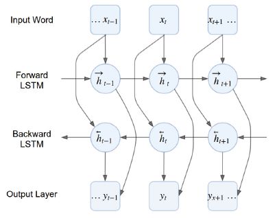
Abstract

Due to the social media revolution in the last decade, Arabic dialects have begun
to appear in written form. The problem of automatically determining the dialect of
an Arabic text remains a major challenge for researchers. This thesis investigates
many deep learning techniques for the problem of automatically identifying the
dialect of a text written in Arabic. We investigate three basic models, namely a
recurring neural network (RNN) -based model and an unidirectional, short-term
memory (LSTM) -based model, and a bidirectional LSTM-based model combined
with a self-attention network. We also explore how applying some techniques like
convolution and Word2Vec embedding on the input text can improve the achieved
accuracy. Finally, we perform a detailed error analysis that considers some individual
errors in order to show the difficulties and challenges involved in processing Arabic
texts.
Contents

1 Introduction                                                                                                1

2 Language Background                                                                                         3
  2.1 Arabic Language & Arabic Dialects . . . . . . . . . . . . . . . . . . .                                 3

3 Problem of Arabic Dialects Identification                                                                   5
  3.1 Definition . . . . . . . . . . . . . . . . . . . . . . . . . . . . . . . . .                            5
  3.2 The Difficulties & Challenges . . . . . . . . . . . . . . . . . . . . . .                                5
  3.3 Application of ADI . . . . . . . . . . . . . . . . . . . . . . . . . . . .                              6

4 Arabic Dialect Identification Approaches                                                                     7
  4.1 Minimally Supervised Approach . . . . . . . . .         .   .   .   .   .   .   .   .   .   .   .   .    7
      4.1.1 Dialectal Terms Method . . . . . . . . .          .   .   .   .   .   .   .   .   .   .   .   .    7
      4.1.2 Voting Methods . . . . . . . . . . . . . .        .   .   .   .   .   .   .   .   .   .   .   .    7
             4.1.2.1 Simple Voting Method . . . . .           .   .   .   .   .   .   .   .   .   .   .   .    8
             4.1.2.2 Weighted Voting Method . . .             .   .   .   .   .   .   .   .   .   .   .   .    8
      4.1.3 Frequent Terms Methods . . . . . . . .            .   .   .   .   .   .   .   .   .   .   .   .    9
  4.2 Feature Engineering Supervised Approach . . .           .   .   .   .   .   .   .   .   .   .   .   .    9
      4.2.1 Features Extraction . . . . . . . . . . .         .   .   .   .   .   .   .   .   .   .   .   .    9
             4.2.1.1 Bag-of-words model (BOW) . .             .   .   .   .   .   .   .   .   .   .   .   .    9
             4.2.1.2 n-gram language model . . . .            .   .   .   .   .   .   .   .   .   .   .   .    9
      4.2.2 Classification Methods . . . . . . . . . .        .   .   .   .   .   .   .   .   .   .   .   .   10
             4.2.2.1 Logistic Regression(LR) . . . .          .   .   .   .   .   .   .   .   .   .   .   .   10
             4.2.2.2 Support Vector Machine(SVM)              .   .   .   .   .   .   .   .   .   .   .   .   11
             4.2.2.3 Naive Bayes(NB) . . . . . . . .          .   .   .   .   .   .   .   .   .   .   .   .   11
  4.3 Deep Supervised Approach . . . . . . . . . . . .        .   .   .   .   .   .   .   .   .   .   .   .   12
  4.4 Related Work . . . . . . . . . . . . . . . . . . .      .   .   .   .   .   .   .   .   .   .   .   .   12

5 Deep Neural Networks                                                                                        17
  5.1 Basics of DNN . . . . . . . . . . . . . . . . .     .   .   .   .   .   .   .   .   .   .   .   .   .   17
      5.1.1 The Artificial Neuron . . . . . . . . .       .   .   .   .   .   .   .   .   .   .   .   .   .   17
      5.1.2   General Architecture of DNN . . . .         .   .   .   .   .   .   .   .   .   .   .   .   .   18
  5.2 Types of DNN . . . . . . . . . . . . . . . . .      .   .   .   .   .   .   .   .   .   .   .   .   .   19
      5.2.1 Convolutional Neural Networks(CNN)            .   .   .   .   .   .   .   .   .   .   .   .   .   19
      5.2.2 Recurrent Neural Networks(RNN) . .            .   .   .   .   .   .   .   .   .   .   .   .   .   20
  5.3 Word Embedding Techniques . . . . . . . . .         .   .   .   .   .   .   .   .   .   .   .   .   .   22
      5.3.1 skip-gram . . . . . . . . . . . . . . . .     .   .   .   .   .   .   .   .   .   .   .   .   .   22
      5.3.2 continuous bag of words (CBOW) . . .          .   .   .   .   .   .   .   .   .   .   .   .   .   22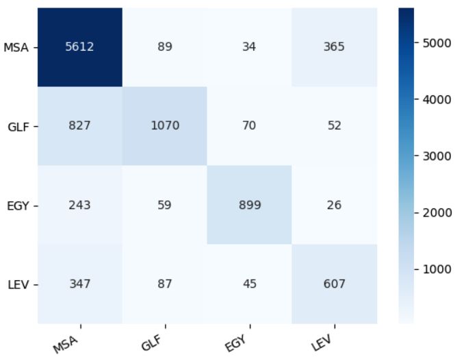
ii                                                                                     Contents

6 Methodology                                                                                      23
  6.1 Word-based recurrent neural Network (RNN): . . . . . . . . . . .                     .   .   23
  6.2 Word-based Long-Short Term Memory (LSTM): . . . . . . . . . .                        .   .   24
  6.3 Bidirectional LSTM with self attention mechanism (biLSTM-SA):                        .   .   24
  6.4 Hybrid model (CNN-biLSTM-SA): . . . . . . . . . . . . . . . . .                      .   .   25
  6.5 Hybrid model (Word2Vec-biLSTM-SA): . . . . . . . . . . . . . .                       .   .   26
  6.6 Data prepossessing . . . . . . . . . . . . . . . . . . . . . . . . . .               .   .   26

7 Evaluation                                                                                       29
  7.1 Data set . . . . . . . . . . . . . . . . . . . . . . . . . . .   .   .   .   .   .   .   .   29
  7.2 Experiments and Results . . . . . . . . . . . . . . . . . .      .   .   .   .   .   .   .   30
  7.3 Error Analysis . . . . . . . . . . . . . . . . . . . . . . . .   .   .   .   .   .   .   .   35
      7.3.1 3-Way Experiment . . . . . . . . . . . . . . . . .         .   .   .   .   .   .   .   35
      7.3.2 2-Way Experiment . . . . . . . . . . . . . . . . .         .   .   .   .   .   .   .   38
      7.3.3 4-Way Experiment . . . . . . . . . . . . . . . . .         .   .   .   .   .   .   .   39
      7.3.4 Overall Analysis and Discussion . . . . . . . . . .        .   .   .   .   .   .   .   40
             7.3.4.1 Effect of convolutional layers . . . . . .        .   .   .   .   .   .   .   41
             7.3.4.2 Effect of Word2Vec CBOW embedding                 .   .   .   .   .   .   .   41
             7.3.4.3 Effect of SentncePiece Tokenizer . . . .          .   .   .   .   .   .   .   41

8 Conclusion                                                                                       43

Bibliography                                                                                       45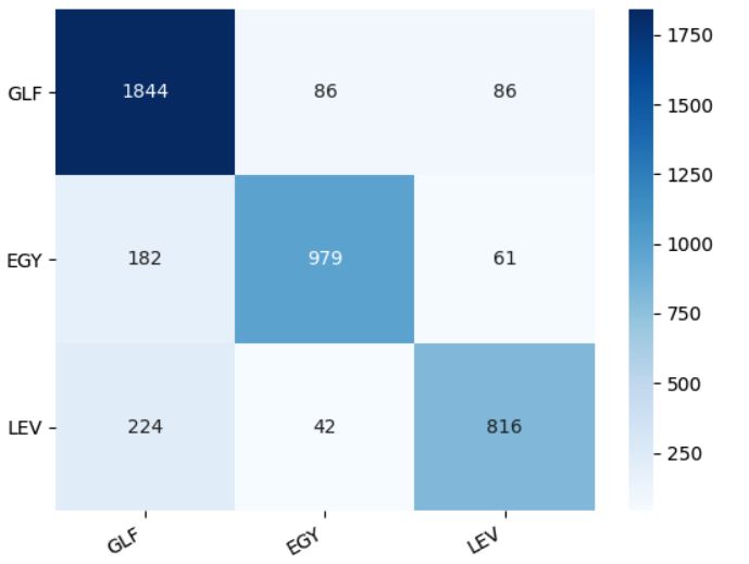
List of Figures

 2.1   Categorization of Arabic dialects in 5 main classes [58] . . . . . . . .      4

 4.1   Classification process using lexicon based approach [2]     . . . . . . . .   8
 4.2   SVM classifier identifies the hyperplane in such a way that the dis-
       tance between the two classes is maximal [8] . . . . . . . . . . . . . 11
 4.3   Classify the new white data point with NB classifier [53] . . . . . . . 12

 5.1   The artificial neuron [46] . . . . . . . . . . . . . . . . . . . . . . . . . 17
 5.2   Sigmoid function [46] . . . . . . . . . . . . . . . . . . . . . . . . . . . 18
 5.3   Hyperbolic tangent function [46] . . . . . . . . . . . . . . . . . . . . . 18
 5.4   Multi-Layer Neural Network [56] . . . . . . . . . . . . . . . . . . . . 19
 5.5   Typical Convolutional Neural Network [55] . . . . . . . . . . . . . . . 20
 5.6   Recurrent Neural Network [46]      . . . . . . . . . . . . . . . . . . . . . 20
 5.7   Long Short-term Memory Cell [19] . . . . . . . . . . . . . . . . . . . 21
 5.8   Bidirectional LSTM Architecture [46] . . . . . . . . . . . . . . . . . . 21
 5.9   The architecture of CBOW and Skip-gram models [36] . . . . . . . . 22

 6.1   biLSTM with self-attention mechanism [31] . . . . . . . . . . . . . . 24
 6.2   CNN-biLSTM-SA model          . . . . . . . . . . . . . . . . . . . . . . . . 26
 6.3   Word2Vec-biLSTM-SA model . . . . . . . . . . . . . . . . . . . . . . 26

 7.1   Heat map illustrates the percentage of shared vocabularies between
       varieties in dataset [11]. Please note that this matrix is not symmetric
       and can be read for example as follows: The percentage of EGY words
       in GLF is 0.08, whereas the percentage of GLF words in EGY is 0.06. 30
 7.2   The confusion matrix for 2-way-experiment where the classes on the
       left represent the true dialects and those on the bottom represent the
       predicted dialects by drop-biLSTM-SA model . . . . . . . . . . . . . 33
 7.3   The confusion matrix for 3-way-experiment where the classes on the
       left represent the true dialects and those on the bottom represent the
       predicted dialects by drop-biLSTM-SA model . . . . . . . . . . . . . 34
iv List of Figures
7.4 The confusion matrix for 4-way-experiment where the classes on the
left represent the true dialects and those on the bottom represent the
predicted dialects by drop-biLSTM-SA model . . . . . . . . . . . . . 34
7.5 The probabilities for classifying the sentence in the first example . . 35
7.6 The probabilities for classifying the sentence in the second example . 37List of Tables
4.1 summarizing of related works, where in feature column W denote to
word and Ch denote to character. The varieties MSA, GLF , LEV,
EGY, DIAL represented with M, G, L ,E ,D, respectively and North
African dialect with N, for simplicity. . . . . . . . . . . . . . . . . . . 15
7.1 The number of sentences for each Arabic variety in dataset [11] . . . 29
7.2 Shared Hyper parameters over all experiments . . . . . . . . . . . . . 31
7.3 Achieved classification accuracy for 2-way-Experiment . . . . . . . . 31
7.4 Achieved classification accuracy for 3-way-Experiment . . . . . . . . 31
7.5 Achieved classification accuracy for 4-way-Experiment . . . . . . . . 32
7.6 Achieved classification accuracy with drop-biLSTM-SA for all exper-
iments . . . . . . . . . . . . . . . . . . . . . . . . . . . . . . . . . . . 32
7.7 Achieved classification accuracy with Bpe-drop-biLSTM-SA for 3-
way-experiment . . . . . . . . . . . . . . . . . . . . . . . . . . . . . . 32
7.8 Hyper parameter values with which we got the best results for the
model drop-biLSTM-SA . . . . . . . . . . . . . . . . . . . . . . . . . 33
7.9 The most repeated words for EGY in our training data set . . . . . . 36
7.10 The most repeated words for LEV in our training data set . . . . . . 36
7.11 The most repeated words for GLF in our training data set . . . . . . 38
7.12 The most repeated words for DIAL in our training data set . . . . . . 39vi List of Tables
Chapter 1

Introduction

The process of computationally identifying the language of a given text is considered
the cornerstone of many important NLP applications such as machine translation,
social media analysis, etc. Since the dialects could be considered as a closely related
languages, dialect identification could be referred to as a special (more difficult)
case of language identification problem. Previously, written Arabic was mainly
using a standard form known as Modern Standard Arabic (MSA). MSA is the official
language in all countries of Arabic world; it is mainly used in formal and educational
contexts, such as news broadcasts, political discourse, and academic events. In the
last decade, Arabic dialects have begun to be represented in written forms, not
just spoken ones. The emergence of social media and the World Wide Web has
played a significant role in this development in the first place due to their interactive
interfaces. As a result, the amount of written dialectal Arabic (DA) has increased
dramatically. This development has also generated the need for further research,
especially in fields like Arabic Dialect Identification (ADI).
The language identification problem has been classified as solved by McNamee in
[34]; unfortunately, this is not valid in the case of ADI, due to the high level of
morphological, syntactic, lexical, and phonological similarities among these dialects
(Habash [23]). Since these dialects are used mainly in unofficial communication
on the world wide web, comments on online newsletters, etc., they generally tend
to be corrupt, and of lower quality (Diab [10]). Furthermore, in writing online
content (comments, blogs, etc.) writers often switch between MSA and one or more
other Arabic dialects. All of these factors contribute to the fact that the mission
of processing Arabic dialects presents a much greater challenge than working with
MSA. Accordingly, we have seen a growing interest from researchers in applying
NLP research to these dialects over the past few years.
In this thesis, we perform some classification experiments on Arabic text data con-
tains 4 Arabic varieties: MSA, GLF, LEV and EGY. The goal of these experiments
is to automatically identify the variety of each sentence in this data using the best
deep neural network techniques proposed in the literature and which proved the best
results. For our experiments we use three baseline models which are a word based
recurrent neural network RNN, a word based unidirectional long-short term mem-
ory LSTM and a bidirectional LSTM with self attention mechanism (biLSTM-SA)
introduced in (Lin et al. [31]) which proved its effectiveness for sentiment analysis
problem. In order to improve the results and gain more accuracy in our experiments
2                                                                    1. Introduction

we add more components for the biLSTM-SA model, which achieved the best re-
sults. First, we add two convolutional layers to this model in order to gain more
semantics features, especially between the neighboring words in the input sequence,
before they passed on to LSTM layer. Where we were inspired with this idea from
the work of (Jang et al.[25]). Second, we perform a continuous bag of words CBOW
embedding over the training data set to gain a thoughtful word encoding that in-
cludes some linguistic information as initialization, instead of random embedding,
hoping to improve the classification process. We also test two types of tokeniza-
tion for our best model, namely, the white space tokenization and sentence piece
tokenization.
We use for our experiments the Arabic Online Commentary dataset (AOC) intro-
duced by (Zaidan et al.[57]) which contains 4 Arabic varieties, namely, MSA. EGY,
GLF and LEV. We perform three main experiments: The first one is to classify
between MSA and dialectal data in general, the second one is to classify between
three dialects: EGY, LEV, GLF and the final one is to classify between those 4
mentioned varieties. At the end, we perform a detailed error analysis in order to
explain the behaviour of our best model and interpret the challenges of Arabic di-
alect identification problem, especially for written text, and give some suggestions
and recommendations may lead to improve the achieved results in future works.
This thesis is structured as follows: First, we present the background of Arabic
dialects, their spread’s places, and their speakers. Then, in the next chapter, we
talk about the challenges and difficulties of Arabic dialect identification automat-
ically.In the fourth Chapter, we give a brief overview about the ADI approaches
used in literature for this problem. In the fifth chapter, we talk about the theo-
retical backgrounds of neural networks, since it is the focus of our research in this
work.Then we review in the next chapter the methodologies used in our experiments
in details. Finally, in the last chapter, we present the data set we used in details,
then we explain the experimental setups and the results we got for all models. After
that in the same chapter, we perform a detailed error analysis for the best model,
for each experiment separately and then we discuss the effect of each component we
added to our model, on the results and give our recommendations in the conclusion
section.
Chapter 2

Language Background

In this chapter, we provide a brief overview about the Arabic language, its varieties,
its dialects, and the places where these dialects are distributed. We also talk about
the difficulty of these dialects and the other languages that have influenced them
over time.

2.1     Arabic Language & Arabic Dialects
Arabic belong to the Semitic language group and it contains more than 12 million
vocabularies which make it the most prolific language in vocabulary. Arabic has
more than 423 million speakers. In addition to the Arab world, Arabic is also
spoken in Ahwaz, some parts of Turkey, Chad, Mali and Eritrea. Arabic language
can mainly be categorized into the following classes (Samih [46]):

   • Classical Arabic (CA)

   • Modern Standard Arabic (MSA)

   • Dialectal Arabic (DA)

CA exists only in religious texts, pre-Islamic poetry, and ancient dictionaries. The
vocabularies of CA are extremely difficult to comprehend even for Arab linguists.
MSA is the modern advancement of CA, so it is based on the origins of CA on all
levels: phonemic, morphological, grammatical, and semantic with a limited change
and development. MSA is the official language in all Arabic speaking countries. It
is mainly used in written form for books, media, and education and spoken form for
official speeches, e.g. in news and the media. On the other hand, DA is the means of
colloquial communication between the inhabitants of the Arab world. These dialects
heavily vary based on the geographic region. For instance, the Levant people are not
able to understand the dialect of the north African countries. Among the different
dialects of the Arab world, some dialects are better understood than others, such as
the Levantine dialect and the Egyptian dialect, due to the leadership of countries like
Egypt and Syria in the Arab drama world. The main difference between the Arabic
dialects lies in the fact that they have been influenced by the original languages of
the countries that they are spread in, for example, the dialect of the Levant has been
heavily influenced by the Aramaic language (Bassal [4]). In general, the dialects in
4                                                           2. Language Background

the Arab world can be classified into the following five classes as shown in Figure2.1
(Zaidan et al.[58]):

    • Levantine (LEV): It spreads in the Levant and is spoken in Syria, Lebanon,
      Palestine, Jordan and some parts of Turkey. It is considered one of the easiest
      dialects for the rest of the Arabs, and what contributed to that is the spread
      of Syrian drama in the Arab world, especially in the last two decades. It has
      around 35 million speakers. This dialect is heavily influenced by the original
      Aramaic language of this region as it constitutes about 30 % of its words.

    • Iraqi dialect (IRQ): It is spoken mainly in Iraq and Al-Ahwaz and the eastern
      part of Syria. The number of speakers in this dialect is up to 29 million.

    • The Egyptian dialect (EGY): The most understood dialect by all Arabs due to
      the prevalence of Egyptian dramas and songs. It is spoken by approximately
      100 million people in Egypt.

    • The Maghrebi dialect (MGH): It spreads in the region extending from Libya
      to Morocco and includes all countries of North Africa, Mauritania and parts
      of Niger and Mali. It is considered as the most difficult dialects for the rest
      of Arabs, especially this spoken in Morocco, due to the strong influence of
      Berber and French on it. The number of speakers in this dialect is up to 90
      million. Branching from it some extinct dialects like Sicilian and the Andalu-
      sian dialect.

    • The Gulf Dialect (GLF): It is spoken by all Arab Gulf states: Saudi Arabia,
      Qatar, UAE, Kuwait and Oman.

         Figure 2.1: Categorization of Arabic dialects in 5 main classes [58]
Chapter 3
Problem of Arabic Dialects
Identification
3.1 Definition
The Arabic Dialect Identification (ADI) problem refers to how to automatically
identify the dialect in which a given text or sentence is being written. Although the
problem of determining the language of a given text has been classified as a solved
problem (Mcnamee [34]), the same issue in the case of closely related languages such
as Arabic dialects is still considered as a real challenge. This is because, in some
particular contexts, this mission is not easy to perform even by humans, mainly
because of the many difficulties and issues that exist as we will see in this chapter.
3.2 The Difficulties & Challenges
Besides, they share the same set of letters, and their linguistic characteristics are
similar, as we have previously indicated. The following are some difficulties that
render the automatic distinction between dialects of Arabic a real challenge for
researchers:
• Changing between several Arabic varieties, not only across sentences, but
sometimes also within the same sentence. This phenomenon is called ”Code-
switching” (Samih et al.[48]). It is very common among Arab social media
users as they often confuse their local dialect with MSA when commenting
(Samih et al.[47]). This increases dramatically the complexity of the corre-
sponding NLP problem(Gamback et al.[18]).
• Due to the lack of DA academies, it suffers from the absence of a standard
spelling system (Habash [22]).
• Some dialectal sentences comprise precisely the same words as those in other
dialects, which makes it extremely difficult to identify the dialect of those
sentences in any systematic way (Zaidan et al.[58]).
• Sometimes the same word has different meanings depending on the dialect
used. For example, ”tyeb” means ”delicious” in LEV and ”ok” in EGY dialect
(Zaidan et al.[58]).6 3. Problem of Arabic Dialects Identification
• Words are now written identically across the different Arabic varieties, but
refer to entirely different meanings since short vowels are substituted by dia-
critical marks instead. The reason for this is that most current texts, (includ-
ing texts written in MSA) ignore the diacritical marks, and readers are left
with the task of inferring them from context. For instance, the word ”nby”
means in GLF ”I want to” and is pronounced in the same way as in MSA and
almost all other dialects, but in MSA it means ”prophet” and is pronounced
as ”nabi”(Zaidan et al.[58], Althobaiti [3]).
• Spread the Arabizi writing phenomenon, which involves writing the Arabic
text in Latin letters and replacing the letters that do not exist in Latin with
some numbers. The Arabizi was created during the new millennium with the
appearance of some Internet services which used to support Latin letters as
the only alphabet for writing. Which forced many Arabs to use the Latin
alphabet. Transliteration of Arabizi does not follow any guidelines or laws,
causing confusion and uncertainty, which makes it difficult to recognize Arabic
dialects from written texts (Darwish et al.[9]).
• Certain sounds that are absent from the Arabic alphabet have a direct influ-
ence on the way certain letters are pronounced in some dialects. Hence, many
people tend to use new letters borrowed from the Persian alphabet, for exam-
ple, to represent some sounds, such as ”g” in German and ”v,p” in English.
These attempts to expand the Arabic alphabet when writing dialectal texts
resulted more variations between dialects [3].
• When compared to MSA the number of annotated corpora and tools available
for dialectal Arabic is currently severely limited because the majority of the
earlier research had focused on MSA [3].
• Some Arabic letters are pronounced differently depending on the dialect used,
and this is one of the prime differences between dialects. However, the original
letters are used when writing, which makes the sentences look similar and
hides the differences between them. For example the letter ﻕin Arabic is
pronounced in three possible ways based on the used dialect: short ”a” or ”q”
or as ”g” in German.
3.3 Application of ADI
In this section we present some useful application of ADI as they discussed in (Zaidan
et al.[58]):
• The ability to distinguish between DA and MSA is useful for gathering dialec-
tal data that can be used in important applications such as building a dialect
speech recognition system.
• By identifying the dialect of the user, apps can tailor search engine results
to meet his specific requirements, and also predict which advertisements he is
likely to find interesting.
• When a Machine Translation (MT) system could identify the dialect before
processing, it attempts to discover the MSA synonyms of not recognized words
instead of ignoring them, which improve its performance.Chapter 4 Arabic Dialect Identification Approaches Since dialects are considered as a special case of languages as we mentioned earlier, the problem of determining the dialect of an Arabic written text (ADI) is similar to the problem of determining the language of the text, from a scientific point of view. In this chapter, we give a brief historical overview about the most important techniques mentioned in the literature for both ADI and language identification (LI). 4.1 Minimally Supervised Approach The Methods of this approach were used in early works (a decade ago) for ADI because the available DA datasets were very limited and almost non-existent. The basic work of these methods relies on the word level, that is, to classify each word in the given text and then trying to classify the whole text based on the combination of those classifications. Therefore, these methods depend primarily on dictionaries, rules and morphological analyzers. As an example, we give in the following a brief overview of some of these methods that called lexicon based methods(alshutayri et al.[2]). 4.1.1 Dialectal Terms Method In this method a dictionary for each dialect will be generated. And then the MSA words will be deleted from the given text by comparing them with the MSA word list. After that, each word will be classified depending on in which dictionary it will be found. Finally, the dialect of the text will be identified depending on those Previous word level classifications. Figure 4.1 [2] illustrates the process of lexicon based methods. 4.1.2 Voting Methods In this kind of methods, the dialect classification of a given text is handled as a logical constraint satisfaction problem. In the following we will see two different types of voting methods [2]:
8                                         4. Arabic Dialect Identification Approaches

          Figure 4.1: Classification process using lexicon based approach [2]

4.1.2.1    Simple Voting Method

In this method, as in dialectal term method, the dialect of each word will be iden-
tified separately by searching in the dictionaries of relevant dialects. For the voting
process, this method builds a matrix for each text, where each column represents
one dialect and each row represents a single word. The entries of this matrix will
be specified based on the following equation:
                                {
                                   1 if word i ∈ dialect j;
                          aij =                                                   (4.1)
                                   0 otherwise.

After that, the score for each dialect will be calculated as the sum of the entries of
its own column, and this sum exactly represents the number of words belong to this
dialect. Finally, the dialect with the highest score will win.To treat cases in which
more than one dialect has the same score, the authors in [2] introduced the weighted
voting method described in the next section.

4.1.2.2    Weighted Voting Method

The entries of the matrix in this method will be calculated differently. Instead of
entering 1 if the word exists in the dialect, the probability of belonging this word to
the dialect will be entered. This probability will calculated as shown in the following
equation:                       { 1
                                       if word i ∈ dialect j;
                          aij =    m                                               (4.2)
                                   0 otherwise.
Where m represents the number of dialects containing the word. This way of calcu-
lation gives some kind of weight to each word, therefore it reduces the probability
for many dialects to have the same score.
4.2. Feature Engineering Supervised Approach 9
4.1.3 Frequent Terms Methods
The weight of each word in these methods, will be calculated as a fraction of word
frequency in the dialect divided by the number of all words in the dictionary of this
dialect. Therefore, the dictionary for each dialect contains, besides the words, their
frequencies, which were calculated before the dictionary was created. According to
[2], considering the frequency of the word improve the achieved accuracy compared to
the previous methods. The weight will be calculated as a fraction of word frequency
in the dialect, divided by the number of all words in the dictionary of this dialect,
as follows:
F (word)
W (word, dict) = (4.3)
L(dict)
F(word) is the frequency of the word in the dialect and L(dict) is the length of
dialect dictionary (The number of all words in the dictionary).
4.2 Feature Engineering Supervised Approach
In order to identify the dialect of a particular text, this approach requires relatively
complex feature engineering steps to be applied to that text before it is passed to
a classifier. These steps represent the given text by a numerical values so that in
the next step a classifier can classify this text into a possible class, based on these
values or features. For our problem the possible classes are the dialects, with which
the text is written.
4.2.1 Features Extraction
In this section we describe two of the most important methods used in the literature
for extracting features of a text in order to identify its dialect with one of the
traditional machine learning methods will be described in the next section. These
methods are the bag of word (CBOW) and the n-gram language modelling method.
4.2.1.1 Bag-of-words model (BOW)
BOW as described in (Mctear et al.[35]) is a very simple technique to represent
a given text numerically. This technique considers two things for each word in
representation: The appearance of the word in the text and the frequency of this
appearance. Accordingly, this method represents a given text T by a vector v ∈Rn ,
where n is the number of words in the given text. Each element xi in v represents two
things as mentioned before: If the word i appears in the text, and how many times.
One disadvantage of this method is that it ignores the context of the words in the
text (such as the order or the structure). Another problem is that generating a big
vectors in case of big sentences increases the complexity of the problem dramatically.
4.2.1.2 n-gram language model
Representing the text by only considering the appearance of its words and its occur-
rences lead to the loss of some contextual information, as we saw in the last section.
To avoid such problems, n-gram approach described in (Cavnar et al.[7]) is used.
This approach considers the N consecutive elements in the text instead of single
words. Where these elements could be characters or words. The following example10 4. Arabic Dialect Identification Approaches
illustrates the idea of character n-gram for the word ”method”:
unigram: m, e, t, h, o, d
bigram: _m, me, et, th, ho, od, d _
trigram: _me, met, eth, tho, hod, od _
And the word n-gram for the sentence ”This is the best method” would be:
unigram: This, is, the, best, method
bigram: This is, is the, the best, best method
trigram: This is the, is the best, the best method
4.2.2 Classification Methods
After extracting the features of a particular text using methods such as those de-
scribed in the previous section, the traditional machine learning algorithms such as
Support Vector Machine (SVM), Decision Rules (LR) and Naive Bayes (NB) de-
scribed in this section receive these features as input to identify the dialect of this
text.
4.2.2.1 Logistic Regression(LR)
LR (Kleinbaum et al.[29]) is a method for both binary and multi class classification.
Where for our problem each class represents a possible dialect. The LR model is a
linear model predicts an outcome for a binary variable as in the following equation:
1
p(yi |xi , w) = (4.4)
1 + exp(−yi wT xi )
Where yi is the label of example i and xi is the feature vector of this example. To
predict a class label, LR uses an iterative maximum likelihood method. To calculate
the maximum likelihood estimation (MLE) of class w, the logarithm of the likelihood
function in observed data will be maximized. The following formula represents this
likelihood function:
∏
n
1
i=1
1 + exp(−yi wT xi )
So, the final formula for the MLE of calss w will be:
∑
n
M LE(w) = argmaxw − ln(1 + exp(−yi wT xi )) (4.5)
i=14.2. Feature Engineering Supervised Approach 11
4.2.2.2 Support Vector Machine(SVM)
SVM (Cortes and Vapnik [8]) is a machine learning algorithm used widely for lan-
guage identification tasks. SVM works as follows: it tries to split the data points
which represent the features extracted from the text into two classes (where each
class represents a possible dialect in the problem) by creating a hyperplane depend-
ing on support vectors (SV). SV are the closest data points to the hyperplane and
they play the major role in creating it, because the position of this hyperplane will
be specified based on those SV. The distance between the hyperplane and any of
those SV is called a margin. The idea of SVM is to maximize this margin, which
increase the probability that new data points (features) will be classified correctly
[26]. Figure 4.2 illustrates how SVM works.
Figure 4.2: SVM classifier identifies the hyperplane in such a way that the distance
between the two classes is maximal [8]
4.2.2.3 Naive Bayes(NB)
NB is a simple and powerful classification technique based on Bayes’ theorem (Lind-
ley et al.[32]).The NB classifier assumes the stochastic independence between the
features of a dialect, although these features could have interdependence between
themselves (Mitchell et al.[38]). NB combine both prior probability as well as the
likelihood value to calculate the final estimation value called the posterior probabil-
ity as in the following equation:
P (f eature|L)P (L)
P (L|f eatures) = (4.6)
P (f eatures)
Where P(L|features) is the posterior probability, P(feature|L) is the likelihood value,
P(L) is the dialect prior probability and P(features) is the predicted prior probability.
To illustrate this equation, we consider the following example shown in Figure 4.3
(Uddin [53]).
The NB classifier classifies the white data point as follows [53]: First, it calculates the
prior probabilities for the both classes green (G) and red (R). The prior probability
of being green is two times that of being red because the number of the green data
points is two times the number of the red data points. Accordingly, P(G) = 0.67
(40/60) and P(R) = 0.33 (20/60). Now to calculate the likelihood values P(W|G)
(white given green) and P(W|R) (white given red) we draw a circle around the white
data point and counts the green and the red data points inside this circle.12 4. Arabic Dialect Identification Approaches
Figure 4.3: Classify the new white data point with NB classifier [53]
We have one green and 3 red data points, so, P(W|G) = 1/40 and P(W|R) =
3/20. Finally, by applying the equation (5.6) to calculate the posterior probabilities
P(G|w) = P(G) * P(W|G) = 0.017 P(R|W) = P(R) * P(W|R) = 0.049. So, this
white data point will be classified as red.
4.3 Deep Supervised Approach
Although the traditional machine learning algorithms such as LR, SVM and NB...etc,
have proved their effectiveness in many AI problems, they have a limitation prevent
them to act perfect in some real world problems. The following points presents some
of these limitations [46]:
• Their simple structures limit their ability to represent some information about
real world problems.
• These linear models are often unable to explore non-linear dependencies be-
tween the input and the features.
• These methods often based on features which very hard to extract.
• Extracting the features and training in these methods are going on separately,
which prevent the overall optimization of the performance.
Such limitations caused that many AI researchers moved to more complex non-
linear models such as deep neural networks DNN introduced in chapter 5. Recently,
DNN has proven its superiority over many traditional machine learning techniques
in many fields (kim [28]). In this section we did not present the techniques of DNN
because we specify chapter 5 for them, as they are the main techniques we used for
our experiments.
4.4 Related Work
In this section, we give an overview about the most related researches to the topic
of Arabic dialect language identification systems.
Zaidan and Callison-Burch research in their two works [57][58], the use of language
modelling (LM) methods, with different n-gram (1,3,5) on character and word level
as future extraction methods, for ADI. In the work of [57] they examined a word4.4. Related Work 13 trigram model for Levantine, Gulf, Egyptian and MSA Sentences. Their model results was as follows: 83.3% accuracy for classification between the dialects (Lev- antine vs Gulf vs Egyptian) and 77.8% accuracy in the case of (Egyptian vs MSA) and only 69.4% for the 4-way classification. On the other hand, in [58], they trained word 1-gram, 2-grams, and 3-grams models, and character 1-graph, 3-graph, 5-graph models, on an Arabic online-commentary (AOC) dataset. The best results obtained by 1-gram word-based and 5-graph character-based models, for 2-way classification (MSA vs dialects), with 85.7% and 85.0% accuracy, respectively. Elfardy and Diab [15], introduced a sentence-level supervised approach which can classify MSA and EGY. They used the WEKA toolkit introduced in Smith and Frank [51], to train their Naive-Bayes classifier, which achieved 85.5% classification accuracy on AOC dataset. In Elfardy et al.[13], the authors adapted their system proposed earlier in Elfardy et al.[14], which identify linguistic code switching between MSA and Egyptian dialect. The system based on both morphological analyzer and language modeling and tries to assign words in a given Arabic sentence to the corresponding morphological tags. For that they used the word 5-grams. To train and test their model, the authors cre- ated an annotated dataset with morphological tags. The language model was built using SLIRM toolkit introduced in Stolcke[52]. To improve the performance of this system, a morphological analyzer presented in Pasha et al.[39] MADAMIRA, was used. This new adaption reduced the analyses complexity for the words, and enabled the adapted system AIDA to achieve 87.7% accuracy for the task of classification between MSA and EGY. Malmasi et al.[33], presented a supervised classification approach for identifying six Arabic varieties in written form. These varieties are MSA, EGY, Syrian(SYR), Tunisian (TUN), Jordanian (JOR) and Palestinian (PAL). Both AOC dataset and the ”Multi-dialectal Parallel Corpus of Arabic” (MPCA) released by Habash et al. [21], were used for training and testing. Authors employed Character n-gram as well as Word n-gram for feature extraction, and LIBLINEAR Support Vector Machine(SVM) package introduced in [17], for classification. The work achieved best classification accuracy of 74.35%. The first work tried to classify the dialect on city level was the work of Salameh et al.[45]. The authors built an Multinomial Naive Bayes(MNB) calssifier to classify the dialects of 25 various cities in Arab world, some of them are located in the same country. They used the MADAR corpus, presented in Bouamor et al.[6], which contains besides those 25 dialects, sentences in MSA, English and French. To train the MNB model, a combination of character n-gram(1,2,3) with word unigram was used. To improve the training process they built both character and word 5-gram model for each class in corpus, where the scores of these models were used as extra features. The results obtained with their model was as following, 67.5% accuracy on MADAR corpus-26 and 93.6% accuracy on MADAR corpus-6. Authors also examined the effect of sentence length on the classification accuracy achieved, and found that sentences with an average length of 7 words, have been classified with only 67.9% accuracy versus more than 90% for those with 16 words. The work of Eldesouki et al.[12] examined several combination of futures with several classifiers such as MNB, SVM, neural networks and logistic regression. The goal was
14                                      4. Arabic Dialect Identification Approaches

to build a 5-way classifier (EGY vs LEV vs MAG vs MSA). The best accuracy of
70.07% were achieved with SVM trained on character (2,3,4,5)-gram.
Elaraby and AbdulMajeed [11] performed several experiments based on LR classifier
for ADI task on the AOC data set. The task was to classify 4 Arabic varieties (LEV,
EGY, GLF, MSA). The authors used two type of feature representation technique
(presence vs. absence) as well as TF-IDF (Robertson et al.[42]) to represent the
word (1-3)-gram features. The results were as following: The classifier achieved
accuracy of 83.71% with (presence vs. absence) and 83.24% with TF-IDF in binary
classification experiment (MSA vs.dialectal Arabic). An accuracy of 78.24% in 4-
way classification experiment (LEV, EGY, GLF, MSA) for the two mentioned type
of feature representation.
Sadat et al.[44] performed two sets of experiments to classify 18 various Arabic
dialects. Moreover, training and testing data were collected from the social media
blogs and forums of 18 Arab countries. Authors tested three character n-gram
features, namely (1-gram, 2-grams and 3-grams), first for experiment of Markov
language model and then for experiment of Naive Bayes classifier. The best accuracy
(98%) achieved by the Naive Bayes classifier trained with character bi-gram.
Guggilla [20] presented a deep learning system for ADI. The architecture of the sys-
tem based on CNN and consists of 4 layers. The first layer calculates the word em-
bedding for each word in the input sentence randomly in the range [-0.25,0.25]. This
Embedding layer is followed by a convolutional, max pooling and a fully connected
softmax layer, respectively. Das system achieved 43.77% classification accuracy for
distinguishing between EGY, GLF, MSA, MAG, LEV.
Ali [1] examined a CNN architecture works on character level to classify 5 Arabic
dialects (GLF, MSA, EGY, MAG,LEV). This architecture consists of 5 sequential
layers. The input layer maps each character in the input into a vector. The rest
4 layers are as following: Convolutional layer, max pooling layer and 2 sequential
fully connected softmax layers. System achieved classification accuracy of 92.62% .
In the work of Abdul Majeed et al.[11] authors performed several experiments on
AOC data set to distinguish between MSA, DIAL (2-way) and GLF, LEV, EGY (3-
way) and finally between the 4 varieties MSA, GLF, EGY, LEV (4-way). The best
accuracy achieved were with Bidirectional Gated Recurrent Units (BiGRU) with pre-
trained word embedding for the 2-way experiment (87.23%) and with NB classifier
(1+2+3 grams) for the 3-way experiment (87.81%) and with an Attention BiLSTM
model (with pre-trained word embedding) for the 4-way experiment (82.45%).
Table 4.1 gives a summarizing of these works and contains the most important
information such as used model, features, data set and the achieved accuracy.
4.4. Related Work                                                              15

 Reference           Model     Features         Dialects          Corpus       Acc
 Zaidan et.al[57]    LM        W 3-grams        L-G- E            AOC          83.3
 Zaidan et.al[57]    LM        W 3-grams        M-E               AOC          77.8
 Zaidan et.al[57]    LM        W 3-grams        M-E-G-L           AOC          77.8
 Zaidan et.al[58]    LM        W 1-gram         M-D               AOC          85.7
 Zaidan et.al[58]    LM        Ch 5-graph       M-D               AOC          85.0
 Elfardy et.al[15]   NB        WEKA             M-E               AOC          85.5
 Elfardy et.al[13]   LM        W 5-grams        M-E               AOC          87.7
 Malmasi et.al[33]   SVM       Ch 3-grams       6 country-level   AOC          65.26
 Malmasi et.al[33]   SVM       Ch 1-4grams      6 country-level   AOC          74.35
 Salameh et.al[45]   MNB       Ch 1-3grams      25 city-level     MADAR26      67.5
 Salameh et.al[45]   MNB       Ch 1-3grams      25 city-level     MADAR6       67.5
 Desouki et.al[12]   SVM       Ch 2-5grams      E-L-N-M-G         DSL2016      70.07
 Elaraby et.al[11]   LR        W1-3grams        L-E-G-M           AOC          78.24
 Elaraby et.al[11]   LR        W 1-3grams       M-D               AOC          83.24
 Sadat et.al[44]     NB        Ch 1-3grams      18country-level   Own corpus   98.0
 Guggilla [20]       CNN       W embedding      E-G-N-L-M         DSL2016      43.77
 Ali [1]             CNN       Ch embedding     E-G-N-L-M         DSL2018      92.62
 Elaraby et.al[11]   BiGRU     W embedding      M-D               AOC          87.23
 Elaraby et.al[11]   NB        W 1-3grams       E-G-L             AOC          87.81
 Elaraby et.al[11]   BiLSTM    W embedding      M-G-L-E           AOC          82.45

Table 4.1: summarizing of related works, where in feature column W denote to
word and Ch denote to character. The varieties MSA, GLF , LEV, EGY, DIAL
represented with M, G, L ,E ,D, respectively and North African dialect with N, for
simplicity.
16 4. Arabic Dialect Identification Approaches
Chapter 5

Deep Neural Networks

We have seen in the previous chapter how is useful to use approaches like Deep
Neural Networks (DNN) to handle some real world problems related to artificial
intelligence such as NLP. We have also seen some of their advantages over the
traditional future engineering supervised approaches and the increasing interest of
artificial intelligence researchers in using it. We specify this chapter to present the
idea behind DNN, its types and to give a brief overview about how it works. This
chapter serves as a basis to understand the methodology we used later in all out
experiments.

5.1     Basics of DNN
As we know, human brain uses a huge amount of connected biological neurons
to process the external stimulation(inputs) and make decisions based on previous
knowledge. The idea behind the DNN is to imitate this biological methodology
hoping to gain its high performance.

5.1.1     The Artificial Neuron
The artificial neuron is a processing unit represents a simple abstraction of the
biological neuron. The structure of it illustrated in figure 5.1 [46].

                         Figure 5.1: The artificial neuron [46]

Where the input for this neuron is a vector X ∈ R3 consists of the features (x1 ,x2 ,x3 ).
The linear combination of vector X with the weights vector W (w1 ,w2 ,w3 ) will be
18 5. Deep Neural Networks
calculated, where b denotes a bias b and then a nonlinear function f will be applied
on the result of this combination to calculate the output as in equation 5.1.
∑n
y = f( xi wi + b) (5.1)
n=1
There are many kinds of nonlinear activation functions, but the most used ones
are the sigmoid function (called also the logistic function) and has the following
mathematical notation:
1
σ(x) = (5.2)
1 + e−x
This function maps each input value whatever it is to a value between 0 and 1. The
other one is the tangent function which maps each input to a value between -1 and
1 as in the equation:
1 − e−2x
tanh(x) = (5.3)
1 + e−2x
Figures 5.2 and 5.3 show the graphical representation of these two functions, respec-
tively.
Figure 5.2: Sigmoid function [46]
Figure 5.3: Hyperbolic tangent function [46]
5.1.2 General Architecture of DNN
Often a neural network consists of several successive layers. Each layer contains a
certain number of neurons described in the previous section. The neurons in each
layer are connected to those in the next layer, and so on, respectively, to form the
complete multi layer network (rumelhart et al.[43]). The inter-layers are called the
hidden layers, while the first and last layers represent the input and output layers,
respectively. Figure 5.4 illustrates the idea of multi layer DNN graphically. The
distribution of neurons between layers and their connectivity in this way means
that the process followed by each neuron will be apply repeatedly on the input. So,
we have here a consecutive series of linear combinations which means a series of
weights matrix multiplications, with an activation function for each.5.2. Types of DNN 19
Figure 5.4: Multi-Layer Neural Network [56]
5.2 Types of DNN
In this section we explain the different types of DNN and their most important uses.
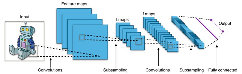
5.2.1 Convolutional Neural Networks(CNN)
The concept of time delay neural networks (TDNN) introduced by (Waibel et al.
[54]) is considered the precursor to the CNNs. TDNN is a feed-forward network
was basically introduced for the speech recognition. It has proved its efficiency
in handling a long temporal context information of a speech signal by its precise
hierarchical architecture, outperforming the standard DNN (Peddinti et al.[40]).
Attempts to customize TDNN for image processing tasks led to the CNNs. CNNs
as described in (Ketkar[27]) handle the input as matrix with two dimensions. This
property made this kind of DNN a perfect choice to process images where each image
is considered as matrix its entries are the pixels of this image. Basically, each CNN
consists of the following layers [27]:
• Convolutional layer
• Pooling layer
• Fully Connected Layer
The convolutional layer makes some kind of scanning over the input matrix to an-
alyze it and extract some features from it. In other words, some kind of window
sliding over the matrix where in each step a filter will be applied on this window
(this smaller part of input matrix). This process requires two parameters, the kernel
size (e.g 3*3) which denote to the size of this window or the size of this part from the
input will be filtered in each step. The second parameter is a step size which denotes
to the sliding size in each step. One could imagine this process as a filter with two
”small” dimensions moved over a big matrix, with a fixed sliding size, from left to
right and from top to bottom. The kind of so called P adding determines how this
filter should behave on the edges of the matrix. The filter has fixed weights that are
used together with the input matrix values in the current window to calculate the
result matrix. The size of this result matrix depending on the step size, the padding
way, and the kernel size. Usually contains the CNN two sequential convolutional
layers, each with 16 or 32 filter. The second one receive the result matrix of the first
layer as input. Then these two layers are followed with a pooling layer.
According to [27] the main role of pooling layer is to pass on only the most relevant
signal from the result matrix of the convolutional layers. So, it performs a kind of
aggregation over this matrix. For example the max pooling layer considers only the20 5. Deep Neural Networks
highest value in kernel matrix and ignores all other values. Pooling layer helps in
reducing the complexity in the network by performing an abstract representation of
the content.
Each neuron in the fully connected layer is connected to all input neurons and all
output neurons. This layer is connected to the output layer which has a number of
neurons equal the number of classes in the classification problem. The result layer
of convolutional and pooling layers must be flattened before it passed on to the fully
connected layer. Which means this layer receives the object features without any
position information (location independent).
The structure of CNN usually contains two sequential similar convolutional layers
followed by a pooling layer, after that again, two convolutional layers followed by a
pooling layer. Finally a fully connected layer, followed by the output layer. Figure
5.5 illustrates this structure.
Figure 5.5: Typical Convolutional Neural Network [55]
5.2.2 Recurrent Neural Networks(RNN)
The RNN is a special type of DNN has a recurrent neurons instead of normal feed
forward neurons. Recurrent Neuron has unlike normal neuron an extra connection
from its output to its input again. This feed back connection enables applying the
activation function repeatedly in a loop. In other words, in each repetition the
activation learns something about the input and be tuned accordingly. So, over the
time these activation represents some kind of memory contains information about
the previous input (Elman [16]). This property made the RNN perfect to deal with
sequential input data need to be processed in order such as sentences. Thus, RNN
were be considered the best choice for NLP problems. Figure 5.6 gives a graphical
representation of the recurrent neuron and RNN.
Figure 5.6: Recurrent Neural Network [46]
Where X = x1 ,...,xn is the input sequence and H = h1 ,...,hn represents the hidden
states vector. But, RNN has a big problem called the vanishing gradient problem
discussed in (bengio et al.[5]). This problem denotes to a drawback during the back5.2. Types of DNN 21
propagation training process over the time. It means that RNN either needs too long
time to learn how to store information over the time, or it fails entirely. (Hochreiter
and Schmidhuber [24]) solved this problem with their proposed Long short-term
memory (LSTM) architecture. LSTM overcome the training problems of RNN by
replacing the traditional hidden states of RNN with special memory cells shown in
figure 5.7. This memory cells unlike RNN could store information over the time and
enabled thereby extracting more contextual feature in the input data (Graves [19]).
According to [19], the following composite function calculates the output of LSTM
hidden layer:
it = σ(Wxi xt + Whi ht−1 + Wci ct−1 + bi ) (5.4)
ft = σ(Wxf xt + Whf ht−1 + Wcf ct−1 + bf ) (5.5)
ct = ft ct−1 + it tanh(Wxc xt + Whc ht−1 + bc ) (5.6)
ot = σ(Wxo xt + Who ht−1 + Wco ct + bo ) (5.7)
ht = ot tanh(ct ) (5.8)
Where σ is the sigmoid activation function, i the input gate, f is the forget gate and
o is the output gate. (for more details please see [19])
Figure 5.7: Long Short-term Memory Cell [19]
As improvement of LSTM Networks is the bidirectional LSTM (BiLSTM). The idea
of bidirectional RNN introduced by (Schuster and Paliwal [49]) was to invest the
future context besides the past context to improve the contextual futures extraction
process. In other words, the learning process in BiLSTM is performed not only from
beginning to the end of the sequential input but also in the opposite direction. So,
we have in this architecture two LSTM, one in each direction as shown in figure 5.8.
Figure 5.8: Bidirectional LSTM Architecture [46]22 5. Deep Neural Networks
5.3 Word Embedding Techniques
Word embedding is the process of mapping phrases or vocabularies into numerical
vectors. This mapping can be done randomly or with methods like Glove (Penning-
ton et al.[41]) and Word2Vec (Mikolov et al. [36]), where the distance between these
vectors in this case represents information about the linguistic similarity of words.
So, we talk here about a special information for each language. In this section we
give a brief overview about the two models of Word2Vec embedding method which
are continuous bag of word (CBOW) and Skip-gram [36]:
5.3.1 skip-gram
This model tries to learn the numerical representation of some words called target
words which are suitable to predict their neighboring words. The number of neigh-
boring words should be predicted is a variable and called a window size, but usually
is 4 (Mikolov et al. [37]). Figure 5.9 (right) illustrates the architecture of this model.
Where W(t) is a target word and W(t−2) , W(t−1) , W(t+1) , W(t+2) are the predicted
context words (assuming that the window size is 4).
Figure 5.9: The architecture of CBOW and Skip-gram models [36]
5.3.2 continuous bag of words (CBOW)
This model work exactly in the opposite way, it predicts one word from a given
context, instead of predicting the context words from a target word as in Skip-
gram. The context here could also be one word. This model is visualized in figure
5.9 (left).
We saw in the previous chapter how techniques like BOW only take into account
the occurrence of words in the text and their frequency, and completely ignore the
context information. In the case of CBOW and Skip-Gram, context is taken into
account when the words are represented, which means that closely related words
that usually appear in the same context would have a similar representation (similar
vectors). For example the names of animals or the names of countries or words like
”king” and ”queen”.Chapter 6
Methodology
In this section we describe the model architecture that we used in our experiments.
We started with a very simple RNN based model. We then moved to an LSTM-
based model in order to take the advantages of the LSTM over RNN described in
the previous chapter. As the attention mechanism could be very useful to improve
the achieved accuracy of a classification problem we then upgraded our model to an
bidirectional LSTM with self attention mechanism. We also introduced two hybrid
models we performed by adding some extra layers to these three baseline models in
order to achieve more classification accuracy. In the following we gave each model
a short name for simplicity.
6.1 Word-based recurrent neural Network (RNN):
This is simple model consists of the following layers:
• Input layer: This is simply an embedding layer used to map every word in
the input sentence to a numeric vector with random values. The dimension
of this vector will be tuned for each experiment separately depending on the
best achieved accuracy as we will see later.
• RN N layer: A bidirectional RNN architecture consisting of two hidden layers.
The number of units for each layer (hidden size) will be also tuned experimen-
tally.
• Output layer: Which is a linear function simply calculates the likelihood of
each possible class in the problem from the hidden units values of the previous
layer.
The mathematical structure for this model can be described as follows:
h(t) = fH (WGH x(t) + WH H h(t − 1)) (6.1)
y(t) = fS (WH S h(t)) (6.2)
Where WGH , WH H ,WH S are the weights between layers. x(t), y(t) represent the in-
put and output vector, respectively. fH represents the activation function of hidden
layers and fS the activation function of output layer.24 6. Methodology
6.2 Word-based Long-Short Term Memory (LSTM):
• Input layer: The same as the input layer for RNN
• LST M layer: An unidirectional LSTM architecture consisting of number of
hidden states as introduced the previous chapter 5. The number of these states
(hidden size) will be also tuned experimentally as for RNN.
• Output layer: The same as the output layer for RNN.
The mathematical structure for LSTM model is described in section 5.2.2
6.3 Bidirectional LSTM with self attention mech-
anism (biLSTM-SA):
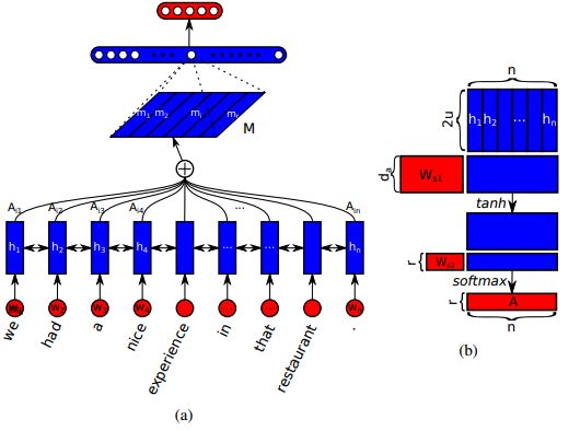
This model introduced by (Lin et al.[31]) consists of two main components, namely
biLSTM and a self-attention network. The first part (biLSTM) receives the embed-
ding matrix which contains the word-based numerical representation of the input
sentence and produce a hidden states matrix H, as we will see later. In order to
calculate the linear combination between the vectors of H, a self-attention mech-
anism would be applied many times on H considering different parts of the input
sentence. The structure of this model illustrated in Figure 6.1.
Figure 6.1: biLSTM with self-attention mechanism [31]
The following scenario clarifies the workflow of Figure 6.1 as described in [31]. As-
sume the input for the proposed model is a sentence consists of n words. First those
words will be mapped to a real value vectors (for our experiments we used random
embedding). So the output of this step will be a matrix represents the sentence S its
columns are those embedding vectors which mean S will have the size n*d. Where
d is the embedding size (The dimension of the embedding vectors).
S = (W1 , W2 , ...Wn ) (6.3)6.4. Hybrid model (CNN-biLSTM-SA): 25
Matrix S will be passed to a biLSTM represented in the following equation which will
reproduce and reshape S extracting some relationships between its columns(between
the words in the input sentence):
−
→ −−−−→ −−→
ht = LST M (wt , ht−1 ) (6.4)
←
− ←−−−− ←−−
ht = LST M (wt , ht−1 ) (6.5)
So, the produced hidden state matrix H has the size of n*2u where u is the hidden
size of the LST M in one direction.
H = (h1 , h2 , ...hn ) (6.6)
Now, to calculate the linear combination over the hidden state matrix H, the self-
attention in 6.7 will be applied on it. Where ws2 is a weight vector of size da and
Ws1 is a weight matrix of size da *2u and da is a hyper parameter. The output
a is a vector of values focus, according to [31] on one part of the input sentence.
But, the main goal is to obtain the attention over all parts of the sentence. So, the
vector ws2 in equation 6.7 is replaced by a matrix Ws2 of size r*da where r is also a
hyper parameter. Accordingly, the output will be a matrix A represents the applied
attention on r parts of the input sentence as in equation 6.8.
a = sof tmax(ws2 tanh(Ws1 H T )) (6.7)
A = sof tmax(Ws2 tanh(Ws1 H T )) (6.8)
After that the sentence embedding matrix M will be produced by multiplying the
hidden state matrix H with the weights matrix A as follows:
M = AH (6.9)
Finally, matrix M will be passed through a fully connected and output layer respec-
tively, to eliminate the redundancy problem.
6.4 Hybrid model (CNN-biLSTM-SA):
The model proposed in (Jang et al.[25]) for sentiment analysis problem inspired us to
add more component to the previous model (biLSTM-SA) in order to achieve better
accuracy. Authors in [25] proved that applying a convolution over the input vectors
lead to less dimensions in extracted features before it passed to LSTM which helps
it improve its performance. This reduction in dimensions is achieved because this
convolution according to [25] can extract some features from the adjacent words
in the sentence before it comes to the turn of LSTM to extract the long-short
dependencies. Accordingly, we added two 2D convolutional layers to the biLSTM-
SA model hoping to improve its performance. Each of those layers has a kernel
size of (3,3) and a stride of (2,2). Figure 6.2 gives a simplified illustration for the
structure of this model.You can also read