An Automated Approach On Generating Macro-Economic Sentiment Index Through Central Bank Documents
←
→
Page content transcription
If your browser does not render page correctly, please read the page content below
Imperial College London
                             Department of Mathematics

    An Automated Approach On Generating
   Macro-Economic Sentiment Index Through
          Central Bank Documents

Author:
Ruizhe Xia (CID: 01201752)

                         A thesis submitted for the degree of

                     MSc in Mathematics and Finance, 2019-2020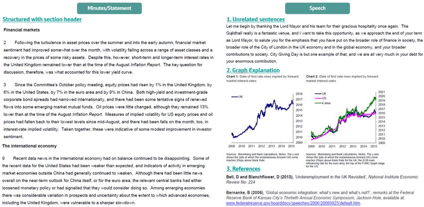
Abstract

I proposed an automated approach on creating region-specific dictionary to quantify central bank’s view on
macroeconomics and interest rate using documents including press conference scripts, monetary policy com-
mittee meeting minutes, member’s speeches and statements, which outperforms any other existing dictionary
and even the most recent FinBERT model [1] which contains more than 110 million parameters. This thesis
introduced an innovative way to label the document with positive/negative/neutral sentiment in order to con-
struct a new economical dictionary. This thesis demonstrated how the Latent Dirichlet Allocation1 [2] can be
applied as a language noise filter to remove the less relevant sentences. And this paper compared the dictionary
performance with two famous economic dictionaries of ’Financial Stability Dictionary’ and ’Loughran McDon-
ald Dictionary’, and proved that self-created dictionary is having better and consistent performance than the
existing dictionary. This paper also showed how the dictionary can work as a feature reduction method for
working with Machine Learning Models when the availability of documents is limited.

The goal is not only just to provide a quantitative way to interpret the economical meaning of central banks
documents, but also to show how the central bank sentiment is closely related to LIBOR rates. In this paper, I
will primarily demonstrate how the algorithm is applied to Bank of England materials, but the model is largely
applicable on all other major central banks, namely ECB and FED. In the fourth chapter of this thesis, I will
show hows the sentiment looks like on each central banks and its local rates.

The sentiment performance is also fairly promising. I trained the dictionary only on documents before 2009
to prevent looking forward bias. The final dictionary consists of only 293 words with 124 positive words and
169 negative words. And this dictionary still captures interest rate sentiment until 2020, by achieving 0.351
correlation with Sterling LIBOR 1Y rate. The performance is further validated by using the model train from
BOE onto other central banks’ documents, namely ECB and FED, where it still shows a correlation of 0.336
with their respective local LIBOR rates, comparing to 0.255 correlation for FS dictionary sentiment and 0.04
correlation on LM dictionary sentiment.

To further validate the performance of the model, I introduced the most recent financial NLP model, Finbert
[1], and proved that complicated models not necessarily outperform the simple model. The simple dictionary-
based sentiment based on filtered speech and minutes shows a better correlation with the LIBOR rate than the
Finbert sentiment. And finally, I introduce a new method to measure the predictive power of various sentiment
on various economical indices, including GDP, CPI, unemployment rate and interest rate, which validates the
strong connections between central bank documents’ sentiment and macro-economic conditions.

   1 Blei, David M.; Ng, Andrew Y.; Jordan, Michael I (January 2003). Lafferty, John (ed.). ”Latent Dirichlet Allocation”. Journal

of Machine Learning Research. 3 (4–5): pp. 993–1022. doi:10.1162/jmlr.2003.3.4-5.993. Archived from the original on 2012-05-01.
Retrieved 2006-12-19.
Acknowledgements

I need to appreciate Cissy Chan and many other people from BlackRock for guiding me through this project.
They did offer me lots of great insights and suggestion on text mining and the understanding of central bank
policies and languages. This thesis would not be possible without their patience and assistance in the past few
months.

And I also need to appreciate my supervisor Johannes Muhle-Karbe for the suggestions on modifying thesis
structures and on improving the explanations of various algorithms I implemented throughout the project.

And finally, I need to thank Stack Overflow, Wikipedia and Google for helping me debug my code and scripts.
Contents

1 Introduction                                                                                                                                                              2
  1.1 Literature Review . . . . . . . . . . . . . . . . . . . . . . . . . . . . . . . . . . . . . . . . . . . .                                                             2
  1.2 Project Overview . . . . . . . . . . . . . . . . . . . . . . . . . . . . . . . . . . . . . . . . . . . . .                                                            3
  1.3 Data . . . . . . . . . . . . . . . . . . . . . . . . . . . . . . . . . . . . . . . . . . . . . . . . . . . .                                                          6

2 Dictionary Based Model (Baseline)                                                                               7
  2.1 Existing Dictionary . . . . . . . . . . . . . . . . . . . . . . . . . . . . . . . . . . . . . . . . . . . . 8
  2.2 Region-specific Sentiment Algorithm . . . . . . . . . . . . . . . . . . . . . . . . . . . . . . . . . . 9
  2.3 Baseline Model Performance . . . . . . . . . . . . . . . . . . . . . . . . . . . . . . . . . . . . . . . 11

3 Semantic Language Cleaning                                                                                                                                               15
  3.1 What Is LDA . . . . . . . . . . . . . . . . . . . .      .   .   .   .   .   .   .   .   .   .   .   .   .   .   .   .   .   .   .   .   .   .   .   .   .   .   .   16
  3.2 LDA For Paragraph Clustering In BOE Minutes              .   .   .   .   .   .   .   .   .   .   .   .   .   .   .   .   .   .   .   .   .   .   .   .   .   .   .   18
  3.3 LDA For Language Filtering In BOE Speech . .             .   .   .   .   .   .   .   .   .   .   .   .   .   .   .   .   .   .   .   .   .   .   .   .   .   .   .   20
  3.4 Language Filtered Model Performance . . . . . .          .   .   .   .   .   .   .   .   .   .   .   .   .   .   .   .   .   .   .   .   .   .   .   .   .   .   .   22
      3.4.1 BOE Interest Rate Sentiment . . . . . . .          .   .   .   .   .   .   .   .   .   .   .   .   .   .   .   .   .   .   .   .   .   .   .   .   .   .   .   22
      3.4.2 BOE Topical Sentiment . . . . . . . . . .          .   .   .   .   .   .   .   .   .   .   .   .   .   .   .   .   .   .   .   .   .   .   .   .   .   .   .   24

4 Model Extensions                                                                                                                                                         27
  4.1 Multinomial Naive Bayesian Model . . . . . . . . . . . . . . . . . . . .                                 .   .   .   .   .   .   .   .   .   .   .   .   .   .   .   27
      4.1.1 What Is Multinomial Naive Bayesian Model? . . . . . . . . . .                                      .   .   .   .   .   .   .   .   .   .   .   .   .   .   .   27
      4.1.2 Bag-of-word And Why Dimension Reduction Is Needed? . . . .                                         .   .   .   .   .   .   .   .   .   .   .   .   .   .   .   28
      4.1.3 TF-IDF Weighting In Document Representation . . . . . . . .                                        .   .   .   .   .   .   .   .   .   .   .   .   .   .   .   29
      4.1.4 Multinomial Naive Bayesian Model Based On BOE Dictionary                                           .   .   .   .   .   .   .   .   .   .   .   .   .   .   .   30
  4.2 Cross Region Performance Validation . . . . . . . . . . . . . . . . . . .                                .   .   .   .   .   .   .   .   .   .   .   .   .   .   .   35

5 Performance comparing to other existing measures                                                                                                                         37
  5.1 Comparison With FinBERT Model . . . . . . . . . . . . .                      .   .   .   .   .   .   .   .   .   .   .   .   .   .   .   .   .   .   .   .   .   .   37
      5.1.1 What Is FinBERT . . . . . . . . . . . . . . . . . .                    .   .   .   .   .   .   .   .   .   .   .   .   .   .   .   .   .   .   .   .   .   .   37
      5.1.2 How To Calculate FinBERT Sentiment In Python                           .   .   .   .   .   .   .   .   .   .   .   .   .   .   .   .   .   .   .   .   .   .   38
      5.1.3 Why Choose FinBERT As Benchmark . . . . . . .                          .   .   .   .   .   .   .   .   .   .   .   .   .   .   .   .   .   .   .   .   .   .   39
      5.1.4 FinBERT Model Performance . . . . . . . . . . . .                      .   .   .   .   .   .   .   .   .   .   .   .   .   .   .   .   .   .   .   .   .   .   40
  5.2 Forecasting With Sentiment Indexes . . . . . . . . . . . .                   .   .   .   .   .   .   .   .   .   .   .   .   .   .   .   .   .   .   .   .   .   .   42

6 Possible future works                                                                                                                                                    46

A Full vocabulary of the dictionaries                                                                                                                                      47

B LDA Model details                                                                                                                                                        50

Bibliography                                                                                                                                                               54

                                                          1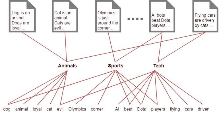
Chapter 1

Introduction

1.1     Literature Review
Sentiment analysis is a model that aims to extract sentiment, opinion or attitudes of people/institution from
written language, including but not limited to sentences, paragraphs, documents, social media. [3]. And nor-
mally there are two approaches regarding this task: (1) machine algorithms that extract features and sentiments
from texts with ’word count’ representation [4, 5, 6, 7], (2) deep learning-based algorithms that extract sen-
timents from texts which are represented by different types of embedding[8, 9]. The first methods are easy
to implement but suffer from its failure of ignoring semantic information based on the order of sequence or
dependency between different vocabularies. The second method is often required a huge amount of labelled text
data of the same context to learn its explosively large number of parameters.

In Natural Language Processing (NLP) community, there has been numerous successful development and
wide-spread discussion on language model and text classification, but it was majorly focused on conversational
language rather than financial and economical language. And the majority of successful NLP models were
trained on a huge amount of text data, which is highly impossible in our scenarios. (At least hundreds of thou-
sands labelled sentences on economical content to train the over 100 million parameters in different NLP model)
Take one example of the very recent successful language model was the ”BERT: Pre-training of Deep Bidirec-
tional Transformers for Language Understanding” published by researchers at Google AI Language, which was
pre-trained with over 110 million parameters. Contrasting to the popularity and fast evolutions of generic NLP
models (BERT 2018, XLNET 2019, GPT3 2020), researches and developments in language model on financial
texts, especially on macro-economics topics, seems to be stagnated and less popular. The main reason that
to pre-train an accurate Bert model would require millions of economical documents which is generally not
available for most of researchers.

One of the very first language model on financial context was developed by Loughran and McDonald (2011)
”When Is a Liability Not a Liability? Textual Analysis, Dictionaries, and 10-Ks”[7] in understanding the tones
of 10-Ks, suggesting that the contextual sentiments of same words could be significantly different in different
text sources. And further proven by the 2017 paper ”Sentiment in Central Banks’ Financial Stability Re-
ports”[6], they suggest the financial stability dictionary based on Federal reserve communication is 30%different
to dictionary created by Correa, Ricardo, Keshav Garud, Juan M. Londono, and Nathan Mislang (2017) which
is based on US public listed companies’ annual reports. Hence, the language model should need to be re-trained
based on the specific context before any forecasting/classification purposes.

There have been several papers talking about central banks communication and deriving sentiments, but most
of the papers were using the news data-set, such as Dow Jones Newswires[10] and Factiva dataset[11], to look
at central bank communication rather than looking at the central bank documents directly. And most of the
paper simply using the existing dictionary rather than creating task-specific dictionary. The 2015 paper ”Does
Central Bank Tone Move Asset Prices?”[12] looked at ECB press conferences held after ECB policy meeting.
And they proved the changes in ECB tine convey generic information for stock markets as well as views of future

                                                       2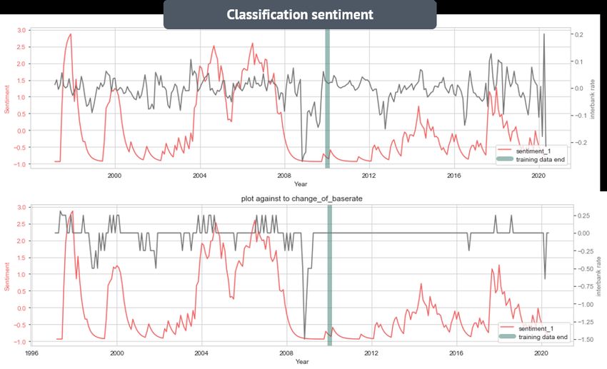
monetary policy. The May 2020 Paper, ”Making text count: economic forecasting using newspaper text”[13],
had used 10 different dictionary-based sentiment indexes for forecasting macroeconomics movement, including
Financial Stability dictionary, Loughran and McDonald dictionary, social media sentiment dictionary1 , Harvard
IV psychological dictionary, Anxiety and Excitement dictionary2 , Economic Uncertainty3 , Monetary Policy
Uncertainty4 and Economic Policy Uncertainty dictionary5 . And the financial stability dictionary has been the
best-performed dictionary [13] correlated with various indicators including ”OECD UK business confidence”,
”Lloyds Business Barometer” and ”Composite PMI”, in term of size of error between predicted and actual
financial indicators. In my research, I will focus on comparing the performance of Financial stability dictionary
as my baseline model.

There has also been limited research on the sentiment of central bank minutes, speech and statements. We
would expect that the communication of central banks reveals their opinions on short-term and long-term macro-
economic movements, such as the interest rate movement and LIBOR rates. The 2019 paper of ”Narrative
monetary policy surprises and the media” [14] reveals a significant information-surprise on various topics after
the central bank documents being published, including interest rate, risk, uncertainty and growth. Both ”Mea-
suring Central Bank Communication: An Automated Approach with Application to FOMC Statements”[15]
and ”Between hawks and doves: measuring central bank communication ”[16] and proved significant relation
between central bank document sentiment index and treasury bills returns and interest rates. Hence, it is the-
oretically feasible to generate sentiment index based on central bank documents, while greatly reflects banks’
opinions and predicts on economical and financial indicators’ movements.

1.2      Project Overview
Natural language processing on central bank documents has always been a challenge because of the limited
documents available. The popular deep learning model such as XLNET and BERT requires at least hundreds
of thousands of labelled document which is very unlikely to be available. It is because all the latest NLP
language models are having hundreds of millions of parameters6 . (And in this thesis, I will also show that my
model outperforms the most recent FinBERT model [1] on interest rate prediction tasks.) Bank of England
(BOE) usually post one minute per month and 3 speech per month. This means I was working with only 1044
documents starting from 1997 to 2020 to train a decent language model. This is also the reason why there
are limited researches on the central bank minutes and speeches directly, and why most of the financial NLP
papers are working with news database or cooperate finance documents. But this also makes me curious about
how much information can be extracted from the central bank documents and on how well it will perform on
explaining and forecasting the movement of various financial indexes. (eg: LIBOR, GDP, Unemployment rate)

In this project, the main motivation is to understand how interest rate sentiment can be extracted from central
bank communication documents and how well the language model could perform despite the constraints on
data availability. I decided to take the challenge to automate a sentiment generation process to quantify the
central bank’s view on the macroeconomic situation and establish a link to existing financial and economical
indexes. Because of limited data availability, I intentionally decided to take some simple model on extracting
sentiments out of BOE minutes and speeches, such as dictionary-based model and Multinomial Naive Bayesian
model, instead of a deep-learning-based model.
   1 Finn Årup Nielsen, 2011, ’A new ANEW: Evaluation of a word list for sentiment analysis in microblogs’,

https://arxiv.org/abs/1103.2903
   2 Rickard Nyman, Sujit Kapadia, David Tuckett, David Gregory, Paul Ormerod and Robert Smith, ’News and narratives in

financial systems: exploiting big data for systemic risk assessment’, https://www.bankofengland.co.uk/working-paper/2018/news-
and-narratives-in-financial-systems
   3 Michelle Alexopoulos Jon Cohen, 2009. ”Uncertain Times, uncertain measures,” Working Papers tecipa-352, University of

Toronto, Department of Economics
   4 Husted, Lucas, John Rogers, and Bo Sun (2017). ”Monetary Policy Uncertainty”. International Finance Discussion Papers

1215. https://doi.org/10.17016/IFDP.2017.1215
   5 Scott R. Baker, Nicholas Bloom, Steven J. Davis, Measuring Economic Policy Uncertainty, The Quarterly Journal of Economics,

Volume 131, Issue 4, November 2016, Pages 1593–1636
   6 BERT base has 12 layers (transformer blocks), 12 attention heads, and 110 million parameters. BERT Large has 24 layers, 16

attention heads and, 340 million parameters. XLNet has 24-layer, 1024-hidden, 16-heads, 340M parameters. GPT-2 has 1.5 billion
parameters

                                                               3
And Latent Dirichlet allocation (LDA)[2] has been a famous and successful probabilistic method in discover
topics from a set of documents [17]. LDA assumes each document has a probability distribution over different
topics, and each topic has a probability distribution over different vocabularies. So based on the words that
occurred in the text, the LDA model could give a probability distribution over different topics for this text
(either sentences, paragraphs or documents). You can understand more about LDA at Section 3.1. But in
this thesis, I aim to use LDA for two purposes: (1) cluster paragraphs in minutes into 6 different topics (2)
semantically clean up the language of speeches by removing semantic incoherent sentences in the speech.

This thesis contributes to macro-economic sentiment construction consist of two parts:

  1. By learning a new interest-rate dictionary based on the Bank of England documents, the dictionary-based
     sentiment that constructed on BOE minutes and speeches can capture the bank’s opinion and sentiment
     on the current macro-economic level. And the sentiment constructed is having a strong connection with
     UK based rate and LIBOR rate movement. But the same methodology can easily be applied to other
     banks. I will also demonstrate how well the sentiment constructed on FED and ECB documents are
     closely connected to their local LIBOR rate, in addition to BOE documents.

  2. Innovative using Latent Dirichlet allocation (LDA) (see Section 3.3 for more details) as language style
     filter to remove less relevant sentences in BOE speech and only keep relevant sentences that have similar
     language style as BOE minutes. This semantic language cleaning significantly improved the dictionary-
     based model performance.

To construct the sentiment index on UK, I first build up web scraper on BOE websites to download all the 1044
files available. Then I use the document from 1997-2009 as the training data, the documents starting 2010 are
viewed as testing data (out-of-sample documents) to validate the consistency of performance. The label of the
document is based on if there is a local risk rise or drop within the next 6 months after the document published.
In this case, if UK base rate increases within the next 6 month, the document is label as positive sentiment
document. If UK base rate drops within the next 6 month, the document is labelled as negative sentiment
document. And if neither things happen, the document is then labelled as neutral sentiment document.

Then I assume the work with positive sentiment will appear more frequently in positive sentiment documents
and vice versa. The dictionary was then selected based on the possibility of document being positive/negative
given this word appeared. After the dictionary was trained, the sentiment of each document was calculated by
looking at the difference between positive and negative scores divided by the sum of the positive and negative
score. And the UK interest rate sentiment was constructed by averaging all texts published in the same month,
and exponentially moving averaged with past 3 months interest rate sentiment. And the final dictionary-based
sentiment is classified as interest rate sentiment in the next month. I quantify the sentiment performance by
looking at the correlation between sentiments and Sterling LIBOR 1Y rate.

But I found the dictionary-based method applied on minutes was consistent, but performance on speech was
horribly performed with 0.3 correlation on training data but 0 correlation on testing data. Hence, I innovative
used Latent Dirichlet allocation (LDA) to remove the noise in BOE speech and the performance improve sig-
nificantly. And the final dictionary size is 294 words with 124 positive words and 169 negative words. And the
dictionary performance is significantly better than sentiment constructed based on ’Financial Stability Dictio-
nary’ and ’Loughran McDonald Dictionary’.

                                                       4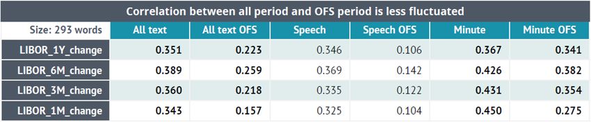
Figure 1.1: Sentiment index created by the final model and plotted against UK LIBOR 1Y rate and base rate

In addition, I talked about two model extensions. I first went one step forward to build work embedding on
these 294 words and constructed a multi-nominal Naive Bayesian model to better indicate possible base rate
movements. But the main take away is that the dictionary construction method proposed in this thesis can act
as a feature selection algorithm for different NLP tasks. And I secondly applied the same methodology on FED
and ECB documents and achieved still achieve high correlation with those local interest rate. This validates
the economical meaning and performance of the model even further.

And finally, I introduced the most recent and powerful pre-trained model FinBERT and compared its perfor-
mance with my UK interest rate dictionary sentiment. And I showed that my model actually performed better,
in term of both speed and accuracy, than the FinBERT model that has 110 million parameters. And I also
introduced new metrics rather than correlation to validate that my model carries the highest amount of new
information on interest rate prediction tasks than many other algorithms and existing indexes.

                                                     5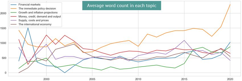
1.3     Data
All data used in this thesis are all publicly available. Those data are either downloaded directly from the
web-page or download by the web-scraper developed by myself. But I will not discuss how the web-scraper was
constructed in this thesis because this is not very relevant. I only downloaded minutes and speeches from central
bank official website and ignoring other documents at the current stage. And the documents downloaded are
unlabelled, and hence adding an automated and accurate document label is an essential step in this project.

For more details of the data sources:

  1. Bank of England speech:
     https://www.bankofengland.co.uk/news/speeches
  2. Bank of England minute:
     https://www.bankofengland.co.uk/news/news
  3. The Federal Reserve minutes:
     https://www.fedsearch.org/fomc-docs/search?advanced search=true&from year=1997&search precision=
     All+Words&start=0&sort=Relevance&to month=7&to year=2020&number=10&fomc document type=
     minutes&Search=Search&text=&from month=3
  4. European Central Bank Press Conference:
     https://www.ecb.europa.eu/press/pressconf/html/index.en.html
  5. European Central Bank Monetary policy accounts:
     https://www.ecb.europa.eu/press/accounts/html/index.en.html
  6. LIBOR 1Y 6M 3M 1M rate:
     https://fred.stlouisfed.org/series/EUR12MD156N
  7. UK base rate, FED base rate, ECB base rate are easily found on their respective central bank website

And here is the summary on the text data I am using in this project

                                  Number of document          Word Count after cleaning          Date range
   Bank of England minute                783                           2200                       1997-2020
   Bank of England speech                261                           2080                       1997-2020
  The Federal Reserve minute             324                           3868                       1997-2020
     ECB policy accounts                  45                           3644                       2015-2020
  ECB policy press conference            240                            837                       1998-2020
       Table 1.1: Descriptive statistics of downloaded documents from 4 different major central banks.

Noted that the table above only includes the articles after I removed all the non-relevant, repeated documents.
So if you build the web-scraper using the address above, you may download a much higher amount of documents
that the number stated here. I have applied a filter on the title to make sure this document is either shared by
the Monetary Policy Committee or explaining the reasons behind the macro-economic policy movement.

                                                       6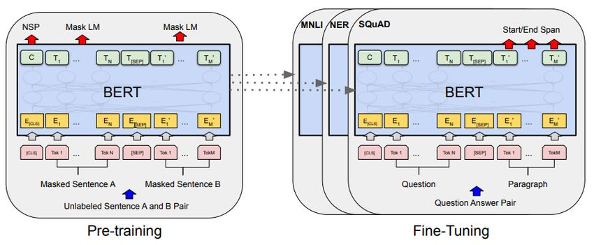
Chapter 2

Dictionary Based Model (Baseline)

For the most of the time, the evaluation of text documents is through the subjective measure. From the text-
book articles we read in our school time, to the news articles, economics documents or even academic papers,
people’s understanding of those articles could be different from each other. And when people read the same
articles at different time and occasions, they might have a slightly different understanding of the sentiments
and the implications in the text documents. And the evaluation of the sentiments in the text documents can be
time-consuming as well as being inconsistent. Using an automated approach, such as sentiment dictionary on
specific contents (such as economical, political or conversational), could give a more objective evaluation of the
document, and we could perform a direct comparison on sentiments between documents published at different
times from different authors. And such sentiment constructed on documents can remove the inconsistencies
from the viewer’s personal opinion and experiences. A sentiment index is only meaningful when the sentiment
is generated from the consistent and objective evaluation.

In this section, I will first talk about the existing financial or economical dictionary, explain how to construct
document sentiment based on these two dictionaries as well as quantify their performances. After that, I will
introduce the method to generate document labels and to constructed a new region-specific economical dictio-
nary. And final I will compare the performance of this newly created dictionary with existing measures.

In term of the document I was working with, I have downloaded files from the website of Bank of England (BOE),
The Federal Reserve (FED) and European Central Bank (ECB)from 1997 to 2020. There are 783 BOE Speech,
261 BOE minutes, 285 ECB minutes, and 324 FED minutes. I will skip the details of web scraping in this paper.

But before the document can be used for any quantitative algorithm, we need to pre-process the document
through the process of:

   1. Remove documents that were too short, which carries limited information and would create bias in the
      sentiments. (Less than 100 words)
   2. Remove punctuation, hyperlinks, references, footnotes, HTML tags, special non-Unicode characters, num-
      bers and mathematical equations
   3. Set all characters into lower cases
   4. Remove the phrases and convert each word into is the base form, in another word, stemming and lemma-
      tization1
   5. Remove all the stop words (e.g. for, very, and, of, are, etc) which was chosen from famous NLTK word
      list proposed by Bird and Loper in 20042 .
   1 Stemming usually refers to a crude heuristic process that chops off the ends of words in the hope of achieving this goal

correctly most of the time, and often includes the removal of derivational affixes. Lemmatization usually refers to doing
things properly with the use of vocabulary and morphological analysis of words, normally aiming to remove inflectional end-
ings only and to return the base or dictionary form of a word, which is known as the lemma. For more details, please refer to
https://nlp.stanford.edu/IR-book/html/htmledition/stemming-and-lemmatization-1.html
   2 Natural Language Processing with Python – Analyzing Text with the Natural Language Toolkit, Steven Bird, Ewan Klein,

and Edward Loper, 2004, https://www.nltk.org/book/

                                                             7
Below shows the example of documents before and after the pre-processing.
Figure 2.1: Document before and after preprocessing
2.1 Existing Dictionary
word sentiment word sentiment
Abandon Negative Able Positive
Abdicating Negative Abnormally Negative
Abnormal Negative Abrupt Negative
Able Positive Absorb Positive
Abundance Positive Absorbed Positive
Acclaimed Positive Absorbing Positive
Table 2.1: LM Dictionary Table 2.2: FS Dictionary
There are two existing dictionaries I will discuss: Loughran and McDonald 2011, and Financial Stability dic-
tionary. Both of the dictionaries classify some word as positive sentiment words and some words as negative
sentiment words. LM dictionary consists of 229 words and was trained on 50115 pieces of listed firms annual
reports from 1994 to 2008. The FS dictionary consists of 391 words and was trained on 982 financial stability
reports of 62 countries, ECB, and IMF published between 2000 and 2015.
To calculate the sentiment of a document, we need to first convert vocabulary in both dictionaries to nor-
malised form by Stemming and Lemmatization. For example, the words from LM dictionary ”ABAN-
DON”, ”ABANDONED”, ”ABANDONING”, ”ABANDONMENT”, ”ABANDONMENTS”, ”ABANDONS”
are all converted to the same word ”abandon”. Then the document sentiment based on LM or FS dictionary is
simply:
#P − #N
Sentiment of Document =
#P + #N
where #P represents the sum of the frequencies of all positive vocabularies from LM/FS dictionary that showed
up in the document and #N represents the sum of the frequencies of all negative vocabularies showed in the
document. Hence words were neither negative nor positive are ignored. And there is no difference between
negative words and very negative words. (This drawback will be solved in the next section)
The final monthly central bank sentiment index is constructed by first averaging all texts published in the
same month (eg: May). Then it is exponentially moving averaged with half-life equalling 3 month3 . The final
sentiment is classified as the sentiment for next month (eg: June)
If I apply the above methods based on LM dictionary or FS dictionary on 1044 Bank of England documents,
I create LM sentiment and FS sentiment respectively. According to the method I set up the document label,
the sentiment should optimally go down when the central bank has a more pessimistic view on the macro-
economics, and the sentiment should optimally go up when the central bank has a more optimistic view on the
macro-economics. And the optimistic/pessimistic view can be validated by observing either a rate cut or a rate
hike in the next few months to control inflation or to boost the economy.
3 The choice of 3 months was based on maximising the constructed sentiment’s correlation with LIBOR 1Y monthly change
8Figure 2.2: LM dictionary sentiment on BOE documents and UK base rate change
Figure 2.3: FS dictionary sentiment on BOE documents and UK base rate change
The Figure 2.2 shows the sentiments generated from LM dictionary. And as you may observe, even though the
sentiment reflects the 2008 financial crisis as there is a significant drop in sentiment value from 2008 to 2009,
LM sentiment in the rest of the periods are merely noise as it failed to explain any rate hike or rate cut in the
past 20 years.
The Figure 2.3 shows the sentiments generated from FS dictionary. And as you may observe, the financial
stability dictionary is actually performing well in term of explaining the interest rate movement. We not only
observe the significant sentiment drop during the 2008 financial crisis, but also observe the significant sentiment
drop in 2012 European Financial Crisis, 2016 Brexit. And all the sentiment drop in 1998, 2002, 2008, 2016 are
followed by a series of rate cut in the next few months.
Hence, I observe that financial stability dictionary does have the explanatory power on reflecting the macro-
economic performance. So I decided to include some of the words from the Financial Stability dictionary into
my self-created BOE interest rate dictionary.
2.2 Region-specific Sentiment Algorithm
To construct a Bank of England interest rate dictionary and derive the sentiment index:
Step 1: Create BOE documents label based on UK base rate
The document download from the website does not have any labels in nature. And normally it would require
economic experts to read the documents and judge when this document (minute/speech) is carrying positive
and negative sentiment towards the macro-economic situation. However, this is not feasible in my projects and
there are 1044 documents for Bank of England alone. And much more are awaiting if includes ECB and FED.
9As a result, the document in this thesis is labelled based on local base-rate movement — if there is a base rate
rise or drop within the next 6 months after the document published. In this case, if the UK base rate increases
within the next 6 month, the document is label as positive sentiment document. If UK base rate drops within
the next 6 month, the document is labelled as negative sentiment document. And if neither things happen,
the document is then labelled as neutral sentiment document. The rationale is that the base rate has a strong
connection with the macro-economical situations. Usually rate cut represents the bank is boosting the economy
as the macroeconomic is not good enough as expected. And rate-hike represents the bank is controlling inflation
and overheating in the economy, hence macro-economics are performing well.
Figure 2.4: Label of the document against the dates of the documents being published
Finally, I split the BOE documents into in-sample and out-of-sample periods. In-sample documents are doc-
uments published before 2009-12-31, Out-of-sample (OFS) text are documents published after 2010-01-01. I
trained a dictionary based on in-sample and check performance based on OFS documents.
Step 2: Create Co-occurrence matrix on in-sample documents
After the documents being labelled, I calculated the number of times each word occur in a positive/negative/neu-
tral sentiment document that was published before 2009-12-31. Then for each word, for all sentiment-carrying
document that contains this word, I calculated the percentage of positive sentiment documents among all doc-
uments containing this word. Then the word is labelled as a positive sentiment word if it shows up more
frequently in positive sentiment documents than negative sentiment documents. And vice versa for detecting
negative sentiment words.
Figure 2.5: Word co-occurrence matrix with labelled documents
’negative count’ represents the number of negative sentiment documents that contain this word.
’positive count’ represents the number of positive sentiment documents that contain this word.
’neutral count’ represents number of no-sentiment documents that contain this word.
’p percentage no neutral’ represents the percentage of document being positive sentiment among all sentiment-
carrying documents that contain this word.
10’n percentage no neutral’ represents the percentage of document being negative sentiment among all
sentiment-carrying documents that contain this word.
Step 3: Select words into dictionary
The BOE dictionary is created based on the parameter space of (N, Ppositive , Pnegative , Mpositive , Mnegative ):
1. We include positive sentiment word into our ”BOE dictionary” by the criteria of:
(a) Showed up in at least N pieces of in-sample documents
(b) ’p percentage no neutral’ is greater than Ppositive
(c) After sorting on ’p percentage no neutral’, we select maximum Mpositive words into dictionary
2. We include negative sentiment word into our ”BOE dictionary” by the criteria of:
(a) Showed up in at least N pieces of in-sample documents
(b) ’n percentage no neutral’ is greater than Pnegative
(c) After sorting on ’n percentage no neutral’, we select maximum Mnegative words into dictionary
3. We include some words from FS dictionary into our ”BOE dictionary” by the criteria of:
(a) Positive Sentiment in FS dictionary and positive sentiment in word co-occurrence matrix
(b) Negative Sentiment in FS dictionary and negative sentiment in word co-occurrence matrix
And I finalised the parameter by optimising the classification accuracy based on in-sample documents:
1. Set-up grids for each of the parameter of (N, Ppositive , Pnegative , Mpositive , Mnegative ). In this my case,
I choose N from [30,50,70], P from [0.55,0.60,0.65] and M from [80,100,120]
2. For each set of parameter, construct the dictionary according to the method above
3. For each document, the document is calculated as a negative document if it contains more negative words
than positive words, according to the dictionary produced in the last step, and vice versa.
4. For each dictionary constructed, get the classification results for all in-sample documents, using the method
in the last step, and calculate the accuracy rate when comparing to the document label created in step 1.
5. Pick the set of parameters that generates the most accurate classification result. In my case, my final
dictionary has the parameter of (50,0.55,0.55,100,100)
Step 4: generate BOE dictionary sentiment index
To generate sentiment for each document:
1. Positive score: Sum of ‘p percentage no neutral’ for all positive words occurred in this document
2. Negative score: Sum of ‘n percentage no neutral’ for all negative words occurred in this document
3. Document Sentiment: (Positive score – Negative score) / (Positive score + Negative score)
Step 5: Monthly index by exponentially weighted averaging
The final monthly central bank sentiment index is constructed by first averaging the sentiments of all texts
published in the same month (eg: May). Then it is exponentially moving averaged with half-life equalling 3
months. The final sentiment is classified as the sentiment for next month (eg: June)
2.3 Baseline Model Performance
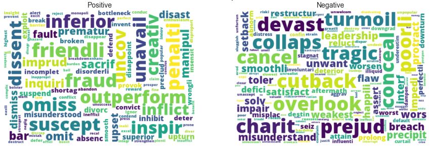
Figure 2.6 shows how does the dictionary looks like. The left includes words that are positive sentiment and
right includes words of negative sentiments. The size represents the value of ‘p percentage no neutral’ or ‘n
percentage no neutral’. The bigger the word is, the more import this word is in determine the sentiment of
documents. We could see that positive word includes: ”our-perform” ”friendly” ”superior”, and negative words
include: ”turmoil” ”collapse” ”misunderstand” ”cutback” ”breach”. There are noise and classification of the
words, but it largely represents the connection of each word to positive and negative sentiment words.
11Figure 2.6: Word cloud of BOE interest rate dictionary
Figure 2.7: Newly created dictionary sentiment on BOE documents and UK base rate change
Figure 2.7 shows how does the sentiment index using the Region-specific Sentiment Algorithm on raw
BOE document looks like4 , plotting against the base rate change from 1997-2020. The green line represents
the date where the training periods ends, and the sentiment on the right of green line are generated based on
the testing dataset. We could observe that for in-sample periods (left to green line), then sentiment increases
drastically when there is going to be a rate hike and drop to -1 when there is going to be a rate drop. However,
after the training period end (OFS, right to green line), the fluctuation of the sentiment index becomes smaller
and less meaningful. We did not observe a drop in 2016. Hence, we could say implementing the algorithm
directly does not work well as the language in the documents is changing. The sentiment important word in
1997-2010 is different from sentiment determining word after 2010. We definitely need some algorithm to clean
up the language in the documents and make a dictionary-based model can work well across all time.
4 I said ”raw document” because I use the document directly after pre-processing. In the next section, I will introduce the
method to clean up the language of documents and improve the performance
12Figure 2.8: Correlation between sentiment based on different dictionaries with the monthly change ratio of
different Sterling LIBOR rate, including LIBOR 1Y, 6M, 3M and 1M rate.
But if we zoom out for now and comparing the sentiment performance across different dictionary, the Figure
2.8 shows the correlation between sentiments created by different dictionaries and monthly change of LIBOR
1Y 6M 3M and 1M rate. For more information about each column:
All text: represent sentiment from 1997 to 2020, created based on both UK minutes and speech before 2010
All text OFS: represent sentiment from 2010 to 2020, created based on both UK minutes and speech before
2010
Speech: represent sentiment from 1997 to 2020, created based on both UK speech only before 2010
Speech OFS: represent sentiment from 2010 to 2020, created based on both UK speech only before 2010
Minute: represent sentiment from 1997 to 2020, created based on both UK Minute only before 2010
Minute OFS: represent sentiment from 2010 to 2020, created based on both UK Minute only before 2010
Hence for example, in the first table, the value of 0.028 in the top left entry represents the correlation between
{sentiment index created by LM dictionary from 1997 to 2020 created based on both minute and speech} and
{UK Libor 1Y monthly change from 1997 to 2020} is 0.028. And from these three tables, we could achieve the
following conclusions:
1. Context is important for dictionary based model
LM dictionary barely captures any useful sentiments in the central bank statements as its sentiment has almost
0 correlation on all types of LIBOR rate and documents. The FS dictionary, in contrast, has 0.278 correlation
with LIBOR 1Y rate based on both minutes and speech. And our BOE dictionary constructed a sentiment with
0.351 correlation with LIBOR 1Y rate, especially on Bank of England Minutes. The difference in performance
is expected. LM dictionary is trained on US equity firms annual report, FS is trained on Central Bank financial
stability report and our dictionary is trained on BOE interest rate documents directly.
132. Minutes has consistent language styles over time
Both Financial Stability dictionary sentiment and self-created dictionary sentiment based on raw BOE docu-
ments have a consistent correlation with Libor 1Y rates. For self-created dictionary based on BOE minutes, it
has 0.387 correlation during the full sample periods and 0.344 during the out-of-sample periods with LIBOR 1Y
rate. And the same thing happens to the correlation with LIBOR 6M 3M and 1M. We could see the dictionary
that was created based on the document until 2009 still have large explanatory power on minutes until 2020.
This shows that the vocabulary used in BOE minutes are most of the time similar and unchanged over time.
3. It is harder to capture sentiment on speech
All three dictionaries perform significantly worse after 2009/12/31, and our own model performance completely
vanished after the training period. In all three tables, the ”Speech OFS” is almost 0 for all dictionaries and all
different LIBOR rates. This shows the important word in 1997-2010 is different from the important words from
2010-2020. This could due to the change in language in the speech, whereas the performance of minutes was
fairly consistent. This also proves that the language of speech changes significantly over time. The speakers
tend to use different vocabularies and different way to speak in different years.
4. Performance slightly varies across different LIBOR rate:
Generically speaking, the model performs the best on LIBOR 6M, which is understandable that the document
is labelled based on whether is rate change in the next 6 months. But the correlation to different LIBOR is not
significantly different from each other.
14Chapter 3
Semantic Language Cleaning
From the previous part, we could judge the consistency of the language by looking at how quick the performance
of the dictionary decays in the out-of-sample period. We observe that BOE minutes are consistently well-
performed, while the speeches sentiment has a very bad correlation with LIBOR rate during OFS periods. And
if you look at the speeches and minutes directly, we could also observe that the language is consistent cover
time in minutes while inconsistent overtime in speech.
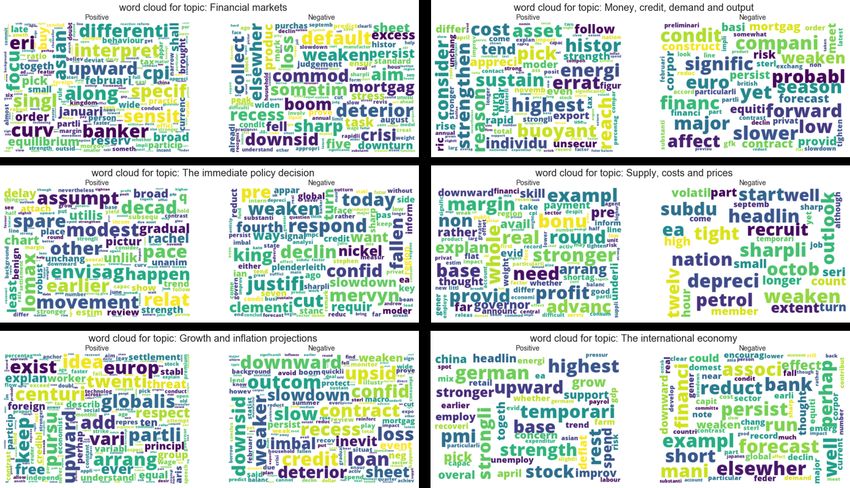
Figure 3.1: Comparison between minutes and speech
As you may observe from the above chart, you could see that the language is standard and consistent for the
Bank of England minutes. It has standard header name for each section, which indicates the topics of each
paragraph. And the header names are highly similar through the past 23 years from 1997 to 2020. It always
talks about inflation, credit, demand/supply and other topics in macroeconomics. But the language in speech is
inconsistent and noisy. It contains texts of different format: graph, equations, references, report and unrelated
sentences. And the topics changes over time as speech covers more about recent news and less economic contents.
Hence extra actions are needed to clean up the language in documents, to improve the performance of sentiment
model. And in this paper, I decide to use Latent Dirichlet Allocation (LDA) topic modelling to remove the less
relevant sentences in speech.
153.1 What Is LDA
Latent Dirichlet Allocation (LDA) is a “generative probabilistic model” of a collection of composites made up
of parts. Its uses include Natural Language Processing (NLP) and topic modelling, among others. The context
of population genetics was proposed by J. K. Pritchard, M. Stephens and P. Donnelly in 200012 . And LDA was
applied in machine learning by David Blei, Andrew Ng and Michael I. Jordan in 20033 .
Intuitively speaking, LDA is a form of unsupervised machine learning algorithm that find topics in documents
automatically, a probabilistic clustering algorithm. Each document can be described by a distribution of topics
and each topic can be described by a distribution of words. The LDA topic model assumes:
1. Documents exhibit multiple topics
2. A topic is a distribution over a fixed vocabulary
3. Only the number of topics is specified in advanced
4. All documents are assumed to be generated by generative process:
- Random choose a distribution over topics
- For each word in the document:
- Randomly choose a topic from the distribution over topics
- Randomly choose a word from the corresponding topic (distribution over the vocabulary)
According to the original paper[2], mathematically speaking, if I have a set of D documents, each document
having N words, where each word is generated by a single topic from a set of K topics. Hence mathematically,
we define dth document is a sequence of N words: wd = (wd,1 , wd,2 , ..., wd,N ). For example, if wd,1 = 3, this
represent in dth document, the word with id=1 show up 3 times. And the generative process above can be
mathematically written by that, for each document wd in corpus D, it is generated by for d = 1 : D:
1. We define the number of word N ∼ Poisson(ξ), but this is usually prefixed and no need to calibrated
2. We define the variable θ ∼ Dir(α)
3. Then in each word in the document wd,n :
(a) The topic is first chosen by zd,n ∼ Multinomial (θ). where θ is a k-dimensional Dirichlet random variable
(b) Given the chosen topic zd,n , we now assign a value to wd,n from a multinomial probability p (wn | zd,n , β)
4. By completing the loop above, we could now finally generate the document in the vector form wd =
(wd,1 , wd,2 , ..., wd,N )
Figure 3.2: Graphical representation of document generation process. The shaded circle is the final document
we generated. In LDA, we assume all document are generated by such process.
The Figure 3.7 visualize the generate process into plot. And mathematically, we can describe the document
as following joint distribution:
K
Y D
Y N
Y
p (β1:K , θ1:D , z1:D , w1:D ) = p (βi ) p (θd ) p (zd,n | θd ) p (wd,n | β1:K , zd,n )
i=1 d=1 n=1
1 Pritchard, J. K.; Stephens, M.; Donnelly, P. (June 2000). ”Inference of population structure using multilocus genotype data”.
Genetics. 155 (2): pp. 945–959.
2 Falush, D.; Stephens, M.; Pritchard, J. K. (2003). ”Inference of population structure using multilocus genotype data: linked
loci and correlated allele frequencies”. Genetics. 164 (4): pp. 1567–1587.
3 Blei, David M.; Ng, Andrew Y.; Jordan, Michael I (January 2003). Lafferty, John (ed.). ”Latent Dirichlet Allocation”. Journal
of Machine Learning Research. 3 (4–5): pp. 993–1022.
16−β1:K are the topics where each βk is a distribution over the vocabulary
−θd are the topic proportions for document d
−θd,k is the topic proportion for topic k in document d
−zd are the topic assignments for document d
−zd,n is the topic assignment for word n in document d
−wd are the observed words for document d, and this is the only observable variable
−α and η are the parameters of the respective dirichlet distributions
Parameter Estimation:
Given the Wd,n we could observe for d = 1 : D n = 1 : N , we want to estimate the following parameter during
the training process:
−βk : distribution over vocabulary for topic k
−θd,k : topic proportion for topic k in document d
−α : Distribution related parameter that governs what the distribution of topics is for all the documents in the
corpus looks like
−η : Distribution related parameter that governs what the distribution of words in each topic looks like
One common technique is to estimate the posterior of the word-topic assignments, given the observed words,
directly using Gibbs Sampling. More details of Gibbs Sampling for LDA can be found here4 . It took the original
Arthur 15 pages to solve the above equations and mathematically explain how LDA is assigning each document
into different topics and assign each topic to different words. As my thesis was not really focused on those
theories, but rather about how to implement and use them, I will skip the proof process.
But in term of how to implement it, we can intuitively understand it like that: after the parameter being
estimated after training on a set of documents, we could let LDA model describe each topic by a distribution
of words. We can use this LDA model to describe the document distribution of topics based on the words it
contains. Below shows an example of topic modelling:
Figure 3.3: Graphical representation of topic modelling process. If we train the LDA model on the 5 documents
shown above, the LDA model will learn that the topic animal is linked to dog, animal, loyal, cat, evil. The topic
on sports is linked to: dog, Olympics, corner, beat, dota, players. And topic tech is linked to: AI, beat, Dota,
Players, evil, flying, cars, driven. Hence, given a new piece of document, the document contains more words
that are linked to topic animals, it will higher probability that this document is about the topic on animals
than other topics.
4 Steyvers, M., Griffiths, T. (2007). Probabilistic topic models. In T. K. Landauer, D. S. McNamara, S. Dennis, W. Kintsch
(Eds.), Handbook of latent semantic analysis (p. 427–448). Lawrence Erlbaum Associates Publishers.
173.2 LDA For Paragraph Clustering In BOE Minutes
For BOE minutes, even though minutes are structure into different sections, and though for the most time the
headers of each section are similar, there are still 166 different unique section headers from 1997 to 2020. And
it is tedious to manually cluster all similar headers into one header in order to clean up topics.
Figure 3.4: Headers are similar but slightly varies
As the picture shows above, I arbitrarily selected two minutes from 1997 to 2020, and it is obvious that those
headers are discussing similar topics with just slightly different wording. After I ranked the names of different
headers that appeared in last 20 years by frequency, then the 6 most popular headers that appeared in the
past 23 years are: ”Financial markets”, ”The immediate policy decision”, ”Growth and inflation projection”,
”Money, credit, demand and output”, ”Supply, costs and prices”, ”The international economy”. Then I aim to
rename the headers with other names to one of these headers to clean up the topics.
And following is the algorithms for paragraph cleaning:
Figure 3.5: algorithm to clean up topics in minutes
1. Setup two set of corpus: Corpus 1 for paragraphs that belong to one of the 6 most popular headers
mentioned above. Corpus 2 is for paragraphs that have less popular headers.
2. Train LDA model on corpus 1 with target topics number equals 6. The training result will not be
consistent as this is a probabilistic model. Retrain the model again and again until the classification
result is overlapped with the 6 most popular headers we already have.
3. Apply the LDA model on corpus 2 to get the classification result for those paragraphs and rename the
section header to the classification result.
4. Then all paragraphs in minutes only have section names which belong to one of the 6 topics we mentioned
above.
The image below shows the LDA model that has been successfully trained and the word representation for each
of the 6 topics that were learnt from the BOE minutes.
18Figure 3.6: The six topics estimated from corpus 1 of BOE minutes
Figure 3.7: Word count of each topic in each minute accross time
And the Figure 3.7 shows how much focus the BOE minutes are spending on each topic over the past 20+
years. We could first see that the BOE minutes has fairly even distribution on average word-counts of all 6
topics in each minute. This also partially reflect that the language of minutes are consistent in the past 20 years.
In addition, we could observe that the average word count in all topics are gradually increasing in the past 10
years, which means the minutes are getting longer and longer. We could also see that there are significantly
growing discussion on the topic ’The immediate policy decision’ and ’Growth and inflation projection’.
193.3 LDA For Language Filtering In BOE Speech
As we could see from previous chart Figure 3.1, the speech language has lots of non-relevant language and
contents. To remove those semantic noise not relevant to Economics, I applied the following procedure:
Figure 3.8: Algorithms to remove semantic noise in Speech
Step 1: Raw Noise Removal
We need to first load speech and split each speech into a list of sentences. Speech text is more chaotic than
minutes, with many different types of texts inside. The first step is to remove sentences that are obviously not
relevant to interest rate, for example: Numbers / mathematics equation / footnotes / references
Step 2: Apply LDA classification on each sentence
I could use the LDA model that is trained on minutes in the previous step and then applying on each sentence
of speech. If one sentence has similar language to the minutes that this LDA was trained on, it will fall into
one of the 6 topics we have learnt. If the sentence is non-relevant, we could see that we will have an ambiguous
classification result.
Step 3: Remove non-relevant sentences and update speech
Here I keep the sentence if the biggest group probability is greater than 0.65. This number was picked up
by comparing the sentiment performance5 from speech with different threshold ranged from 0.5 to 0.8. And I
found this threshold gives the best result. And only 36.3% of all words in speech are kept, the rest of the words
contain information less useful for interest rate sentiments.
The reason I use the LDA model that was trained on minutes is that I want to remove sentences of speech
that have different language style to minutes. As the topics in LDA are trained on minutes and as you can see
from Figure 3.6, the important words for all these 6 topics are very economical words, such as growth, bank,
inflation, monetary and etc. Hence, use this LDA minutes will only a sentences a very confident classification
result if this sentence uses the words that are highly overlapping with the vocabularies of one topic in LDA
model, which means the language of this sentence is very economical. By confident it means the probability of
the sentence is topic k is greater than 0.65, such as [0.9, 0.02, 0.02, 0.02, 0.02, 0.02] which means this sentence
has 0.9 probability that this sentiment is under topic 1. And this way of use LDA to identify incoherent language
has been proven working by other prior research.[18]
5 The performance is measured by the correlation between sentiment constructed with the LIBOR 1Y rate. Since different
threshold would generate a different corpus for training the model. Hence I change over many different thresholds and pass this
corpus to Region-specific Sentiment Algorithm to generate a sentiment index specifically linked to this threshold. Then I
looked at the in-sample period (from 1997 to end of 2009) sentiment correlation with LIBOR 1Y rate. And finally picked the
threshold with the highest correlation
20However, the higher the threshold is, the more sentences will be removed from speech, more information will be
lost, but the language will be more consistent and similar to the language in minutes. The lower the threshold,
the fewer sentences will be removed, the more information is kept, but the language will be less consistent. Hence
we need to find a balance between keeping the information and removing irrelevant sentence. This threshold
0.65 is chosen by maximising the training period sentiment correlation with LIBOR 1Y rate after the sentiment
constructed based on filtered documents.
And the Figure 3.9 shows some example of language filtering. We could see sentences mentioned more about
inflation or personal opinions are included and less relevant sentences are removed from the dataset.
Figure 3.9: Some sentence classification examples
213.4 Language Filtered Model Performance
Figure 3.10: Language Filtered Model Summary
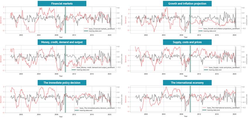
The image above shows what we have done so far. In this part, I am going to create two sentiments:
- Interest rate sentiment based on both BOE Minutes and Speech
- Topical sentiment index based on Minutes only by taking advantage of 6 clear topics in each minute
3.4.1 BOE Interest Rate Sentiment
By applying Region-specific Sentiment Algorithm from the earlier chapter on the cleaned minutes and
speech directly, now we could directly create a monthly dictionary-based interest rate sentiment. To compare
the performance across different types of documents, here I created sentiments based on only minutes, only
speech and both minutes and speech. The performance is measured on full period (1997-2020) and out-of-
sample period (2010-2020). The chart below shows the dictionary created and sentiment performance. The full
dictionary can be viewed at the appendix Figure A.3.
Figure 3.11: Self-created dictionary word cloud. Left are positive sentiment words, right is negative sentiment
Figure 3.12: Dictionary-based method performance on BOE documents after language filtering
22You can also read