Integrating Microsimulation Models of Tax Policy into a DGE Macroeconomic Model: A Canonical Example - imfs-frankfurt.de
←
→
Page content transcription
If your browser does not render page correctly, please read the page content below

Integrating Microsimulation Models of Tax Policy
         into a DGE Macroeconomic Model:
                A Canonical Example ∗
      Jason DeBacker†              Richard W. Evans‡               Kerk L. Phillips§

                                        March 2017
                                         (version 17.03.a)

                                          Abstract
         This paper integrates individual effective tax rates and marginal tax rates
      computed from a microsimulation (partial equilibrium) model of tax policy
      with a dynamic general equilibrium (DGE) model of tax policy that can pro-
      vide macroeconomic analysis or dynamic scores of tax reforms. Our approach
      captures the rich heterogeneity, realistic demographics, and tax-code detail of
      the microsimulation model and allows this detail to inform a general equilibrium
      model with a relatively high degree of heterogeneity. In addition, we propose a
      functional form in which tax rates depend jointly on the levels of both capital
      income and labor income.

      JEL classification: D91, E21, H30

  ∗
     This research benefited from support from the Open Source Policy Center at the Amer-
ican Enterprise Institute as well as from the Becker Friedman Institute at the University of
Chicago. All Python code and documentation for the computational model is available at
https://github.com/rickecon/TaxFuncIntegr, with ongoing development of the model beyond this
paper at https://github.com/open-source-economics/OG-USA.
   †
     Darla Moore School of Business, University of South Carolina, Department of Economics, DMSB
427B, Columbia, SC 29208, (803) 777-1649, jason.debacker@moore.sc.edu.
   ‡
     University of Chicago, Becker Friedman Institute, Saieh Hall, Room 250, Chicago, IL 60637,
(773) 702-9169, rwevans@uchicago.edu.
   §
     Brigham Young University, Department of Economics, 166 FOB, Provo, Utah 84602, (801)
422-5928, kerk phillips@byu.edu.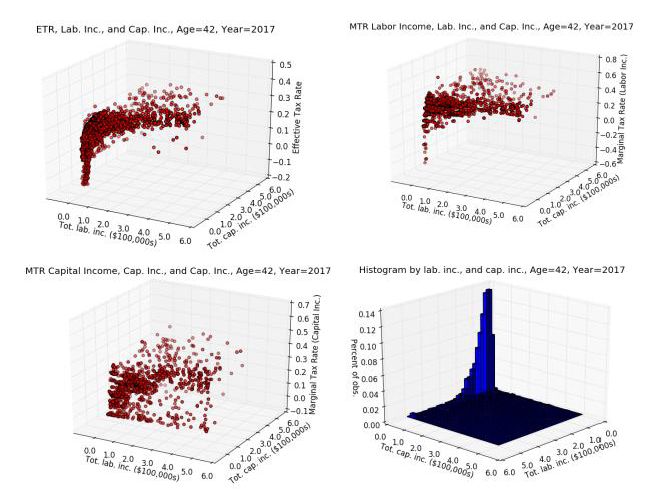
1     Introduction
Heterogeneous agent models have become the norm in macroeconomics. This devel-
opment has added more richness and realism to macroeconomic models and allowed
for the exploration of topics related to distributional issues that could not be oth-
erwise addressed. However, there often remains a lack of detail in the way policy
instruments are incorporated into dynamic general equilibrium models. The gap be-
tween the rich heterogeneity in model agents and lack of policy detail can be especially
striking in the context of models used to evaluate tax policy. This gap is often due
to the intractability of modeling the fine details of real-world policy.
    Krueger and Ludwig (2016) ask policy relevant questions regarding tax policy
and have a rich model comprised of agents with heterogeneous skill-levels, assets, and
age. But they model the tax code using linear tax functions. Even models at the
frontier of the dynamic of analysis of fiscal policy, such as Nishiyama (2015), impose
tax functions that are progressive but do not allow for marginal rates on a particular
income source to be a function of other income.
    Our contributions in this paper are primarily methodological. First, we propose a
flexible functional form for tax rates that has the smoothness and monotonicity prop-
erties necessary for solving a DGE model while retaining much of the heterogeneity
found in microsimulation model tax data. The tax functions that we propose can
capture progressive rates and account for the influence of income across sources on
marginal rates. That is, our tax functions are multivariate, like the income tax code
in the U.S. and many other countries, where income from one source affects marginal
rates from other sources of income. Second, we describe a methodology where one
can easily fit these tax functions using the output of a microsimulation model. The
use of a microsimulation model is important in that these models are able to capture
the rich detail of tax policy and how it affects households with different economic
and demographic characteristics. The tax functions we propose then map the results
of the microsimulation model, the computed average and marginal tax rates, into
parameterized functions that can be used in a macroeconomic model. We tailor our

                                           1
functions here to a specific microsimulation model and DGE model, but the method-
ology we propose can be scaled up or down to account for models with more or less
heterogeneity.
   Our approach has two distinct advantages. It allows the DGE model to capture
more detail of tax policy in than previously used methods. It also greatly reduces the
cost to incorporating rich policy detail and counterfactuals into macroeconomic anal-
ysis. The bridge we build between the microsimulation model and the macroeconomic
model essentially automates this process.
   Others have used parameterized tax functions to represent the tax code in general
equilibrium models. Fullerton and Rogers (1993) estimate tax rate functions that
vary by lifetime income group and age, but their marginal and average rates are not
functions of realized income. Zodrow and Diamond (2013) follow a similar methodol-
ogy. Many of these studies use micro data to estimate the tax functions. For example,
Fullerton and Rogers (1993) use the Panel Study for Income Dynamics to estimate
ordinary least squares models that identify the parameters of their tax functions.
Guner et al. (2014) use data from the Statistics of Income (SOI) Public Use File to
calibrate average and marginal tax rate functions for various definitions of household
income, separately for those with different household structures. Other examples of
the estimations of flexible tax functions on labor or household income (in the U.S.
and across other countries) come from Gouveia and Strauss (1994), Guvenen et al.
(2014), and Holter et al. (2014). Nishiyama (2015) uses a version of the Gouveia and
Strauss (1994) tax function, but does not condition tax functions on age nor does he
allow marginal tax rates to be multivariate functions of the agents’ different income
sources. Rather, the marginal tax rate on labor income is only a function of labor
income and the marginal tax rate on capital income is constant. Nishiyama (2015)
uses ordinary least squares to estimate the parameters of his proposed tax functions
from data produced by the Congressional Budget Offices’ microsimulation model.
   Our approach uses the output of a microsimulation model, Tax-Calculator, to
estimate effective and marginal tax rate functions that jointly vary by age, labor
income, and capital income. This study is the first to incorporate this level of detail

                                            2
into the tax functions used in a DGE model. It is also novel in the integration
between the microsimulation and DGE models. Such integration not only allows one
to estimate tax functions for current law policy, but also to estimate the parameters
of tax functions that specify counterfactual tax policies—even those that adjust tax
policy levers that are difficult to model explicitly in a general equilibrium framework.
        In this paper, we apply our methodology by analyzing the macroeconomics effects
of a simple change in tax policy—a 10-percent reduction in all statutory marginal
tax rates on personal income and a doubling of the standard deduction for each
filer type. For the purposes of our simulations, we assume these changes in tax law
are permanent and are instituted on January 1, 2017 with no anticipatory effects.
This policy experiment is a canonical example, used by Arnold et al. (2004) and
Diamond and Moomau (2003) to show the effects of various modeling approaches to
dynamic analysis of tax policy. In our experiment, we add the increase in the standard
deduction to our policy experiment in order to include a change in the tax code that
differentially affects marginal and average tax rates, which further exemplifies the
power of our method of incorporating microsimulation tax data.
        The paper is organized as follows. Section 2 provides a brief overview of how taxes
enter a dynamic general equilibrium model.1 We then describe the functional form for
the tax functions we use and describe how they map to the DGE model in Section 3.
Section 4 then details how the parameters of these tax functions are estimated from
the output of a microsimulation model. In Section 5 we show how our tax functions
compare to others. We present an illustrative example of our methodology in Section
6, using a canonical tax policy reform. Section 7 concludes.

2         Taxes in a DGE Model
To illustrate how tax policy enters a macroeconomic dynamic general equilibrium
model, we use the overlapping generations model of DeBacker et al. (2015). This
model has some theoretical simplifications, such as deterministic lifetime earnings
    1
        More detail on the DGE model is available in the Appendix.

                                                  3
ability profiles and a government budget constraint that is balanced every period. Our
focus here is independent of the particular DGE model. We are demonstrating how
the richness of tax policy can be tractably integrated into any DGE macroeconomic
model. We provide a full description of the model in Appendix A-1, but here we
focus specifically on the details of the model that are relevant for describing how
and where taxes enter the DGE model. In particular, we describe the dimensions of
heterogeneity in the model and how income taxes affect household decisions.
In DeBacker et al. (2015), agents are heterogeneous in age, their lifetime labor
productivity profiles, and the wealth the model households accumulate (which is
endogenous). In particular, there are seven lifetime income groups in the model.
Income is endogenous, so lifetime income groups are defined by potential earnings and
the earnings profiles we estimate are over hourly earnings.2 The estimated earnings
profiles are shown in Figure 1.
Figure 1: Exogenous life cycle income ability
paths log(ej,s ) with S = 80 and J = 7
Model agents are economically active for as many as S years, facing mortality
risk that is a function of their age, s. Lifetime income groups are noted with the
subscript j and the effective labor units (productivity) over the lifecycle for each type
2
Our methodology to define and estimate these earnings profiles follows Fullerton and Rogers
(1993) and is described in detail in DeBacker et al. (2015).
4is given by ej,s . The model year is denoted by the subscript t. Model agents choose
consumption, ĉj,s,t , savings, b̂j,s,t , and labor supply, n̂j,s,t . The hats over the variables
denote that they have been stationarized (see Appendix A-1 for more details).
Our focus is on individual income taxes. The effect of such taxes on model agents’
decisions is captured in three equations. First, the total income tax paid by the model
agent determines after-tax resources available for consumption and savings. This is
related through the budget constraint, shown in Equation 1:
ˆ j,t
BQ
ĉj,s,t = (1 + rt ) b̂j,s,t + ŵt ej,s nj,s,t + I
− egy b̂j,s+1,t+1 − T̂s,t + T̂tH (1)
λj
where rt is the real interest rate at time t and ŵt is the stationarized wage rate at time
t. The parameter λj is the fraction of the total working households of type j in period
t and term BQj,t represents total bequests from households in income group j who
died at the end of period t − 1. The growth rate in labor augmenting technological
I
change is given by gy . T̂s,t is a function representing income and payroll taxes paid,
which we specify more fully below in equation (2). T̂tH is a lump sum transfer given
to all households, which does not vary with household tax liabilities.3
I
The income tax liability function Ts,t is represented by an effective (i.e., average)
tax rate function times income. Let x ≡ ŵt ej,s nj,s,t represent stationary labor income,
and let y ≡ rt b̂j,s,t represent stationary capital income. Income tax liability is given
as:
I
Ts,t (x, y) = τs,t (x, y) x + y (2)
I
Note that the both the tax liability function Ts,t (x, y) and the effective tax rate
function τs,t (x, y) are functions of stationarized labor income, x, and capital income,
3
In principle, one could specify the government transfer function in much the same way we specify
the tax function. However, given how benefits are administered in the U.S. (in particular, how
benefits schedules vary from state to state), it is difficult to construct a calculator that determines
benefits receipt for individuals under different policy options. This is something we hope to address
in future research, but that is beyond the scope of this paper’s focus on tax policy.
5y, jointly. We detail the parametric specification of the effective tax rate functions
ET Rs,t (x, y) ≡ τs,t (x, y) in Section 3.
The effects of marginal tax rates effects on consumption, savings, and labor supply
can be seen in the necessary conditions characterizing the agent’s optimal choices of
labor supply and savings. The first order condition for the choice of labor is given by:
I
! υ−1 " υ # 1−υ
υ
∂ T̂s,t
n b nj,s,t nj,s,t
(ĉj,s,t )−σ ŵt ej,s − = χs 1−
∂nj,s,t ˜l ˜l ˜l
(3)
∀j, t, and E + 1 ≤ s ≤ E + S
where b̂j,E+1,t = 0 ∀j, t
The left hand side of the equation gives the marginal benefits to additional labor
supply while the right hand side relates the marginal costs from the disutility of
labor supply. The parameter σ is the coefficient of relative risk aversion from the
constant relative risk aversion utility function. χns are age-dependent utility weights
on the disutility of labor supply, ˜l is the maximum hours an agent can work, and the
parameters b and υ are parameters of the disutility of labor function.4
I
∂ T̂s,t
Taxes affect the labor-leisure decision in (3) through the partial derivative, ∂nj,s,t
,
or the change in tax liability from a change in labor supply. We can decompose this
marginal effect in the following way:
I I
∂ T̂s,t ∂ T̂s,t ∂ ŵt ej,s nj,s,t
=
∂nj,s,t ∂ ŵt ej,s nj,s,t ∂nj,s,t
(4)
I
∂ T̂s,t
= ŵt ej,s
∂ ŵt ej,s nj,s,t
Let x ≡ ŵt ej,s nj,s,t and y ≡ rt b̂j,s,t , we define the function describing the marginal tax
I
∂ T̂s,t
rate on labor income as M T Rxs,t (x, y) ≡ ∂x
.
The first order condition for the optimal lifetime savings decisions of an agent are
4
Evans and Phillips (2016) detail how an elliptical functional form can closely approximate the
marginal utilities of the more common constant Frisch elasticity disutility of labor function while
also providing Inada conditions at both the upper and lower bounds of labor supply.
6given by the following dynamic Euler equation:
(ĉj,s,t )−σ = ...
" #!
I
−σ ∂ T̂s+1,t+1
e−gy σ ρs χbj b̂j,s+1,t+1 + β(1 − ρs )(ĉj,s+1,t+1 )−σ 1 + rt+1 − (5)
∂ b̂j,s+1,t+1
∀j, t, and E + 1 ≤ s ≤ E + S − 1
This condition states that, at an optimum, the marginal utility of consumption must
be equation to the benefits from saving. These benefits on the right hand side of
Equation (5) are given by the utility from accidental bequests and the discounted
expected value of future consumption. The parameter χbj is the utility weight on
bequests and ρs is the age-dependent mortality rate. The parameter β reflects the
agents’ rate of time preference.
I
∂ T̂s+1,t+1
Taxes affect savings through the partial ∂ b̂j,s+1,t+1
, which reflects the additional
taxes paid as a function of an additional dollar of savings. As we did with the change
in taxes for a change in labor supply, we can decompose this as:
I
∂ T̂s+1,t+1 ∂ T̂s+1,t+1 ∂r̂t b̂j,s+1,t+1
=
∂ b̂j,s+1,t+1 ∂rt b̂j,s+1,t+1 ∂ b̂j,s+1,t+1
(6)
I
∂ T̂s,t
= rt
∂rt b̂j,s+1,t+1
Let x ≡ ŵt ej,s nj,s,t and y ≡ rt b̂j,s,t , we define the function describing the marginal tax
I
∂ T̂s,t
rate on capital income as M T Rys,t (x, y) ≡ ∂y
.
Any DGE model that incorporates individual income taxes will have some ana-
logue to ET Rs,t (x, y), M T Rxs,t (x, y), and M T Rys,t (x, y). These tax concepts, aver-
age and marginal rates, will enter the model in the same general way as we describe
above. It is these functions that we are estimating directly from microsimulation tax
data. They will vary by age s and time period t and will each be functions of both
labor income x and capital income y. One of the contributions of this paper is the
use of tax rate functions that vary with both labor and capital income. As will be
shown in the next section, this characteristic seems to be an important feature of the
7tax data. With these definitions of the effective and marginal tax rate functions, we
now turn to our parameterized functional form.
3 Tax Functions
Figure 2 shows scatter plots of effective tax rates (ETR), marginal tax rates on labor
income (MTRx), marginal tax rates on capital income (MTRy), and a histogram of
the data points from the Tax-Calculator microsimulation model, each plotted as a
function of labor income and capital income for all 42-year-olds in the year 2017. The
data we use in the Tax-Calculator come from the 2009 IRS Public Use File and a
statistical match of the Current Population Survey (CPS) demographic data.5 Labor
and capital income are truncated at $600,000 in order to more clearly see the shape
of the data in spite of the long right tail of the income distribution. Although there is
noise in the data, effective tax rates are generally increasing in both labor and capital
income at a decreasing rate from some slightly negative level to an asymptote around
30 percent. This regular shape in effective tax rates is observed for all ages in all
years of the budget window, 2017-2026.
Because of the regularity in the shape of the effective tax rates, we choose to fit
a smooth functional form to these data that is able to parsimoniously fit this shape
while also being flexible enough to adjust to a wide range of tax policy changes. Our
functional form, shown in (7) for the effective tax rate, is a Cobb-Douglas aggregator
of two ratios of polynomials in labor and capital income. We use the same functional
form for the effective and marginal tax rate functions. Important properties of this
functional form are that it produces this bivariate negative exponential shape, is
monotonically increasing in both labor income and capital income, and that it allows
for negative tax rates. In order to capture variation in taxes by filer age and model
year, we estimate functions for each model age and every year of the budget-window
that the microsimulation model captures. In this way, we are able to map more of the
5
We discuss this microsimulation model and the data further in Section 4.
8Figure 2: Scatter plot of ETR, MTRx, MTRy, and histogram as functions
of labor income and capital income from microsimulation model:
t = 2017 and s = 42 under current law
∗ Note: Axes in the histogram in the lower-right panel have been switched relative to the other three figures in order
to see the distribution more clearly.
9heterogeneity from the microsimulation into the macro model than can be explicitly
incorporated into a DGE model.
As an example, filing status is correlated with age and income. Thus, although
the DGE model we use does not explicitly account for filing status, we are able to
capture some of the effects of filing status on tax rates by having age and income
dependent functions for effective and marginal tax rates. As another example, in-
vestment portfolio decisions differ over the lifecycle and these are difficult to model
in detail in a DGE model. By using age-dependent tax functions, we are able to
capture some of the differentials in tax treatment across different assets (e.g. rates
on dividends versus capital gains, tax-preferred retirement savings accounts, certain
exemptions for interest income) even if the DGE model does not explicitly model
these portfolio decisions.
Finally, consider that many macroeconomic models assume a single composite
consumption good. Some of this composite good affects tax liability, such as the con-
sumption of charitable contributions or housing. To the extent that the fraction of the
composite good that comes from such consumption varies over a household’s income
and age, these tax functions will capture that, since they are fitted using microeco-
nomic data that includes information on these tax-relevant forms of consumption.
Let x be total labor income, x ≡ ŵt ej,s nj,s,t , and let y be total capital income,
y ≡ rt b̂j,s,t . We then write our tax rate functions as follows.
h iφ h i1−φ
τ (x, y) = τ (x) + shif tx τ (y) + shif ty + shif t
Ax2 + Bx
where τ (x) ≡ (maxx − minx ) + minx
Ax2 + Bx + 1
Cy 2 + Dy
and τ (y) ≡ (maxy − miny ) + miny (7)
Cy 2 + Dy + 1
where A, B, C, D, maxx , maxy , shif tx , shif ty > 0 and φ ∈ [0, 1]
and maxx > minx and maxy > miny
Note that we let τ (x, y) represent the effective and marginal rate functions, ET R(x, y),
M T Rx(x, y) and M T Ry(x, y). We assume the same functional form for each of these
10functions. The parameters values will, in general, differ across the different functions
(effective and marginal rate functions) and by age, s, and tax year, t. We drop the
subscripts for age and year from the above exposition for clarity.
By assuming each tax function takes the same form, we are breaking the analytical
link between the the effective tax rate function and the marginal rate functions. In
particular, one could assume an effective tax rate function and then use the analytical
derivative of that to find the marginal tax rate function. However, we’ve found it
useful to separately estimate the marginal and average rate functions. One reason
is that we want the tax functions to be able to capture policy changes that have
differential effects on marginal and average rates. For example, and relevant to the
policy experiment we present below, a change in the standard deduction for tax payers
would have a direct effect on their average tax rates. But it will have secondary effect
on marginal rates as well, as some filers will find themselves in different tax brackets
after the policy change. These are smaller and second order effects. When tax
functions are are fit to the new policy, in this case a lower standard deduction, we
want them to be able to represent this differential impact on the marginal and average
tax rates. The second reason is related to the first. As the additional flexibility allows
us to model specific aspects of tax policy more closely, it also allows us to better fit
the parameterized tax functions to the data.
The key building blocks of the functional form Equation (7) are the τ (x) and
Ax2 +Bx
τ (y) univariate functions. The ratio of polynomials in the τ (x) function Ax2 +Bx+1
with positive coefficients A, B > 0 and positive support for labor income x > 0
creates a negative-exponential-shaped function that is bounded between 0 and 1, and
the curvature is governed by the ratio of quadratic polynomials. The multiplicative
scalar term (maxx −minx ) on the ratio of polynomials and the addition of minx at the
end of τ (x) expands the range of the univariate negative-exponential-shaped function
to τ (x) ∈ [minx , maxx ]. The τ (y) function is an analogous univariate negative-
exponential-shaped function in capital income y, such that τ (y) ∈ [miny , maxy ].
The respective shif tx and shif ty parameters in Equation (7) are analogous to the
additive constants in a Stone-Geary utility function. These constants ensure that the
11two sums τ (x) + shif tx and τ (y) + shif ty are both strictly positive. They allow for
negative tax rates in the τ (·) functions despite the requirement that the arguments
inside the brackets be strictly positive. The general shif t parameter outside of the
Cobb-Douglas brackets can then shift the tax rate function so that it can accommo-
date negative tax rates. The Cobb-Douglas share parameter φ ∈ [0, 1] controls the
shape of the function between the two univariate functions τ (x) and τ (y).
This functional form for tax rates delivers flexible parametric functions that can
fit the tax rate data shown in Figure 2 as well as a wide variety of policy reforms.
Further, these functional forms are monotonically increasing in both labor income x
and capital income y. This characteristic of monotonicity in x and y is essential for
guaranteeing convex budget sets and thus uniqueness of solutions to the household
Euler equations. The assumption of monotonicity does not appear to be a strong one
when viewing the the tax rate data shown in Figure 2. While it does limit the potential
tax systems to which one could apply our methodology, tax policies that do not satisfy
this assumption would result in non-convex budget sets and thus require non-standard
DGE model solutions methods and would not guarantee a unique equilibrium. The
12 parameters of our tax rate functional form from (7) are summarized in Table 1.
Table 1: Description of tax rate function τ (x, y) parameters
Symbol Description
A Coefficient on squared labor income term x2 in τ (x)
B Coefficient on labor income term x in τ (x)
C Coefficient on squared capital income term y 2 in τ (y)
D Coefficient on capital income term y in τ (y)
maxx Maximum tax rate on labor income x given y = 0
minx Minimum tax rate on labor income x given y = 0
maxy Maximum tax rate on capital income y given x = 0
miny Minimum tax rate on capital income y given x = 0
shif tx shifter > |minx | ensures that τ (x) + shif tx > 0 despite potentially
negative values for τ (x)
shif ty shifter > |miny | ensures that τ (y) + shif ty > 0 despite potentially
negative values for τ (y)
shif t shifter (can be negative) allows for support of τ (x, y) to include
negative tax rates
φ Cobb-Douglas share parameter between 0 and 1
12Figure 3 shows the estimated function surfaces for tax rate functions for the effec-
tive tax rate (ETR), marginal tax rate on labor income (MTRx), and marginal tax
rate on capital income (MTRy) data shown in Figure 2 for age s = 42 individuals
in period t = 2017 under the current law. Section 4.3 details the nonlinear weighted
least squares estimation method of the 12 parameters in Table 1, but before we detail
those methods we show here that the functional form is able to fit the data closely.
And the estimated parameters and the corresponding function surface change when-
ever any of the many policy levers in the microsimulation model that generate the
tax rate data are adjusted. The total tax liability function is simply the effective tax
rate function times total income τ (x, y)(x + y).
I
Ts,t (x, y) ≡ ET Rs,t (x, y) x + y
(8)
h iφ h i1−φs,t
= τs,t (x) + shif tx,s,t τs,t (y) + shif ty,s,t + shif ts,t x + y
s,t
As we describe above, each rate function (ET R, M T Rx, M T Ry) varies by age,
s, and tax year t. This means a large number of parameters must be estimated. In
particular, using our illustrative example with the model of DeBacker et al. (2015), we
will need to fit 12 parameters for each of three tax rate functions for each age (21 to
100) during each of the 10 years of the budget window with the estimated functions in
the last year of the budget window assumed to be permanent. The microsimulation
model we use, Tax-Calculator is able to provide marginal and average tax rates
for 10-years forward from the present.6 The DGE model is solved from the current
period forward through the steady-state. The steady-state is generally arrived at well
beyond a time horizon of 10 years. Thus we allow variation the in the rate functions
only over this 10-year budget window and fix the parameters of the rate functions to
the last year of the window for years t ≥ 10. Thus, in our illustrative example, there
are 2,400 tax rate functions comprised of 28,800 parameters.
6
This is the standard timeframe considered by policy analysts analyzing the effects of tax policy
on the federal budget.
13Figure 3: Estimated tax rate functions of ETR, MTRx, MTRy, and his-
togram as functions of labor income and capital income from
microsimulation model: t = 2017 and s = 42 under current law
∗ Note: Axes in the histogram in the lower-right panel have been switched relative to the other three figures in order
to see the distribution.
14Because we allow these many functions of labor income and capital income to be
independently estimated for each tax rate type, age, and year, we can capture many
of the characteristics and discrete variation in the tax code while still preserving
the smoothness and monotonicity of the tax functions within each type, age, and
year. This monotonicity and smoothness is sufficient to guarantee uniqueness and
tractability of the computational solution of the household Euler equations. Allowing
for different tax rate functions by age and time period also implicitly incorporates
heterogeneity in the data in dimensions that we cannot model in the DGE model,
such as broader income items, deductions items, credits, and filing unit structure. The
effect of such heterogeneity on tax burdens will affect the effective tax rate functions
we fit to the output of the microsimulation model.
Table 2: Average values of φ for ETR,
MTRx, and MTRy for age bins
in period t = 2017
Age ranges
21 to 54 55 to 65 66 to 80 All years
ET R 0.66 0.28 0.38 0.44
M T Rx 0.89 0.31 0.23 0.48
M T Ry 0.77 0.25 0.14 0.43
* Note: Even though agents in the OG model live until age
100, the tax data was too sparse to estimate functions for
ages greater than 80. For ages 81 to 100, we simply assumed
the age 80 estimated tax functional forms.
It is difficult to show all the estimated tax functions for every age and period in
the budget window. But Table 2 gives a description of the estimated values of the
φ parameter. This parameter φ in the tax function (7) governs how important the
interaction is between labor income and capital income for determining tax rates.
The further interior is φ (away from 0 or 1), the more important it is to model tax
rates as functions of both labor income and capital income. And the closer φ is to 1,
the more important is labor income for determining tax rates.
Two key results jump out from Table 2. First, it is clear that the interaction
between labor income and capital income is significant at all ages for determining
15effective tax rates ET R, marginal tax rates on labor income M T Rx, and marginal
tax rates on capital income M T Rx. The last column of Table 2 shows the average
phi value for all ages in the data to be around 0.45 for all three tax rate types. This
suggests that models that use univariate tax functions of any type of income miss
important information and incentives present in the tax code.
A second result from Table 2 is that the relative importance of labor income in
determining tax rates varies over the life cycle in similar ways for each tax rate type
(ET R, M T Rx, and M T Ry). The first three columns of each row of Table 2 show
that labor income is most important for determining tax rates between the ages of 21
and 54 and that capital income is most important for determining tax rates between
the ages of 55 and 65. For marginal tax rates capital income continues to be the most
important determinant after age 65, but capital income and labor income are equally
important determinants of the effective tax rate ET R after age 65. This suggests that
models that use tax functions that do not vary with age also miss some important
information and incentives present in the tax code.
4 Integration of microsimulation model with DGE
model
An important part of the methodology we propose is our integration of tax functions
estimated from the output of a microsimulation model into a DGE model. The nature
of DGE models is such that they cannot accommodate the degree of policy detail and
filer heterogeneity that exist in the microdata. The analytics would be intractable
and the computational burden too high. In addition, finding optimal solutions to the
lifetime problem of each household would be extremely difficult due to the nonconvex
optimization problem created by the kinks and cliffs in the current tax code or in the
proposed policies.
In contrast, microsimulation models are perfectly suited to calculate the total taxes
paid, effective tax rates, and marginal tax rates for a population with richly defined
16demographic heterogeneity. Microsimulation models of tax policy also incorporate
most of the detail in the tax code with respect to specific policy levers. We fit smooth
tax functions with the requisite properties to the tax rates determined through a
microsimulation model. We then use those estimated parametric functions in a DGE
macroeconomic model. In this way, we incorporate complexities of the actual tax code
and their interactions with filer heterogeneity into a macroeconomic model, which is
necessarily limited in terms of how much policy detail and household heterogeneity
can be explicitly represented.
4.1 Microsimulation model: Tax-Calculator
The microsimulation model we use is called Tax-Calculator and is maintained a
group of economists, software developers, and policy analysts.7 Other than being
completely open source, the Tax-Calculator is very similar to other tax calculators
such as NBER’s TaxSim and proprietary models used by think tanks and govern-
mental organizations. For this reason, much of what we say below generalizes if
one were to use those other microsimulation models. In this section, we outline the
main structure of the Tax-Calculator microsimulation model, but encourage the
interested reader to follow the links for more detailed documentation.
Tax-Calculator uses microdata on a sample of tax filers from the tax year 2009
Public Use File (PUF) produced by the IRS.8 These data contain detailed records
from the tax returns of about 200,000 tax filers who were selected from the population
of filers through a stratified random sample of tax returns. These data come from
IRS Form 1040 and a set of the associated forms and schedules. The PUF data are
then matched to the Current Population Survey (CPS) to get imputed values for filer
demographics such as age, which are not included in the PUF, and to incorporate
7
The documentation for using Tax-Calculator is available at
http://taxcalc.readthedocs.org/en/latest/index.html A simple web application that provides
an accessible user interface for Tax-Calculator is available from the Open Source Policy Center
(OSPC) at http://www.ospc.org/taxbrain/. All the source code for the Tax-Calculator is freely
available at https://github.com/open-source-economics/Tax-Calculator.
8
Technically, the Tax-Calculator could use other microdata as a source, but we choose to use
the PUF for the relatively large sample size and the degree of detail provided for various income
and deduction items.
17households from the population of non-filers. The PUF-CPS match includes 219,815
filers.
Since these data are for calendar year 2009, they must be “aged” to be represen-
tative of the potential tax paying population in the years of interest (e.g. the current
year through the end of the budget window). To do this, macroeconomic forecasts
of wages, interest rates, GDP, and other variables are used to grow the 2009 values
to be representative of the values one might see in subsequent years. Adjustments to
the weights applied to each observation in the microdata are also made. More specifi-
cally, weights are adjusted to hit a number of targets in an optimization problem that
sets out to minimize the distance between the extrapolated microdata values and
the targets, with a penalty being applied for large changes in the weight individual
observations from one year to the next. The targets are comprised of a number of
aggregate totals of line items from Form 1040 (and related Schedules) produced by
SOI for the years 2010-2013.9
Using these microdata, Tax-Calculator is able to determine total tax liability
and marginal tax rates by computing the tax reporting that minimizes each filer’s
total tax liability given the filer’s income and deductions items and the parameters
describing tax law. The determination of total tax liability from the microsimulation
model includes federal income taxes and payroll taxes but currently excludes state
income taxes and estate taxes. The output of the microsimulation model includes
forecasts of the total tax liability in each year, marginal tax rates in income sources,
and items from the filers’ tax returns for each of the 219,815 filers in the microdata. To
calculate marginal tax rates on any given income source, the model adds one cent to
the income source for each filing unit in the microdata and then computes the change
in tax liability. The change in tax liability divided by the change in income (one cent)
yields the marginal tax rate. Population sampling weights are determined through
the extrapolation and targeting of the microsimulation model. These weights allow
one to calculate population representative results from the model. One can determine
9
For details on how these data are extrapolated, please see the Tax Data program and associated
documentation.
18changes in tax liability and marginal tax rates across different tax policy options by
doing the same simulation where the parameters describing the tax policy are updated
to reflect the proposed policy rather than the baseline policy. The baseline policy used
by Tax-Calculator is a current-law baseline.
4.2 Mapping income from micro to macro model
To map the output of the microsimulation model, which is based on income reported
on tax returns, to the DGE model, where income is defined more broadly, we use the
following definitions. In computing the effective tax rates from the microsimulation
model, we divided total tax liability by a measure of “adjusted total income”. Ad-
justed total income is defined as total income (Form 1040, line 22) plus tax-exempt in-
terest income, IRA distributions, pension income, and Social Security benefits (Form
1040, lines 8b, 15a, 16a, and 20a, respectively). We consider adjusted total income
from the microsimulation model to be the counterpart of total income in the DGE
model. Total income in the DGE model is the sum of capital and labor income.
We define labor income as earned income, which is the sum of wages and salaries
(Form 1040, line 7) and self-employment income (Form 1040 lines 12 and 18) from
the microdata. Capital income is defined as a residual.10
To get the marginal tax rate on composite income amounts (e.g., labor income
that is the sum of wage and self-employment income), we take a weighted average that
accounts for negative income amounts. In particular, to we calculate the weighted
average marginal tax rate on composite of n income sources as:
Pn
M T Rn ∗ abs(Incomen )
i=1P
M T Rcomposite = n (9)
i=1 abs(Incomen )
When we look at the raw output from the microsimulation model, we find that
there are several observations with extreme values for their effective tax rate. Since
this is a ratio, such outliers are possible, for example when the denominator, adjusted
10
This is not an ideal definition of capital income, since it includes transfers between filers (e.g.,
alimony payments) and from the government (e.g., unemployment insurance), but we have chosen
this definition in order to ensure that all of total income is classified as either capital or labor income.
19total income, is very small. We omit such outliers by making the following restrictions
on the raw output of the microsimulation model. First, we exclude observations with
an effective tax rate greater than 1.5 times the highest statutory marginal tax rate.
Second, we exclude observations where the effective tax rate is less than the lowest
statutory marginal tax rate on income minus the maximum phase-in rate for the
Earned Income Tax Credit (EITC). Third, we drop observations with marginal tax
rates in excess of 99% or below the negative of the highest EITC rate (i.e., -45%
under current law). These exclusions limit the influence of those with extreme values
for their marginal tax rate, which are few and usually result from the income of the
filer being right at a kink in the tax schedule. Finally, since total income cannot be
negative in the DGE model we use, we drop observations from the microsimulation
model where adjusted total income is less than $5.11
Because the tax rates are estimated as functions of income levels in the microdata,
we have to adjust the model income units to match the units of the microdata. To
do this, we find the f actor such that f actor times average steady-state model income
equals the mean income in the final year of the microdata.
XX
f actor ω̄s λj w̄ej,s n̄j,s + r̄b̄j,s = (data avg. income) (10)
s j
To be precise, the income levels in the model, x and y, must be multiplied by this
factor when they are used in the effective tax rate functions, marginal tax rate of
labor income functions, and marginal tax rate of capital income functions of the form
in Equation (7).
4.3 Estimating tax functions
With the output of the microsimulation model cleaned, we move to our estimation.
We estimate a transformation of the ET R, M T Rx, and M T Ry tax rate functions
described in Equation (7) for each age s of the primary filer and time period t in
11
We choose $5 rather than $0 to provided additional assurance that small income values are not
driving large ETRs.
20our data and budget window, respectively (2,400 separate specifications). That is,
∂T ∂T
we estimate τs,t (x, y), ∂x
(x, y)s,t , and ∂y
(x, y)s,t . We transform these functions so
that the labor income, x, and capital income, y, variables in the polynomials are
transformed to percent deviations from their respective means. This helps with the
scale of the variables in the optimization routine. The transformed ETR and MTR
functions are estimated using a constrained, weighted, non-linear least squares esti-
mator. The weighting in this estimator come from the weights assigned to the filers
in the microsimulation model.
Let θs,t = (A, B, C, D, maxx , minx , maxy , miny , shif tx , shif ty , shif t, φ) be the
full vector of 12 parameters of the tax function for a particular age of filers in a
particular year. We first directly specify minx as the minimum tax rate in the data
for age-s and period-t individuals for capital income close to 0 ($0 < y < $3, 000) and
miny as the minimum tax rate for labor income close to 0 ($0 < x < $3, 000). We
then set shif tx = |minx |+ε and shif ty = |miny |+ε so that the respective arguments
in the brackets of (7) are strictly positive. Let θ̄s,t = {minx , miny , shif tx , shif ty } be
the set of parameters we take directly from the data in this way.
We then estimate eight remaining parameters θ̃s,t = (A, B, C, D, maxx , maxy , shif t, φ)
using the following nonlinear weighted least squares criterion,
N h
X i2
θ̂s,t = θ̃s,t : min τi − τs,t xi , yi |θ̃s,t , θ̄s,t wi ,
θ̃s,t
i=1
(11)
subject to A, B, C, D, maxx , maxy > 0,
and maxx ≥ minx , and maxy ≥ miny and φ ∈ [0, 1]
where τi is the effective (or marginal) tax rate for observation i from the microsim-
ulation output, τs,t (xi , yi |θ̃s,t , θ̄s,t ) is the predicted average (or marginal) tax rate for
filing-unit i with xi labor income and yi capital income given parameters θs,t , and wi
is the CPS sampling weight of this observation. The number N is the total number
of observations from the microsimulation output for age s and year t. Figure 3 shows
the typical fit of an estimated tax function τs,t x, y|θ̂s,t to the data. The data in
Figure 3 are the same age s = 42 and year t = 2017 as the data Figure 2.
21The underlying data can limit the number of tax functions that can be estimated.
For example, we use the age of the primary filer from the PUF-CPS match to be
equivalent to the age of the DGE model household. The DGE model we use allows
for individuals up to age 100, however the data contain few primary filers with age
above age 80. Because we cannot reliably estimate tax functions for s > 80, we apply
the tax function estimates for 80 year-olds to those with model ages 81 to 100. In the
case certain ages below age 80 have too few observations to enable precise estimation
of the model parameters, we use a linear interpolation method to find the values for
those ages 21 ≤ s < 80 that cannot be precisely estimated.12
5 A Comparison of Tax Functions
In this section, we provide a comparison of the fit provided by our tax function
specification. We refer the reader to Sections 3 for the description and justification
of of our functional form. We compare our functions to that of Gouveia and Strauss
(1994), which remains one of the more flexible specifications in the literature, and
one of the more widely used functional forms (e.g., see Guvenen et al. (2014) and
Nishiyama (2015)). The Gouveia and Strauss (1994) tax function is given by:
−1
T = ϕ0 [I − (I −ϕ1 + ϕ2 ) ϕ1 ], (12)
where T are total income taxes and I = x + y is total income. We transform this
function to put it in terms of an effective tax rate:
−1
ET R = ϕ0 [I − (I −ϕ1 + ϕ2 ) ϕ1 ]/I. (13)
In addition, we use our microdata from Tax-Calculator to estimate the above
ET R specification separately by tax year and age. This is not done in others’ work
who use the Gouveia and Strauss (1994) functional form, but this will give that
12
We use two criterion to determine whether the function should be interpolated. First, we require
a minimum number of observations of filers of that age and in that tax year. Second, we require
that that sum of squared errors meet a pre-defined threshold.
22specification the best chance to fit the data as closely as our preferred functional
form proposed in this paper. We use the same nonlinear least squares estimator to
estimate the Gouveia and Strauss (1994) functions.
In Figure 4 we compare the Gouveia and Strauss (1994) specification to ours.
In orange, we show our specification when total income is entirely made up of labor
income and in green we show our specification when total income is comprised of 70%
labor income and 30% capital income. The Gouveia and Strauss (1994) specification is
in purple. We can note a number of differences between these specifications from this
picture. First, our specification shows more ability to capture the negative average
tax rates at the lower end of the income distribution. Second, given the ability to
have this negative intercept, our functional form can show more curvature over lower
income ranges, allowing for a better fit to the steep gradient the data show over this
range. Finally, by comparing the orange and green lines, one can see the ability of
the share parameter to account for the role capital income plays in lowering effective
tax rates as total income increases. In particular, our specification allows for the
filers portfolio of income (i.e., the shares of total income derives from labor or capital
income) at affect this average tax rate, which is a novel contribution of our functional
form.
To more precisely test the fit of these specification against each other, Table 3
presents the standard errors of the estimates from these two specifications. The table
shows the over all fit and also splits these out by age. What we find is that the ratio
of polynomials function we propose shows a much better fit to the data, missing the
effective tax rate by just under three percentage points on average, compared to an
error of 5.5 percentage points in the estimated Gouveia and Strauss (1994) model.
23Figure 4: Plot of estimated ET R functions: t =
2017 and s = 42 under current law
Table 3: Standard error of the estimates of ET R functions
for age bins in period t = 2017
Age ranges
All ages 21 to 54 55 to 65 66 to 80
Ratio of polynomials, ET R 2.98 3.42 1.67 2.22
Gouveia and Strauss (1994), ET R 5.50 6.54 2.57 3.11
Note that we compare only the effective tax rate functions since Gouveia and
Strauss (1994) do not separately estimate marginal tax rate functions, as we do.
Instead, they derive the marginal tax rates analytically from their total tax function.
The implication, then, is that the marginal rates derives in this way will not fit the
data as well as the effective tax rates, which were the target of the estimation. As we
note above, we eschewed this approach of analytically deriving the marginal tax rates
in favor of separately estimating the parameters of the effective and marginal tax
rate functions. We’ve found this allows our model to better capture tax policy that
differentially impacts average and marginal rates and to fit the data more closely.
246 A tax experiment
The policy change we consider is a reduction in the statutory marginal rates on
individual filers’ ordinary income and an a doubling of the standard deduction for
each tax filer type. The reduction in marginal rates is the same example used to
illustrate the workings of overlapping generations models by Arnold et al. (2004) and
Diamond and Moomau (2003). To this we add the change in the standard deduction
to show how our methodology can capture policies that change average and marginal
rates in distinct ways. The changes in marginal rates for each bracket are summarized
in Table 4. Table 5 shows the standard deduction by filer type under current law and
under our policy experiment.
Table 4: Statutory marginal tax
rates by bracket under the
baseline current law versus
policy change
Bracket Baseline Policy
1 0.100 0.090
2 0.150 0.135
3 0.250 0.225
4 0.280 0.252
5 0.330 0.297
6 0.350 0.315
7 0.396 0.356
* Note: The income cutoffs for
each of these brackets vary by
filer type.
Using the methodology described above, we use the microsimulation model to
compute effective and marginal tax rates for each filing unit in the microdata under
the baseline and policy tax law. These data are then used in the estimation of the
parameters of tax functions for each tax year, age, and under the baseline and reform
policies. We present the estimated ET R, M T Rx, and M T Ry parametric functions
in Table 6 for age s = 42 period t = 2017 tax filers for both the baseline policy and
the tax experiment. These are only 6 of the 3,600 tax functions that we estimate
25Table 5: Standard deduction by filer
type under the baseline
current law versus policy
change
Filing status Baseline Policy
Single $6,350 $12,700
Married, Filing Jointly $12,700 $25,400
Married, Filing Separately $6,350 $12,700
Head of Household $9,350 $18,700
Widow $12,700 $25,400
Dependent $1,050 $2,100
in the baseline and policy change combined.13 Figure 3 gives a sense of how well
these estimated functions are able to fit the data for our baseline policy. Results are
similar for the reform analyzed, as can be seen from the sum of squared errors from
the non-linear least squares estimates presented in Table 6.
Table 6: Estimated baseline current law and policy change tax
rate function τs,t (x, y) parameters for s = 42, t = 2017
Baseline Policy
Parameter ETR MTRx MTRy ETR MTRx MTRy
A 6.28E-12 3.43E-23 4.32E-11 5.90E-12 3.43E-23 9.49E-11
B 4.36E-05 4.50E-04 5.52E-05 3.61E-05 4.50E-04 2.48E-05
C 1.04E-23 9.81E-12 5.62E-12 1.04E-23 1.13E-11 2.05E-11
D 7.77E-09 5.30E-08 3.09E-06 9.14E-09 1.89E-06 7.08E-06
max x 0.80 0.71 0.44 0.80 0.68 0.80
min x -0.14 -0.17 0.00E+00 -0.14 -0.17 0.00E+00
max y 0.80 0.80 0.13 0.80 0.80 3.83E-03
min y -0.15 -0.42 0.00E+00 -0.15 -0.42 0.00E+00
shif t x 0.15 0.18 4.45E-03 0.15 0.18 0.01
shif t y 0.16 0.43 1.34E-03 0.16 0.43 3.83E-05
shif t -0.15 -0.42 0.00E+00 -0.15 -0.42 0.00E+00
share 0.84 0.96 0.86 0.83 0.96 0.85
Obs. (N) 3,105 3,105 1,990 3,105 3,105 1,990
SSE 9122.68 15041.35 7756.54 8331.02 13921.42 7326.73
13
Three types of tax functions times 10 year in budget window times 60 ages equals 1,800
functions. The rest of the estimated functions are available in two Python pickle files named
TxFuncEst baselineint.pkl and TxFuncEst policyint.pkl in the folder TaxFuncIntegr/Python
of the repository for this paper.
266.1 Static revenue effects
Using the web application for the Tax-Calculator at www.ospc.org/TaxBrain, we
calculate the revenue effects of the proposal to reduce statutory marginal tax rates
by 10 percent for each tax bracket and double the standard deduction for each filer
type. Figure 5 shows a screen shot of the TaxBrain results page, which shows that
the estimated static revenue change is about -$2.4 trillion over 10 years (2017-2026).
Figure 5: Screen shot from Tax-Calculator of static revenue estimate tax
experiment
We use the Tax-Calculator to find the new effective and marginal tax rates faced
by each of the filers represented in the PUF-CPS match under the reform. We use
these data to fit tax functions over income by year and primary filer age. As explained
above, the fitted functions are then used in our DGE model to analyze the effect of
the reform on macroeconomic aggregates and prices.
276.2 Macroeconomic effects
Table 7 displays the percentage changes in aggregate quantities and prices over the
budget window and in the steady state. These are computed through the DGE
model described above, using the estimated tax functions for the baseline and policy
tax parameters. The parameters of the estimated tax functions are given in Table 6.
Table 7: Percent change in macroeconomic variables over the budget
window and in steady-state from policy change
Macroeconomic 2017-
variables 2017 2018 2019 2020 2021 2022 2023 2024 2025 2026 2026 SS
GDP -0.11 0.71 0.71 0.72 0.82 0.83 0.91 0.91 0.86 0.94 0.73 1.44
Consumption 0.44 0.47 0.51 0.57 0.61 0.65 0.69 0.72 0.77 0.79 0.62 1.16
Investment -1.36 1.24 1.16 1.06 1.30 1.22 1.38 1.34 1.08 1.27 0.98 2.09
Hours Worked -0.19 1.13 1.06 1.03 1.14 1.09 1.18 1.14 1.02 1.11 0.97 1.09
Avg. Wage 0.09 -0.42 -0.36 -0.31 -0.32 -0.27 -0.27 -0.23 -0.16 -0.17 -0.24 0.35
Interest Rate -0.30 1.45 1.23 1.07 1.12 0.95 0.96 0.81 0.57 0.63 0.85 -1.33
Total Taxes -1.08 -7.71 -8.99 -9.81 -8.52 -8.65 -8.33 -8.97 -9.14 -8.78 -7.93 -7.08
6.3 Discussion
Qualitatively, the results of the macro model are consistent with economic theory.
The reduction in marginal tax rates increases the incentives to work and save. We
subsequently see increases aggregate hours worked and investment. As a result, both
GDP and consumption increase. The wage and the interest rate tell an interesting
story. Over the budget window, wages are falling and interest rates are increasing
despite aggregate investment increasing by more than aggregate labor. This is a stock
versus flow issue. The initial response to aggregate labor is bigger than that of the
capital stock because it takes time for the capital from investment to accumulate.
However, as the economy approaches the steady-state, the capital accumulation has
caught up to the labor response resulting in a long run increase on the wage and
decrease of interest rates.
Total tax revenues decrease due to the lower tax rates, but the increase in aggre-
gate income that results from the additional investment and labor supply offset the
28revenue losses to some extent. Over the budget window, however, these effects are
modest. Both the static score from TaxBrain (shown in Figure 5) show revenue losses
of about eight percentage points from the reform.
A few caveats about the limitations of the model are in order. Of first order
importance in determining the macroeconomic effects of changes in tax policy are the
assumptions about how such tax changes are financed (see Diamond and Moomau
(2003) for a comparison of results under different financing options). The DGE model
used here has a simple balanced budget requirement for the government. This means
that tax cuts, as we consider here, are financed by immediate reductions in the lump
sum transfers the government makes to all households. The assumption is the most
conducive to reductions in taxes providing positive macroeconomic effects. If these
tax cuts were temporary and financed by future tax increases, the stimulative effects
of such cuts would be substantially reduced. In fact, our long run increase in GDP of
1.4 percent lies well above the upper bounds found by Diamond and Moomau (2003)
and Arnold et al. (2004). Such differences are largely driven by assumptions regarding
how tax cuts are financed, but are also due to differences in model parameterizations
and other features.
Not considered in this model, but also important in determining the macroeco-
nomic effects of fiscal policy, are the policy responses of the central bank. Implicit
in the results presented here is that the central bank does not respond to fiscal pol-
icy. If, for example, the central bank responded by holding interest rates constant,
the supply side effects would be smaller and their would be less of a change in the
macroeconomic aggregates.
Finally, one should note that while the levels of the macroeconomic aggregates
change in the steady state as a result of tax policy, that long run growth rates do
not. These long run growth rates are governed by exogenous changes in population
growth and factor productivity. Thus these long run growth rates, in this framework,
are not dependent on tax policy.
297 Conclusion
Our goal was to introduce a methodology through which researchers and policy an-
alysts could integrate the strengths of a microsimulation model of tax policy into
aggregate models that allow one to understand the macroeconomic impacts of fiscal
policy. We apply this methodology by estimating the the revenue effects of a canonical
example policy change in a microsimulation model and an overlapping generations
DGE model. More broadly, we note that the methodology and underlying source
code for the tax function estimation can be applied to link other microsimulation or
macroeconomic models.
To the extent that a macroeconomic model has more degrees of heterogeneity
than the one used as an example in this paper, one could add further dimensions to
the tax function estimation. Consider a macroeconomic model with heterogeneity in
households to account for differences betweens households with one and two earners.
Assuming the microsimulation model could utilize data that allowed observation of
this household characteristic, one could use the same methods proposed above to esti-
mate tax functions separately for filing units with only a primary filer and those with
primary and secondary filers. Thus these methods can be quite general and utilized
by a wide class of models. The important consideration is the flexible specification
of the tax functions that allow details of tax policy to be mapped to parametric
functions used in macroeconomic models.
A compelling direction of future work integrating microsimulation models with
general equilibrium models lies providing consistency between the macroeconomic
assumptions underlying the microsimulation model and the macroeconomic effects
found in the general equilibrium model. In our use of the Tax-Calculator, and in all
static microsimulation models, it is assumed that macroeconomic variables either re-
main unchanged by policy experiments or a new path for the macroeconomic variables
are produced by reduced form time series models. We could expand our methodology
of integration of the microeconomic and macroeconomic models by providing for the
following iterative procedure: Obtain solutions to the microsimulation model given an
30You can also read