Multivariate Functional Additive Mixed Models
←
→
Page content transcription
If your browser does not render page correctly, please read the page content below
Multivariate Functional Additive Mixed Models
                                               Alexander Volkmann1 , Almond Stöcker1 , Fabian Scheipl2 , and Sonja Greven1
                                               1
                                                   Chair of Statistics, School of Business and Economics, Humboldt-Universität zu Berlin, Germany
                                                           2
                                                             Department of Statistics, Ludwig-Maximilians-Universität München, Germany

                                                                                              Abstract
arXiv:2103.06606v1 [stat.ME] 11 Mar 2021

                                                         Multivariate functional data can be intrinsically multivariate like movement trajectories
                                                     in 2D or complementary like precipitation, temperature, and wind speeds over time at a
                                                     given weather station. We propose a multivariate functional additive mixed model (multi-
                                                     FAMM) and show its application to both data situations using examples from sports science
                                                     (movement trajectories of snooker players) and phonetic science (acoustic signals and ar-
                                                     ticulation of consonants). The approach includes linear and nonlinear covariate effects and
                                                     models the dependency structure between the dimensions of the responses using multivariate
                                                     functional principal component analysis. Multivariate functional random intercepts capture
                                                     both the auto-correlation within a given function and cross-correlations between the mul-
                                                     tivariate functional dimensions. They also allow us to model between-function correlations
                                                     as induced by e.g. repeated measurements or crossed study designs. Modeling the depen-
                                                     dency structure between the dimensions can generate additional insight into the properties
                                                     of the multivariate functional process, improves the estimation of random effects, and yields
                                                     corrected confidence bands for covariate effects. Extensive simulation studies indicate that
                                                     a multivariate modeling approach is more parsimonious than fitting independent univariate
                                                     models to the data while maintaining or improving model fit.

                                                     Keywords: functional additive mixed model; multivariate functional principal components;
                                                     multivariate functional data; snooker trajectories; speech production

                                           1         Introduction
                                           With the technological advances seen in recent years, functional data sets are increasingly multi-
                                           variate. They can be multivariate with respect to the domain of a function, its codomain, or both.
                                           Here, we focus on multivariate functions with a one-dimensional domain f = (f (1) , ..., f (D) ) : I ⊂
                                           R → RD with square-integrable components f (d) ∈ L2 (I), d = 1, ..., D. For this type of data,
                                           we can distinguish two subclasses: One has interpretable separate dimensions and can be seen
                                           as several complementary modes of a common phenomenon (“multimodal” data, cf. Uludağ
                                           and Roebroeck; 2014) as in the analysis of acoustic signals and articulation processes in speech
                                           production in one of our data examples. The codomain then simply is the Cartesian product
                                           S = S (1) × ... × S (D) of interpretable univariate codomains S (d) ⊂ R. The other subclass is
                                           more “intrinsically” multivariate insofar as univariate analyses would not yield meaningful re-
                                           sults. Consider for example two-dimensional movement trajectories as in one of our motivating
                                           applications, where the function measures Cartesian coordinates over time: for fixed trajectories,
                                           rotation or translation of the essentially arbitrary coordinate system would change the results
                                           of univariate analyses. For intrinsically multivariate functional data a multivariate approach
                                           is the natural and preferred mode of analysis, yielding interpretable results on the observation

                                                                                                  1
level. Even for multimodal functional data, a joint analysis may generate additional insight by
incorporating the covariance structure between the dimensions. This motivates the development
of statistical methods for multivariate functional data. We here propose multivariate functional
additive mixed models to model potentially sparsely observed functions with flexible covariate
effects and crossed or nested study designs.
    Multivariate functional data have been the interest in different statistical fields such as clus-
tering (Jacques and Preda; 2014; Park and Ahn; 2017), functional principal component analysis
(Chiou et al.; 2014; Happ and Greven; 2018; Backenroth et al.; 2018; Li et al.; 2020), and regis-
tration (Carroll et al.; 2020; Steyer et al.; 2020). There is also ample literature on multivariate
functional data regression such as graphical models (Zhu et al.; 2016), reduced rank regression
(Liu et al.; 2020), or varying coefficient models (Zhu et al.; 2012; Li et al.; 2017). Yet, so far,
there are only few approaches that can handle multilevel regression when the functional response
is multivariate. In particular, Goldsmith and Kitago (2016) propose a hierarchical Bayesian mul-
tivariate functional regression model that can include subject level and residual random effect
functions to account for correlation between and within functions. They work with bivariate
functional data observed on a regular and dense grid and assume a priori independence between
the different dimensions of the subject-specific random effects. Thus, they model the correlation
between the dimensions only in the residual function. As our approach explicitely models the
dependencies between dimensions for multiple functional random effects and also handles data
observed on sparse and irregular grids on more than two dimensions, the model proposed by
Goldsmith and Kitago (2016) can be seen as a special case of our more general model class.
    Alternatively, Zhu et al. (2017) use a two stage transformation with basis functions for the
multivariate functional mixed model. This allows the estimation of scalar regression models for
the resulting basis coefficients that are argued to be approximately independent. The proposed
model is part of the so called functional mixed model (FMM) framework (Morris; 2017). While
FMMs use basis transformations of functional responses (observed on equal grids) at the start of
the analysis, we propose a multivariate model in the functional additive mixed model (FAMM)
framework, which uses basis representations of all (effect) functions in the model (Scheipl et al.;
2015). The differences between these two functional regression frameworks have been extensively
discussed before (Greven and Scheipl; 2017; Morris; 2017).
    The main advantages of our multivariate regression model, also compared to Goldsmith and
Kitago (2016) and Zhu et al. (2017), are that it is readily available for sparse and irregular
functional data and that it allows to include multiple nested or crossed random processes, both
of which are required in our data examples. The model also directly models the multivariate
covariance structure of all random effects included in the model using functional principal com-
ponents (FPCs). This makes the model representation more parsimonious and allows further
interpretation of the random effect processes, such as their relative importance and their domi-
nating modes. As part of the FAMM framework, our model provides a vast toolkit of modeling
options for covariate and random effects, of estimation and inference (Wood; 2017).
    We illustrate the proposed multivariate functional additive mixed model (multiFAMM) on
two motivating examples. The first (intrinsically multivariate) data stem from a study on the
effect of a training programme for snooker players with a nested study design (shots within
sessions within players) (Enghofer; 2014). The movement trajectories of a player’s elbow, hand,
and shoulder during a snooker shot are recorded on camera, yielding six-dimensional multivariate
functional data (see Figure 1). In the second data example, we analyse multimodal data from
a speech production study with a crossed study design (speakers crossed with words) (Pouplier
and Hoole; 2016) on so-called “assimilation” of consonants. The two measured modes (acoustic
and articulatory, see Figure 3) are expected to be closely related but joint analyses have not yet
incorporated the functional nature of the data.

                                                 2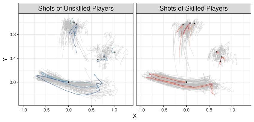
These two examples motivate the development of a regression model for sparse and irreg-
ularly sampled multivariate functional data that can incorporate crossed or nested functional
random effects as required by the study design in addition to flexible covariate effects. The
proposed approach is implemented in R (R Core Team; 2020) in package multifamm. The paper
is structured as follows: Section 2 specifies the multiFAMM and section 3 its estimation process.
Section 4 presents the application of the multiFAMM to the data examples and section 5 shows
the estimation performance of our proposed approach in simulations. Section 6 closes with a
discussion and outlook.

2     Multivariate Functional Additive Mixed Model
2.1     General Model
               (1)          (D)
Let yi (t) = (yi (t), ..., yi (t))> be the multivariate functional response of unit i = 1, ..., N over
t ∈ I, consisting of dimensions d = 1, ..., D. Without loss of generality (w.l.o.g.), we assume
a common one-dimensional interval domain I = [0, 1] for all dimensions, and square-integrable
 (d)
yi ∈ L2 (I). Define L2D (I) := L2 (I) × ... × L2 (I) so that yi ∈ L2D (I). We construct a
multivariate functional mixed model as
                         yi (t) = µ(xi , t) + U (t)zi + it
                                                q
                                                X                                                    (1)
                                = µ(xi , t) +         Uj (t)zij + Ei (t) + it ,   t ∈ I,
                                                j=1

where

                      Uj (t) = (Uj1 (t), ..., UjVUj (t)); j = 1, ..., q,
                             ind.c.
                     Ujv (t) ∼ M GP 0, KUj ; v = 1, ..., VUj ; ∀j = 1, ..., q,
                            ind.c.
                      Ei (t) ∼ M GP (0, KE ) ; i = 1, ..., N, and

                            i.i.d.
                         it ∼ ND 0, Σ̃ = diag(σ12 , ..., σD
                                                           2
                                                             ) ; i = 1, ..., N ;       t ∈ I.
                                                 Pp
We assume an additive predictor µ(xi , ·) = l=1 fl (xi , ·) of fixed effects, which consists of partial
                             (1)             (D)
predictors fl (xi , ·) = (fl (xi , ·), ..., fl (xi , ·))> ∈ L2D (I), l = 1, ..., p, that are multivariate
functions depending on a subset of the vector of scalar covariates xi . This allows to include
linear or smooth covariate effects as well as interaction effects between multiple covariates as in
the univariate FAMM (Scheipl et al.; 2015). Partial predictors may also depend on dimension
specific subsets of covariates.
    For random effects U , we focus on model scenarios with q independent multivariate func-
tional random intercepts for crossed and/or nested designs. For group level v = 1, . . . , VUj within
grouping layer j = 1, . . . , q, these take the value Ujv ∈ L2D (I). For each layer, the Uj1 , ..., UjVUj
present independent copies of a multivariate smooth zero-mean Gaussian random process. Anal-
ogously to scalar linear mixed models, the Ujv model correlations between different response
functions yi within the same group as well as variation across groups. By arranging them in
a (D × VUj ) matrix Uj (t) per t, the jth random intercept can be expressed in the common
mixed model notation in (1) using appropriate group indicators zij = (zij1 , . . . , zijVUj )> for the
respective design.
    Although technically a curve-specific functional random intercept, we distinguish the smooth
residuals Ei ∈ L2D (I) in the notation, as they model correlation within rather than between

                                                          3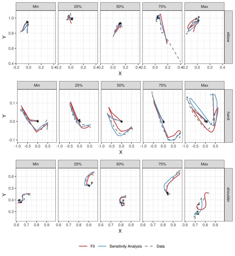
response functions. We write Ev ∈ L2D (I), v = 1, ...,      PVq E with VE = N . The Ei capture smooth
deviations from the group-specific mean µ(xi , ·) + j=1 Uj (·)zij .
 PqFor a more compact representation, we can arrange all Uj (t) and Ei (t) together in a (D ×
( j=1 VUj + N )) matrix U (t) per t, and the group indicators for all layers in a corresponding
              >             >
vector zi = (zi1 , . . . , ziq , e>  >
                                  i ) with ei the i-th unit vector. The resulting model term U (t)zi then
comprises all smooth random functions, accounting for all correlation between/within response
functions yi given the covariates xi as required by the respective experimental design.
   Ei and Ujv are independent copies (ind. c.) of random processes having multivariate  h       D×D co-i
                                                                          (d,e)              (d)   (e)
variance kernels KE , KUj , with univariate covariance surfaces KE (t, t0 ) = Cov Ei (t), Ei (t0 )
                        h                 i
       (d,e)                (d)     (e)
and KUj (t, t0 ) = Cov Ujv (t), Ujv (t0 ) reflecting the covariance between the process dimen-
sions d and e at t and t0 . We call these auto-covariances for d = e and cross-covariance oth-
erwise. The multivariate Gaussian processes are uniquely defined by their multivariate mean
function, here the null function 0, and the multivariate covariance kernels Kg and we write
M GP (0, Kg ) , g ∈ {U1 , . . . , Uq , E}. Note that vectorizing the matrix U (t) allows to formulate
the joint distribution assumption vec(U (t)) ∼ M GP (0, KU ) with KU (t, t0 ) having a block-
diagonal structure repeating each KUj (t, t0 ) for VUj times and KE (t, t0 ) for N times.
    The residual term it reflects additional uncorrelated white noise measurement error, following
a D-dimensional multivariate normal distribution ND with zero-mean and diagonal covariance
matrix Σ̃ = diag(σ12 , ..., σD
                             2
                               ) with dimension specific variances σd2 . To assure model identification
we assume that the different sources of variation Uj (t), j = 1, ..., q, Ei (t), and it are mutually
uncorrelated random processes and that Ei (t) is a residual process with smooth covariance in
contrast to the white noise it .

2.2    FPC Representation of the Random Effects
Model (1) specifies a univariate functional linear mixed model (FLMM) as given in Cederbaum
et al. (2016) for each dimension d. The main difference lies in the multivariate random processes
that introduce dependencies between the dimensions. In order to avoid restrictive assumptions
about the structure of these multivariate covariance operators, which would typically be very
difficult to elicit a priori or verify ex post, we estimate them directly from the data. The
main difficulty then becomes computationally efficient estimation, which is already costly in the
univariate case. Especially for higher dimensional multivariate functional data, accounting for
the cross-covariances can become a complex task, which we tackle with multivariate functional
principal component analysis (MFPCA).
    Given the covariance operators (see Section 3), we represent the multivariate random effects
in model (1) using truncated multivariate Karhunen-Loève (KL) expansions
                                  MUj
                                  X
                      Ujv (t) ≈         ρUj vm ψUj m (t), j = 1, ..., q; v = 1, ..., VUj ,
                                  m=1
                                                                                                         (2)
                                  ME
                                  X
                       Ev (t) ≈         ρEvm ψEm (t), v = 1, ..., N,
                                  m=1

                                                                             (1)      (D)
where the orthonormal multivariate eigenfunctions ψgm = (ψgm , ..., ψgm )> ∈ L2D (I), m =
1, ..., Mg , g ∈ {U1 , ..., Uq , E} of the corresponding covariance operators with truncation lag Mg
are used as basis functions and the random scores ρgvm ∼ N (0, νgm ) are independent and identi-
cally distributed (i.i.d.) with ordered eigenvalues νgm of the corresponding covariance operator.

                                                       4
Note that the assumption of Gaussianity for the random processes can be relaxed. For non-
Gaussian random processes, the KL expansion still gives uncorrelated (but non-normal) scores
and estimation based on a penalized least squares (PLS) criterion (see Section 3.2) remains
reasonable.
    Using KL expansions gives a parsimonious representation of the multivariate random pro-
cesses that is an optimal approximation with respect to the integrated squared error (cf. Ramsay
and Silverman; 2005), as well as interpretable basis functions capturing the most prominent
modes of variation of the respective process. The distinct feature of this approach is that the
multivariate FPCs directly account for the dependency structure of each random process across
the dimensions. If, by contrast, e.g. splines were used in the basis representation of the random
effects, it would be necessary to explicitly model the cross-covariances of each random process
in the model (cf. Li et al.; 2020). Multivariate eigenfunctions, however, are designed to incor-
porate the dependency structure between dimensions and allow the assumption of independent
(univariate) basis coefficients ρgvm via the KL theorem (see e.g. Happ and Greven; 2018). This
leads to a parsimonious multivariate basis for the random effects, where a typically small vector
of scalar scores ρgvm common to all dimensions represents nearly the entire information about
these D-dimensional processes.

3     Estimation
We use a two-step approach to estimate the multiFAMM and the respective multivariate co-
variance operators. In a first step (section 3.1), the D-dimensional eigenfunctions ψgm (t) with
their corresponding eigenvalues νgm are estimated from their univariate counterparts following
Cederbaum et al. (2018) and Happ and Greven (2018). These estimates are then plugged into
(2) and we represent the multiFAMM as part of the general FAMM framework (section 3.2)
by suitable re-arrangement. Consequently, the regression results are conditional on the esti-
mated spectral decompositions. Alternatively, we can view the estimated ψgm (t) simply as an
empirically derived basis that parsimoniously represents the patterns in the observed data.

3.1    Step 1: Estimation of the Eigenfunction Basis
Step 1 (i): Univariate Mean Estimation
In a first step, we obtain preliminary estimates of the dimension specific means µ(d) (xi , t) =
Pp      (d)
  l=1 fl (xil , t) using univariate FAMMs. We model

                              (d)                       (d)
                             yi (t) = µ(d) (xi , t) + it ; d = 1, . . . , D                    (3)
                                                                      (d)
independently for all d with i.i.d. Gaussian random variables it . The estimation of µ(d) (xi , t)
proceeds analogously to the estimation of the multiFAMM described in section 3.2. It is based on
                                                   (d)
the (potentially sparse) evaluation points of the yi (t), whose locations on the interval I can vary
across dimensions. Model (3) thus accommodates sparse and irregular multivariate functional
data and implies a working independence assumption across scalar observations within and across
functions.

Step 1 (ii): Univariate Covariance Estimation
                                                                       (d)     (d)
This preliminary mean function is used to centre the data ỹi (t) = yi (t) − µ̂(d) (xi , t) in
order to detrend them for covariance estimation. Cederbaum et al. (2016) already find that

                                                   5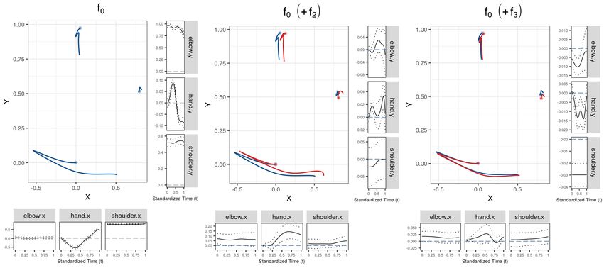
for this purpose, the working independence assumption in (3) gives reasonable results. The
expectation
            of the
                   crossproducts
                           h      of the centred
                                           i     data then coincides with the auto-covariance, i.e.
     (d)   (d) 0             (d)     (d) 0
E ỹi (t)ỹi0 (t ) ≈ Cov yi (t), yi0 (t ) . For the independent random components specified
in model (1), this overall covariance decomposes additively into contributions from each random
process as
                                  Xq
                   (d)    (d)           (d,d)                 (d,d)
               E ỹi (t)ỹi0 (t0 ) ≈   KUj (t, t0 )δvj vj0 + KE (t, t0 ) + σd2 δtt0 δii0 ,

                                                                                                         (4)
                                        j=1

using indicators δxx0 that equal one for x = x0 and zero otherwise. The indicator δvj vj0 thus
identifies if the curves in the crossproduct belong to the same group vj of the jth layer. Using t,
t0 , and the indicators δvj vj0 , δtt0 , δii0 as covariates and the crossproducts of the centred observations
                                                                      (d,d)       (d,d)          (d,d)
as responses, we can estimate the auto-covariances KU1 , ..., KUq , and KE         of the random
processes using symmetric additive covariance smoothing (Cederbaum et al.; 2018). This extends
the univariate approach proposed by Cederbaum et al. (2016). In particular, we also allow a
nested random effects structure as required for the snooker training application in section 4.1
by specifying the indicator of the nested effect as the product of subject and session indicators.
Note that estimating (4) also yields estimates of the dimension specific error variances σd2 as a
byproduct.

Step 1 (iii): Univariate Eigenfunction Estimation
Based on the covariance kernel estimates, we apply separate univariate functional principal com-
ponent analyses (FPCAs) for each random process by conducting an eigendecomposition of the
respective linear integral operator. Practically, each estimated process- and dimension-specific
auto-covariance is re-evaluated on a dense grid so that a univariate FPCA can be conducted.
Eigenfunctions with non-positive eigenvalues are removed to ensure positive definiteness, and
further regularization by truncation based on the proportion of variance explained is possible
(see e.g. Di et al.; 2009; Peng and Paul; 2009; Cederbaum et al.; 2016). However, we suggest to
keep all univariate FPCs with positive eigenvalues for the computation of the MFPCA in order
to preserve all important modes of variation and cross-correlation in the data.

Step 1 (iv): Multivariate Eigenfunction Estimation
The estimated univariate eigenfunctions and scores are then used to conduct an MFPCA for each
of the g multivariate random processes separately. The MFPCA exploits correlations between
univariate FPC scores across dimensions to reduce the number of basis functions needed to
sufficiently represent the random processes. We base the MFPCA on the following definition of
a (weighted) scalar product
                                       D
                                       X          Z
                        hhf , gii :=         wd       f (d) (t)g (d) (t)dt,   f , g ∈ L2D (I),           (5)
                                       d=1        I

for the response space with positive weights wd , d = 1, ..., D and the induced norm denoted by
||| · |||. The corresponding covariance operators Γg : L2D (I) → L2D (I) of the multivariate random
processes Ujv and Ev are then given by (Γg f )(t) = hhf , Kg (t, ·)ii, g ∈ {U1 , ..., Uq , E}. The
standard choice of weights in our applications is w1 = ... = wD = 1 (unweighted scalar product)
but other choices are possible. Consider for example a scenario where dimensions are observed
with different amounts of measurement error. If variation in dimensions with a large proportion

                                                            6
1
of measurement error is to be downweighted, we propose to use wd =          σ̂d2
                                                                                   with the dimension
specific measurement error variance estimates       σ̂d2
                                                   obtained from (4).
    Happ and Greven (2018) show that estimates of the multivariate eigenvalues νgm of Γg can
be obtained from an eigenanalysis of a covariance matrix of the univariate random scores. The
corresponding multivariate eigenfunctions ψgm can be obtained as linear combinations of the
univariate eigenfunctions with the weights given by the resulting eigenvectors. The estimates
ψ̂gm are then substituted for the basis functions of the truncated multivariate KL expansions of
the random effects Ujv and Ev in (2). Note that for each random process g, the maximum number
of FPCs is given by the total number of univariate eigenfunctions included in the estimation
process of the MFPCA of g. To achieve further regularization and analogously to Cederbaum
et al. (2016), we propose to choose truncation lags Mg for each KL expansion of the multivariate
random processes using a prespecified proportion of explained variation.

Step 1 (v): Multivariate Truncation Lag
We offer two different approaches for the choice of truncation lags Mg based on different variance
decompositions (derivation in Appendix A):

                              XD        Z
                                                    (d)
                                                               X MX
                                                                  g =∞       D
                                                                             X
         E |||yi − µ(xi )|||2 =                                                wd σd2 |I|,

                                  wd           Var yi (t) dt =         νgm +                      (6)
                                   d=1     I                     g   m=1       d=1
                           Z
                                      (d)
                                                 X MX
                                                    g =∞
                                                                (d) 2
                                                                   || + σd2 |I|

                     and         Var yi (t) dt =         νgm ||ψgm                                (7)
                             I                       g     m=1

with |I| the length of the interval I (here equal to one) and || · || the L2 norm. Multivariate
variance decomposition (6) uses the (weighted) sum of total variation in the data across dimen-
sions. Using (6), we select the FPCs with highest associated eigenvalues νgm over all random
processes g until their sum reaches a prespecified proportion (e.g. 0.95) of the total variation. For
the approach based on the univariate variance (7), we require Mg to be the smallest truncation
lag for which at least a prespecified proportion of variance is explained on every dimension d.
This second choice of Mg might be preferable in situations where the variation is considerably
different (in amount or structure) across dimensions, whereas the first approach gives a more
parsimonious representation of the random effects. Note that both approaches can lead to a
simplification of the multiFAMM if Mg = 0 is chosen for some g.

3.2    Step 2: Estimation of the multiFAMM
In the following, we discuss estimating the multiFAMM given the estimated multivariate FPCs.
We base the proposed model on the general FAMM framework of Scheipl et al. (2015), which
models functional responses using basis representations. To make the extension of the FAMM
framework to multivariate functional data more apparent, the multivariate response vectors
and the respective model matrices are stacked over dimensions, so that every block has the
structure of a univariate FAMM over all observations i. This gives concatenated basis functions
with discontinuities between the dimensions. The fixed effects are modelled analogously to the
univariate case by interacting all covariate effects with a dimension indicator. The random effects
are based on the parsimonious, concatenated multivariate FPC basis.

                                                     7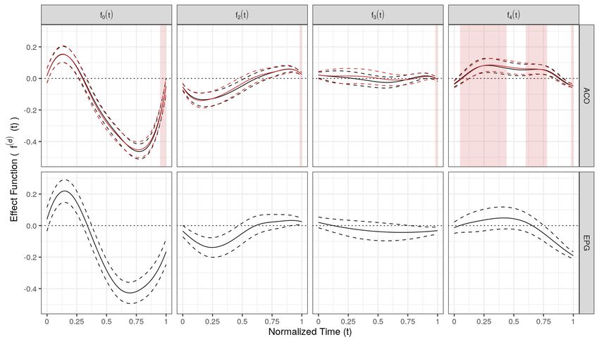
Matrix Representation
For notational simplicity and w.l.o.g. we assume that the functions are observed on a fixed grid
                                                      (d)       (d)                (d)
of time points t = (t(1) , ..., t(D) )> with t(d) = (t1 , ..., tN ) and identical ti ≡ (t1 , ..., tT ) over
all N individuals and D dimensions. However, our framework allows for sparse functional data
using different grids per dimension and per observed function as in the two applications (Section
4). Correspondingly, y = (y (1)> , ..., y (D)> )> is the DN T -vector of stacked observations with
          (d)>      (d)>             (d)    (d)     (d)
y (d) = (y1 , ..., yN )> and yi = (yi1 , ..., yiT )> . Model (1) on this grid can be written as
                                           y = Φθ + Ψρ +                                                  (8)
with Φ, Ψ the model matrices for the fixed and random effects, respectively, θ, ρ the vectors
of coefficients and random effect scores to be estimated, and  = ((1)> , ..., (D)> )> , (d) =
  (d)        (d)        (d)
(11 , ..., 1T , ..., N T )> the vector of measurement errors. We have  ∼ N (0, Σ) with Σ =
diag(σ12 , ..., σD2
                     ) ⊗ IN T , the Kronecker product denoted by ⊗, and the (N T × N T ) identity
matrix IN T .
    We estimate θ and ρ by minimizing the PLS criterion
                                                         p
                                                         X                               X
          (y − Φθ − Ψρ)Σ−1 (y − Φθ − Ψρ)> +                    θl> Pl (λxl , λtl )θl +       λg ρ>
                                                                                                 g Pg ρg   (9)
                                                         l=1                             g

using appropriate penalty matrices Pl (λxl , λtl ) and
                                                    Pg for the fixed effects
                                                                           and random
                                                                                      effects,
                                                      (1)  (D)               (1) (D)
respectively, and smoothing parameters λxl = λxl , ..., λxl , λtl = λtl , ..., λtl , and λg .
The model and penalty matrices as well as the parameter vectors of (8) and (9) are discussed in
detail below.

Modeling of Fixed Effects

The block diagonal matrix Φ = diag Φ(1) , ..., Φ(D) models the fixed effects separately on each
dimension as in a FAMM (Scheipl et al.; 2015). The (DN T × b) matrix Φ consists of the design
                            (d)     (d)                                             (d)
matrices Φ(d) = (Φ1 | ... | Φp ) that are constructed for the p partial predictors fl (x, t(d) ),
                                                                               (d)
which correspond to the N T -vectors of evaluations of the effect functions fl . The vectors
of scalar covariates xi are repeated T times to form the matrix of covariate information x =
(x1 , ..., x1 , ..., xN )> . We use the basis representations
                              (d)              (d) (d)           (d)      (d)   (d)
                            fl (x, t(d) ) ≈ Φl θl        = (Φxl        Φtl )θl ,

where A B denotes the row tensor product (A ⊗ 1>                >
                                                        b ) · (1a ⊗ B) of the (h × a) matrix A and the
(h × b) matrix B with element-wise multiplication · and 1c the c-vector of ones. This modeling
                                   (d)                   (d)                    (d)                 (d)
approach combines the (N T × bxl ) basis matrix Φxl with the (N T × btl ) basis matrix Φtl .
                                                                                   (d)
These matrices contain the evaluations of suitable marginal bases in x and t , respectively. For
                                                  (d)
a linear effect, for example, the basis matrix Φxl is specified as the familiar linear model design
                                 (d)                (d)                                   (d)
matrix x for the linear effect fl (x, t(d) ) = xβl (t(d) ) with coefficient function βl (t(d) ). For
                       (d)           (d)                                (d)
a nonlinear effect fl (x, t(d) ) = gl (x, t(d) ), the basis matrix Φxl contains an (e.g. B-spline)
                                                                                                     (d)
basis representation analogously to a scalar additive model. For the functional intercept, Φxl
                                                                    (d)
is a vector of ones, and we generally use a spline basis for Φtl . For a complete list of possible
effect specifications with examples, we refer to Scheipl et al. (2015). The tensor product basis
                        (d) (d)                                   (d)                         (d)
is weighted by the bxl btl unknown basis coefficients in θl . Stacking the vectors θl gives
          (d)>       (d)>                                                                       (d) (d)
θ (d) = (θ1 , ..., θp )> and finally the b-vector θ = (θ (1)> , ..., θ (D)> )> with b = d l bxl btl .
                                                                                        P   P

                                                    8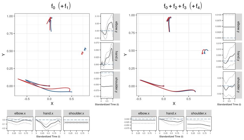
Choosing the number of basis functions is a well known challenge in the estimation of nonlin-
ear or functional effects. We introduce regularization by a corresponding quadratic penalty term
in (9). Let θl contain the coefficients corresponding to the partial predictor l and order it by
dimensions. The penalty Pl (λxl , λtl ) is then constructed from the penalty on the marginal basis
                              (d)
for the covariate effect, Pxl , and the penalty on the marginal basis over the functional index,
  (d)
Ptl . Specifically, Pl (λxl , λtl ) is a block-diagonal matrix with blocks for each d corresponding to
                                                             (d) (d)            (d)         (d)
the Kronecker sums of the marginal penalty matrices λxl Pxl ⊗ Ib(d) + λtl Ib(d) ⊗ Ptl (Wood;
                                                                          tl         xl
2017). A standard choice for these marginal penalty matrices given a B-splines basis representa-
tion are second or third order difference penalties, thus approximately penalizing squared second
or third derivatives of the respective functions (Eilers and Marx; 1996). For unpenalized effects
                                                                      (d)
such as a linear effect of a scalar covariate, the corresponding Pxl is simply a matrix of zeroes.

Modeling of Random Effects
We represent the DN T -vectors Uj (t) = (Uj (t(1) )> , ..., Uj (t(D) )> )> , E(t) = (E(t(1) )> , ..., E(t(D) )> )>
with Uj (t(d) ), E(t(d) ) containing the evaluations of the univariate random effects for the corre-
sponding groups and time points using the basis approximations

              Uj (t) ≈ ΨUj ρUj = (δUj        Ψ̃Uj )ρUj ,   E(t) ≈ ΨE ρE = (δE         Ψ̃E )ρE .

The vth column in the (DN T × Vg ), g ∈ {U1 , ..., Uq , E} indicator matrix δg indicates whether
a given row is from the vth group of the corresponding grouping layer. Thus, the rows of
                                                                                   >
the indicator matrix δg contain repetitions of the group indicators zij              and e>i in model (1).
For the smooth residual, δE simplifies to 1D ⊗ (IN ⊗ 1T ). The (DN T × Mg ) matrix Ψ̃g =
   (1)>      (D)> >                                                                                (d)
(Ψ̃g |...|Ψ̃g    ) comprises the evaluations of the Mg multivariate eigenfunctions ψgm (t) on
                                                                                                          (d)
dimensions d = 1, ..., D for the N T time points contained in the (N T × Mg ) matrix Ψ̃g .
The Mg Vg vector ρg = (ρ>                >
                              g1 , ..., ρgVg )
                                              >
                                                 with ρgv = (ρgv1 , ..., ρgvMg )> stacks all the unknown
                                                                             P
random scores for the functional random effect g. The (DN T × g Mg Vg ) model matrix Ψ =
(ΨU1 |...|ΨUq |ΨE ) then
                      P combines all random >          effect design matrices. Stacking the vectors of
                                                                 >     > >
random scores in a       g M  g V g  vector    ρ =  (ρU1 , ..., ρUq , ρE ) lets us represent all functional
random intercepts in the model via Ψρ.
    For a given functional random effect, the penalty takes the form ρ>                     >
                                                                                 g Pg ρg = ρg (IVg ⊗ P̃g )ρg ,
where IVg corresponds to the assumed independence between the Vg different groups. The diago-
nal matrix P̃g = diag(νg1 , ..., νgMg )−1 contains the (estimated) eigenvalues νgm of the associated
multivariate FPCs. This quadratic penalty is mathematically equivalent to a normal distribu-
tion assumption on the scores ρgv with mean zero and covariance matrix P̃g−1 , as implied by the
KL theorem for Gaussian random processes. Note that the smoothing parameter λg allows for
additional scaling of the covariance of the corresponding random process.

Estimation
We estimate the unknown smoothing parameters in λxl , λtl , and λg using fast restricted max-
imum likelihood (REML)-estimation (Wood; 2017). The standard identifiability constraints of
FAMMs are used (Scheipl et al.; 2015). In particular, in addition to the constraints for the
fixed effects, the multivariate random intercepts are subject to a sum-to-zero constraint over all
evaluation points as given by e.g. Goldsmith et al. (2016).
    We propose a weighted regression approach to handle the heteroscedasticity assumption con-
tained in Σ. We weigh each observation proportionally to the inverse of the estimated univariate

                                                      9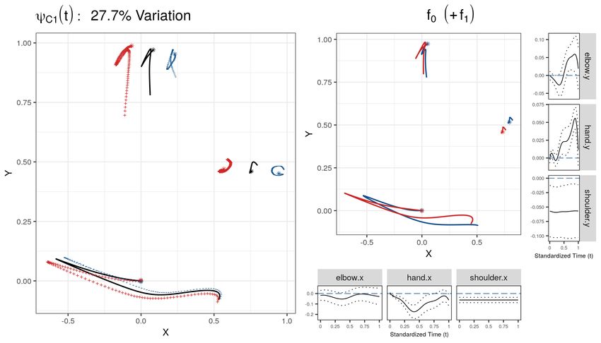
measurement error variances σ̂d2 from the estimation of the univariate covariances (4). Alter-
natively, updated measurement error variances can be obtained from fitting separate univariate
FAMMs on the dimensions using the univariate components of the multivariate FPCs basis. In
practice, we found that the less computationally intensive former option gives reasonable results.
     As our proposed model is part of the FAMM framework, inference for the multiFAMM is read-
ily available based on inference for scalar additive mixed models (Wood; 2017). Note, however,
that all inferential statements are not only conditional on the estimated multivariate eigenfunc-
tion bases but also on the chosen smoothing parameters. The estimation process readily provides
i.a. standard errors for the construction of point-wise univariate confidence bands (CBs).

3.3    Implementation
We provide an implementation of the estimation of the proposed multiFAMM in the multifamm R
package. It is possible to include up to two functional random intercepts in U (t), which can have
a nested or crossed structure, in addition to the curve-specific random intercept Ei (t). While
including e.g. functional covariates is conceptually straightforward (see Scheipl et al.; 2015), our
implementation is restricted to scalar covariates and interactions thereof. We provide different
alternatives for specifying the multivariate scalar product, the multivariate cut-off criterion, and
the covariance matrix of the white noise error term. Note that the estimated univariate error
variances have been proposed as weights for two separate and independent modeling decisions: as
weights in the scalar product of the MFPCA and as regression weights under heteroscedasticity
across dimensions.

4     Applications
We illustrate the proposed multiFAMM for two different data applications corresponding to
intrinsically multivariate and multimodal fuctional data. The presentation focuses on the first
application with a detailed description of the multimodal data application in Appendix C. We
provide the data and the code to produce all analyses in the github repository multifammPaper.

4.1    Snooker Training Data
Data Set and Preprocessing
In a study by Enghofer (2014), 25 recreational snooker players split into two groups, one of
which had instructions to follow a self-administered training schedule over the next six weeks
consisting of exercises aimed at improving snooker specific muscular coordination. The second
was a control group. Before and after the training period, both groups were recorded on high
speed digital camera under similar conditions to investigate the effects of the training on their
snooker shot of maximal force. In each of the two recording sessions, six successful shots per
participant were videotaped. The recordings were then used to manually locate points of interest
(a participant’s shoulder, elbow, and hand) and track them on a two-dimensional grid over the
course of the video. This yields a six dimensional functional observation per snooker shot, i.e. a
two-dimensional movement trajectory for each point of interest (see Figure 1).
   In their starting position (hand centred at the origin), the snooker players are positioned
centrally in front of the snooker table aiming at the cue ball. From their starting position, the
players draw back the cue, then accelerate it forwards and hit the cue ball shortly after their
hands enter the positive range of the horizontal x axis. After the impulse onto the cue ball, the
hand movement continues until it is stopped at a player’s chest. Enghofer (2014) identify two

                                                10
Figure 1: Left: Screenshot of software for tracking (blue lines) the points of interest (circles).
Right: Two-dimensional trajectories of the snooker training data set (grey curves, right). For
both groups of skilled and unskilled participants, three randomly selected observations are high-
lighted. Every colour corresponds to one multivariate observation, i.e. one observation consists
of three trajectories: elbow (top), shoulder (right), hand (bottom). The start of the exemplary
trajectories are marked with a black asterisk with the hand trajectory centred at the origin.
underlying techniques that a player can apply: dynamic and fixed elbow. With a dynamic elbow,
the cue can be moved in an almost straight line (piston stroke) whereas additionally fixing the
elbow results in a pendular motion (pendulum stroke). In both cases, the shoulder serves as a
fixed point and should be positioned close to the snooker table.
We adjust the data for differences in body height and relative speed (Steyer et al.; 2020)
and apply a coarsening method to reduce the number of redundant data points. Appendix B
provides a detailed description of the data preprocessing. As some recordings and evaluations
of bivariate trajectories are missing, the final data set contains 295 functional observations with
a total of 56,910 evaluation points. These multivariate functional data are irregular and sparse,
with a median of 30 evaluation points per functional observation (minimum 8, maximum 80) for
each of the six dimensions.
Model Specification
We estimate the following model
yijh (t) = µ(xij , t) + Bi (t) + Cij (t) + Eijh (t) + ijht , (10)
with i = 1, ..., 25 the index for the snooker player, j = 1, 2 the index for the session, h = 1, ..., Hij
the index for the typically six snooker shot repetitions in a session, and t ∈ [0, 1] relative time.
Correspondingly, Bi (t) is a subject-specific random intercept, Cij (t) is a nested subject-and-
session-specific random intercept, and Eijh (t) is the shot-specific random intercept (smooth
residual). The nested random effect Cij (t) is supposed to capture the variation within players
between sessions (e.g. differences due to players having a good or bad day). Different positioning
of participants with respect to the recording equipment or the snooker table as well as shot to
shot variation are captured by the smooth residual Eijh (t). The white noise measurement error
ijht is assumed to follow a zero-mean multivariate normal distribution with covariance matrix
σ 2 I6 , as all six dimensions are measured with the same set-up. The additive predictor is defined
11as
µ(xij , t) = f0 (t) + skilli · f1 (t) + groupi · f2 (t) + sessionj · f3 (t)
+ groupi · sessionj · f4 (t).
The dummy covariates skilli and groupi indicate whether player i is an advanced snooker
player and belongs to the treatment group (i.e. receives the training programme), respectively.
Note that the snooker players self-select into training and control group to improve compliance
with the training programme, which is why we include a group effect in the model. The dummy
covariate sessionj indicates whether the shot j is recorded after the training period. The effect
function f4 (t) can thus be interpreted as the treatment effect of the training programme.
Cubic P-splines with first order difference penalty, penalizing deviations from constant func-
tions over time, with 8 basis functions are used for all effect functions in the preliminary mean
estimation as well as in the final multiFAMM. For the estimation of the auto-covariances of the
random processes, we use cubic P-splines with first order difference penalty on five marginal basis
functions. We use an unweighted scalar product (5) for the MFPCA to give equal weight to all
spatial dimensions, as we can assume that the measurement error mechanism is similar across
dimensions. Additionally, we find that hand, elbow, and shoulder contribute roughly the same
amount of variation to the data, cf. Table 1 in Appendix B.3, where we also discuss potential
weighting schemes for the MFPCA. The multivariate truncation lag is chosen such that 95% of
the (unweighted) sum of variation (6) is explained.
Results
The MFPCA gives sets of five (for C and E) and six (for B) multivariate FPCs that explain
95% of the total variation. The estimated eigenvalues allow to quantify their relative importance.
Approximately 41% of the total variation (conditional on covariates) can be attributed to the
nested subject-and-session-specific random intercept Cij (t), 33% to the subject-specific random
intercept Bi (t), 14% to the shot-specific Eijh (t), and 7% to white noise. This suggests that day
to day variation within a snooker player is larger than the variation between snooker players.
Note that these proportions are based on estimation step 1 (see Section 3.1).
The left plot of Figure 2 displays the first FPC for C, which explains about 28% of total
variation. A suitable multiple of the FPCs is added (+) to and subtracted (−) from the overall
mean function (black solid line, all covariate values set to 0.5). We find that the dominant mode
of the random subject-and-session specific effect influences the relative positioning of a player’s
elbow, shoulder, and hand. Enghofer (2014) argue from a theoretical point that the ideal starting
position should place elbow and hand in a line perpendicular to the plane of the snooker table
(corresponding to the x axis). The most prominent mode of variation captures deviations from
this ideal starting position found in the overall mean. The next most important FPC ψB1 of the
subject-specific random effect, which explains about 15% of total variation, represents a subject’s
tendency towards the piston or pendulum stroke (see Appendix Figure 8). This additional insight
into the underlying structure of the variance components might be helpful for e.g. developing
personalized training programmes.
The central plot on the right of Figure 2 compares the estimated mean movement trajectory
for advanced snooker players (red) to that in the reference group (blue). It suggests that more
experienced players tend towards the dynamic elbow technique, generating a hand trajectory
resembling a straight line (piston stroke). Uncertainties in the trajectory could be represented
by pointwise ellipses, but inference is more straightforward to obtain from the univariate effect
functions. The marginal plots display the estimated univariate effects with pointwise 95% con-
fidence intervals. Even though we find only little statistical evidence for increased movement of
12Figure 2: Left: Dominant mode (ψC1 ) of the subject-and-session-specific random effect, explain-
ing 27.7% of total variation and shown as mean trajectory (black solid) plus (red +) or minus
√
(blue −) 2 νC1 times the first FPC. An asterisk marks the start of a trajectory. Right: Es-
timated covariate effect functions for skill. The central plot shows the effect of the coefficient
function (red) on the two-dimensional trajectories for the reference group (blue). The marginal
plots show the estimated univariate effect functions (black) with pointwise 95% CBs (dotted)
and the baseline (blue dashed).
the elbow (horizontal-left and vertical-top marginal panels), the hand and shoulder movements
(horizontal centre and right, vertical centre and bottom) strongly suggest that the skill level
indeed influences the mean movement trajectory of a snooker player. Further results indicate
that the mean hand trajectories might slightly differ between treatment and control group at
baseline as well as between sessions (f2 (t) and f3 (t), see Appendix Figure 12). The estimated
treatment effect f4 (t) (Appendix Figure 11), however, suggests that the training programme did
not change the participants’ mean movement trajectories substantially. Appendix B.3 contains a
detailed discussion of all model terms as well as some model diagnostics and sensitivity analyses.
4.2 Consonant Assimilation Data
Data Set and Model Specification
Pouplier and Hoole (2016) study the assimilation of the German /s/ and /sh/ sounds such as
the final consonant sounds in “Kürbis” (English example: “haggis”) and “Gemisch” (English
example: “dish”), respectively. The research question is how these sounds assimilate in fluent
speech when combined across words such as in “Kürbis-Schale” or “Gemisch-Salbe”, denoted as
/s#sh/ and /sh#s/ with # the word boundary. The 9 native German speakers in the study
repeated a set of 16 selected word combinations five times. Two different types of functional
data, i.e. acoustic (ACO) and electropalatographic (EPG) data, were recorded for each repeti-
tion to capture the acoustic (produced sound) and articulatory (tongue movements) aspects of
assimilation over (relative) time t within the consonant combination.
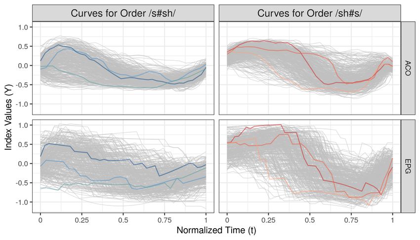
Each functional index varies roughly between +1 and −1 and measures how similar the
13Figure 3: Index curves of the consonant assimilation data set for both ACO and EPG data as a
function of standardized time t (grey curves). For every consonant order, three randomly selected
observations have been highlighted. Every colour corresponds to one multivariate observation,
i.e. one observation consists of two index curves.
articulatory or acoustic pattern is to its reference patterns for the first (+1) and second (−1)
consonant at every observed time point (Cederbaum et al.; 2016). Without assimilation, the
data are thus expected to shift from positive to negative values in a sinus-like form (see Figure
3). The data set contains 707 bivariate functional observations with differently spaced grids of
evaluation points per curve and dimension, with the number of evaluation points ranging from
22 to 59 with a median of 35.
For comparability, we follow the model specification of Cederbaum et al. (2016), who analyse
only the ACO dimension and ignore the second mode EPG. Our specified multivariate model
is similar to (10) with i = 1, ..., 9 the speaker index, j = 1, ..., 16 the word combination in-
dex, h = 1, ..., Hij the repetition index and t ∈ [0, 1] relative time. Note that the nested effect
Cij (t) is replaced by the crossed random effect Cj (t) specific to the word combinations. The
additive predictor µ(xj , t) now contains eight partial effects: the functional intercept plus main
and interaction effects of scalar covariates describing characteristics of the word combination
such as the order of the consonants /s/ and /sh/. The white noise measurement error ijht is
assumed to follow a zero-mean bivariate normal distribution with diagonal covariance matrix
2 2
diag(σACO , σEPG ). The basis and penalty specifications follow the univariate analysis in Ceder-
baum et al. (2016). Given different sampling mechanisms, we also compare the multiFAMM
based on weighted and unweighted scalar products for the MFPCA.
Results
The multivariate analysis supports the findings of Cederbaum et al. (2016) that assimilation
is asymmetric (different mean patterns for /s#sh/ and /sh#s/). Overall, the estimated fixed
effects are similar across dimensions as well as comparable to the univariate analysis. Hence, the
multivariate analysis indicates that previous results for the acoustics are consistently found also
for the articulation. Compared to univariate analyses, our approach reduces the number of FPC
basis functions and thus the number of parameters in the analysis. The multiFAMM can improve
14the model fit and can provide smaller CBs for the ACO dimension compared to the univariate
model in Cederbaum et al. (2016) due to the strong cross-correlation between the dimensions.
We find similar modes of variation for the multivariate and the univariate analysis as well as
across dimensions. In particular, the word combination-specific random effect Cj (t) is dropped
from the model as much of the between-word variation is already explained by the included fixed
effects. The definition of the scalar product has little effect on the estimated fixed effects but
changes the interpretation of the FPCs. Appendix C contains a more in depth description of
this application.
5 Simulations
5.1 Simulation Set-Up
We conduct an extensive simulation study to investigate the performance of the multiFAMM
depending on different model specifications and data settings (over 20 scenarios total), and to
compare it to univariate regression models as proposed by Cederbaum et al. (2016), estimated
on each dimension independently. Given the broad scope of analysed model scenarios, we refer
the interested reader to Appendix D for a detailed report and restrict the presentation here to
the main results.
We mimic our two presented data examples (Section 4) and simulate new data based on
the respective multiFAMM-fit. Each scenario consists of model fits to 500 generated data sets,
where we randomly draw the number and location of the evaluation points, the random scores,
and the measurement errors according to different data settings. The accuracy of the estimated
model components is measured by the root relative mean squared error (rrMSE) based on the
unweighted multivariate norm but otherwise as defined by Cederbaum et al. (2016), see Appendix
D.1. The rrMSE takes on (unbounded) positive values with smaller values indicating a better
fit.
5.2 Simulation Results
Figure 4 compares the rrMSE values over selected modeling scenarios based on the consonant
assimilation data. We generate a benchmark scenario (dark blue), which imitates the original
data without misspecification of any model component. In particular, the number of FPCs is fixed
to avoid truncation effects. Comparing this scenario to the other blue scenarios illustrates the
importance of the number of FPCs in the accuracy of the estimation. Choosing the truncation lag
via the proportion of univariate variance explained (Cut-Off Uni) gives models with roughly the
same number of FPCs (mean B : 2.8, E : 5) as is used for the data generation (B : 3, E : 5). The
cut-off criterion based on the multivariate variance (Cut-Off Mul) results in more parsimonious
models (mean B : 2.15, E : 4) and thus considerably higher rrMSE values. Comparing the
benchmark scenario to more sparsely observed functional data (ceteris paribus) suggests a lower
estimation accuracy for the Sparse Data scenario, especially for the fitted curves yijh (t) and the
curve-specific random effect Eijh (t). The estimation of the mean µ(xij , t), however, is quite
robust against the increased uncertainty of these three scenarios. Only when the random scores
are not centred and decorrelated as in the benchmark scenario do we find an increase in rrMSE
values for the mean (Uncentred Scores). This corresponds to a departure from the modeling
assumptions likely to occur in practice when only few levels of a random effect are available
(here for the subject-specific Bi (t)). The model then has difficulties to separate intercept and
random effects, which does not necessarily translate to a worse overall fit to the data yijh (t) or
to the other fixed effects (cf. Appendix Figure 31).
15Figure 4: rrMSE values of the fitted curves yijh (t), the mean µ(xij , t), and the random effects
Bi (t) and Eijh (t) for different modeling scenarios. Scenarios coloured with blue correspond to
different model specifications in the same data setting.
Our simulation study thus suggests that basing the truncation lags on the proportion of
explained variation on each dimension gives parsimonious and well fitting models. If interest
lies mainly in the estimation of fixed effects, the alternative cut-off criterion based on the total
variation in the data allows even more parsimonious models. Furthermore, the results presented
in Appendix D show that the mean estimation is relatively stable over different model scenarios
including misspecification of the measurement error variance structure or of the multivariate
scalar product, as well as in scenarios with strong heteroscedasticity across dimensions. In our
benchmark scenario, the CBs cover the true effect 89 − 94% of the time but coverage can further
decrease with additional uncertainty e.g. about the number of FPCs. Overall, the covariance
structure such as the leading FPCs can be recovered well, also for a nested random effect such
as in the snooker training application. The comparison to the univariate modeling approach
suggests that the multiFAMM can improve the mean estimation but is especially beneficial for
the prediction of the random effects while reducing the number of parameters to estimate. In
some cases like strong heteroscedasticity, including weights in the multivariate scalar product
might further improve the modeling.
6 Discussion
The proposed multivariate functional regression model is an additive mixed model, which allows
to model flexible covariate effects for sparse or irregular multivariate functional data. It uses FPC
based functional random effects to model complex correlations within and between functions
and dimensions. An important contribution of our approach is estimating the parsimonious
multivariate FPC basis from the data. This allows us to account not only for auto-covariances,
but also for non-trivial cross-covariances over dimensions, which are difficult to adequately model
using alternative approaches such as parametric covariance functions like the Matèrn family
or penalized splines, which imply a parsimonious covariance only within but not necessarily
between functions. As a FAMM-type regression model, a wide range of covariate effect types is
16available, also providing pointwise CBs. Our applications show that the multiFAMMs can give
valuable insight into the multivariate correlation structure of the functions in addition to the
mean structure.
An apparent benefit of multivariate modeling is that it allows to answer research questions
simultaneously relating to different dimensions. In addition, using multivariate FPCs reduces
the number of parameters compared to fitting comparable univariate models while improving
the random effects estimation by incorporating the cross-covariance in the multivariate analysis.
The added computational costs are small: For our multimodal application, the multivariate
approach prolongs the computation time by only five percent (104 vs. 109 minutes on a 64-bit
Linux platform).
We find that the average point-wise coverage of the point-wise CBs can in some cases lie
considerably below the nominal value. There are two main reasons for this: One, the CBs
presented here do not incorporate the uncertainty of the eigenfunction estimation nor of the
smoothing parameter selection. Two, coverage issues can arise in (scalar) mixed models, if effect
functions are estimated as constant when in truth they are not (e.g. Wood; 2017; Greven and
Scheipl; 2016). To resolve these issues, further research on the level of scalar mixed models might
be needed. A large body of research covering CB estimation for functional data (e.g. Goldsmith
et al.; 2013; Choi and Reimherr; 2018; Liebl and Reimherr; 2019) suggests that the construction
of CBs is an interesting and complex problem, also outside of the FAMM framework.
It would be interesting to extend the multiFAMM to more general scenarios of multivariate
functional data such as observations consisting of functions with different dimensional domains,
e.g. functions over time and images as in Happ and Greven (2018). This would require adapting
the estimation of the univariate auto-covariances for spatial arguments t, t0 . Exploiting properties
of dense functional data, such as the block structure of design matrices for functions observed
on a grid, could help to reduce computational cost in this case. Future research could further
generalize the covariance structure of the multiFAMM by allowing for additional covariate effects.
In our snooker training application, for example, a treatment effect of the snooker training might
show itself in the form of reduced intra-player variance (cf. Backenroth et al.; 2018). Ideas
from distributional regression could be incorporated to jointly model the mean trajectories and
covariance structure conditional on covariates.
Acknowledgements
We thank Timon Enghofer, Phil Hoole, and Marianne Pouplier for providing access to their data
and for fruitful discussions. We also thank Lisa Steyer for contributing the data registration
of the snooker training data. Sonja Greven, Almond Stöcker, and Alexander Volkmann were
funded by grant GR 3793/3-1 from the German research foundation (DFG). Fabian Scheipl was
funded by the German Federal Ministry of Education and Research (BMBF) under Grant No.
01IS18036A.
References
Backenroth, D., Goldsmith, J., Harran, M. D., Cortes, J. C., Krakauer, J. W. and Kitago,
T. (2018). Modeling motor learning using heteroscedastic functional principal components
analysis, Journal of the American Statistical Association 113(523): 1003–1015.
Carroll, C., Müller, H.-G. and Kneip, A. (2020). Cross-component registration for multivariate
functional data, with application to growth curves, Biometrics to appear.
17You can also read